| Issue |
A&A
Volume 643, November 2020
|
|
|---|---|---|
| Article Number | A31 | |
| Number of page(s) | 9 | |
| Section | Astrophysical processes | |
| DOI | https://doi.org/10.1051/0004-6361/201937097 | |
| Published online | 27 October 2020 | |
Models of high-frequency quasi-periodic oscillations and black hole spin estimates in Galactic microquasars
1
Research Centre for Computational Physics and Data Processing, Institute of Physics, Silesian University in Opava, Bezručovo nám. 13, 746 01 Opava, Czech Republic
e-mail: This email address is being protected from spambots. You need JavaScript enabled to view it.
2
Research Centre of Theoretical Physics and Astrophysics, Institute of Physics, Silesian University in Opava, Bezručovo nám. 13, 746 01 Opava, Czech Republic
3
Astronomical Institute, Academy of Sciences, Boční II 1401, 14131 Praha 4-Spořilov, Czech Republic
4
Max Planck Institute for Extraterrestrial Physics, Gießenbachstraße 1, 85748 Garching, Germany
5
LESIA, Observatoire de Paris, Université PSL, CNRS, Sorbonne Universités, UPMC Univ. Paris 06, Univ. de Paris, Sorbonne Paris Cité, 5 place Jules Janssen, 92195 Meudon, France
6
Nicolaus Copernicus Astronomical Centre, Polish Academy of Sciences, Bartycka 18, 00-716 Warsaw, Poland
7
Department of Physics, Göteborg University, Sweden
Received:
11
November
2019
Accepted:
26
August
2020
Abstract
We explore the influence of nongeodesic pressure forces present in an accretion disc on the frequencies of its axisymmetric and nonaxisymmetric epicyclic oscillation modes. We discuss its implications for models of high-frequency quasi-periodic oscillations (QPOs), which have been observed in the X-ray flux of accreting black holes (BHs) in the three Galactic microquasars, GRS 1915+105, GRO J1655−40, and XTE J1550−564. We focus on previously considered QPO models that deal with low-azimuthal-number epicyclic modes, |m| ≤ 2, and outline the consequences for the estimations of BH spin, a ∈ [0, 1]. For four out of six examined models, we find only small, rather insignificant changes compared to the geodesic case. For the other two models, on the other hand, there is a significant increase of the estimated upper limit on the spin. Regarding the falsifiability of the QPO models, we find that one particular model from the examined set is incompatible with the data. If the spectral spin estimates for the microquasars that point to a > 0.65 were fully confirmed, two more QPO models would be ruled out. Moreover, if two very different values of the spin, such as a ≈ 0.65 in GRO J1655−40 and a ≈ 1 in GRS 1915+105, were confirmed, all the models except one would remain unsupported by our results. Finally, we discuss the implications for a model that was recently proposed in the context of neutron star (NS) QPOs as a disc-oscillation-based modification of the relativistic precession model. This model provides overall better fits of the NS data and predicts more realistic values of the NS mass compared to the relativistic precession model. We conclude that it also implies a significantly higher upper limit on the microquasar’s BH spin (a ∼ 0.75 vs. a ∼ 0.55).
Key words: X-rays: binaries / black hole physics / accretion, accretion disks
© ESO 2020
1. Introduction
Studying the X-ray spectra and variability provides a powerful tool for putting constraints on properties of compact objects such as mass, M, and spin, a ≡ cJ/(GM2), of a black hole (BH). Among promising methods to measure the BH spin is fitting the X-ray spectral continuum or the relativistically broadened iron Kα lines (McClintock & Remillard 2006; Shafee et al. 2008; Steiner et al. 2009). Various approaches based on X-ray timing, which are complementary to spectral methods, have been gaining popularity as well. One of them is the determination of BH properties using observations of high-frequency quasi-periodic oscillations (HF QPOs)1 and related proposed models.
Detections of elusive HF QPO peaks in Galactic microquasars are frequently reported at rather constant frequencies, which usually appear in ratios of small natural numbers (Abramowicz & Kluźniak 2001; Remillard et al. 2002; McClintock & Remillard 2006). Two peaks often appear that form a 3:2 frequency ratio, R = νU/νL = 3/2, where νU (νL) is the higher (lower) of the two QPO frequencies (see, however, Belloni et al. 2012; Belloni & Altamirano 2013; Varniere & Rodriguez 2018). The evidence for rational frequency ratios has also been discussed in the context of neutron star (NS) QPOs. In the NS sources, clustering of twin-peak QPO detections most frequently arises as a result of weakness of (one or both) QPOs outside the limited range of the QPO frequencies (frequency ratio); see Abramowicz et al. (2003), Belloni et al. (2005, 2007), Török et al. (2008a,b), Barret & Boutelier (2008), Boutelier et al. (2010).
It has been argued that, since the QPO frequencies roughly correspond to timescales of orbital motion in the vicinity of BHs, the phenomenon likely originates in the innermost parts of accretion discs or in their corona. A number of papers have been devoted to the discussion of the determination of M and a that stems from this premise. Different QPO models incorporate different physical concepts in which the QPO excitation radii are located within the most luminous accretion region, usually below r = 20 rG (where rG ≡ GM/c2). Several models, for example, assume that QPOs are produced by a local motion of accreted inhomogeneities, such as blobs or vortices. This subset of QPO models includes the so-called relativistic precession (RP) or the tidal disruption model (Abramowicz et al. 1992; Stella & Vietri 1998, 1999; Čadež et al. 2008; Kostić et al. 2009; Bakala et al. 2014; Karssen et al. 2017; Germanà 2017). Another possibility is to relate the QPOs to a collective motion of the accreted matter, in particular to some accretion disc oscillatory modes that have been explored for both thin and thick discs Kato & Fukue (1980), Okazaki et al. (1987), Nowak & Wagoner (1992), Wagoner (1999), Abramowicz & Kluźniak (2001), Kato (2001), Wagoner et al. (2001), Silbergleit et al. (2001), Wang et al. (2015), Rezzolla et al. (2003), Török et al. (2005), Ingram & Done (2010), Fragile et al. (2016), Stuchlík et al. (2012, 2013, 2020), Ortega-Rodríguez et al. (2020), Maselli et al. (2020). Despite the large efforts made over the past three decades to explain this phenomenon, and a good number of proposed QPO models, until now there has remained no clear consensus on the precise physical mechanism responsible for its occurrence. In several massive extragalactic sources, features that are analogous to QPOs in microquasars (but occur at much lower frequencies) have also been reported and discussed, namely in the context of the properties of their central BH (Goluchová et al. 2019; Gupta et al. 2019).
The RP model proposed two decades ago is often used for the estimation of NS and BH parameters based on the QPOs. Other miscellaneous competing models have been used as well. It is well known, for instance, that the RP model predicts a rather low BH spin for Galactic microquasars, which is in contradiction with some spectral spin estimates. Numerous other estimates based on a large variety of QPO models have been carried out by various authors (the list of references can be found in, e.g., Török et al. 2011; Goluchová et al. 2019). Most of them were made considering a geodesic accretion flow. In more general flows, nongeodesic effects connected to, for example, pressure gradients, magnetic fields, or other forces may have a potentially significant impact on the QPO-based spin predictions.
In this work, we aim to quantify this impact in the particular case of a nongeodesic influence that originates in the pressure forces that are present in the accretion flow modeled by a slightly nonslender pressure-supported perfect fluid torus. We study a specific group of “disc-oscillation” models that involve various combinations of epicyclic modes of accretion disc oscillations. Following our recent work (Šrámková et al. 2015; Török et al. 2016), we primarily focus on comparing two prominent models. Firstly, a model that deals with axisymmetric modes that in the slender torus limit exhibit frequencies equal to the radial and vertical epicyclic frequencies of perturbed geodesic motion. Secondly, a model that in the slender torus limit exhibits the same observable frequencies as the RP model.
The paper is organized as follows. In Sects. 2–4, we shortly recall the physical description of nonslender accretion discs, QPO models, and the applied methodology. In Sect. 5, we focus on comparing BH spin estimates based on the two above-mentioned models. All relevant premises and findings regarding these models are explored here in detail. Section 6 provides a comprehensive extension of the approach introduced in Sect. 5 to several other previously considered QPO models. In Sect. 7, we provide a brief overall quantitative summary, and furthermore we explore the main consequences and state our main concluding remarks.
2. Accretion tori
We consider oscillations of nonslender pressure-supported tori (thick discs) that are made by a perfect polytropic fluid and surround rotating Kerr BHs. Following our previous studies, we assume the specific angular momentum distribution of the flow (defined through the covariant time and azimuthal components of the flow velocity) to be constant within the whole volume of the torus2,
 (1)
(1)
as opposed to the Keplerian distribution,
 (2)
(2)
characteristic for geometrically thin Keplerian flows (thin discs) whose radial structure is mostly determined by a balance between the gravitational and inertial forces.
2.1. Stable configurations of thick relativistic discs
For constant angular momentum tori, Abramowicz et al. (1978; see also Kozlowski et al. 1978) have shown that equilibrium structures of the equipressure and equidensity surfaces coincide with those of the constant effective potential surfaces determined by
 (3)
(3)
Here, gμν denote components of the spacetime metric expressed in the Boyer–Lindquist coordinates. The surface of the torus coincides with one of the equipotential surfaces where the pressure vanishes. The critical points (extrema and saddles) of the effective potential correspond to vanishing pressure gradients and thus to time-like circular geodesics. At these points, the rotation of the flow is Keplerian. The centre of the torus (i.e. the circle at r = rc where the pressure has its maximum) corresponds to a stable time-like circular geodesic located at the local minimum of the effective potential in the equatorial plane.
For angular momenta inside a specific range, there can be another unstable circular geodesic that corresponds to the saddle point of the effective potential and puts a limit on the possible size of the torus located at a given rc. The related critical equipotential has a characteristic “cusp” through which the matter may be accreted onto the central BH without the need for any viscous processes, similarly to the well-known Roche-lobe overflow in binary systems (Kozlowski et al. 1978).
2.2. The inner edge
While the marginally stable circular orbit, rms, is often called the innermost stable circular orbit (ISCO) of a thin accretion disc and forms its inner edge, the inner edge of a thick disc has a different location. Situated between rms and the marginally bound circular orbit, rmb, this location depends on the angular momentum of the disc, ℓc (Abramowicz et al. 1978). For ℓc > ℓK(rmb), the disc is infinite with its inner edge located at rmb, but still well inside the cusp self-crossing equipotential. The ℓc = ℓK(rmb) case corresponds to an infinite torus terminated by the cusp at rmb. For ℓc < ℓK(rmb), the configuration corresponds to a finite, marginally overflowing torus. This torus has its inner edge located closer to BH than rms, but not closer than rmb.
Examples of various tori configurations are illustrated in the left panel of Fig. 1. While the equilibrium configuration of fluid that embodies the cusp equipotential represents a rather simplified stationary analytic model of a non-accreting disc, in accretion, the very existence of the cusp is of general importance. As long as the disc dynamical timescale is significantly shorter than the viscous timescale, which is true for most disc models, the cusp plays a key role in the accretion of matter onto the BH. Fluid elements above the cusp inside the torus stay at more or less the same radius for a large number of dynamical periods, whereas below the cusp accretion is more of a Bondi-like type. The presence of the cusp is indeed often seen in sophisticated numerical simulations of accretion flows (e.g. Qian et al. 2009; Fragile et al. 2007, 2009; Gimeno-Soler & Font 2017; Lančová et al. 2019). This is illustrated in the right panel of Fig. 1.
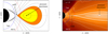 |
Fig. 1. Left: illustration of the topology of equipotential surfaces that determines the spatial distribution of fluid in thick discs (often called Polish doughnuts). The yellow region corresponds to tori of various thicknesses. The orange (along with yellow) region corresponds to a torus with a cusp. The topology allows for many discs with no cusp (β < βcusp) and one disc with a cusp (β = βcusp). The self-crossing equipotential curve corresponds to the marginally overflowing torus with ℓK(rms) < ℓc < ℓK(rmb). The torus has a finite extent and is terminated by a cusp located at its inner edge. The coloured lines corresponding to constant radii denote the marginally stable (ISCO) and marginally bound (rmb) orbit. A more detailed illustration along with rigorous classification of possible equipotential curve topologies can be found in Abramowicz et al. (1978). Right: equipressure contours seen within an up-to-date general relativistic three-dimensional global radiative magnetohydrodynamic simulation. The figure is based on the work of Lančová et al. (2019) who reported a new class of realistic solutions of BH accretion flows – the so-called puffy accretion discs. The setup of the simulation is very general and does not assume any form of initial toroidal structure of the fluid within the inner accretion region. |
2.3. Torus size
To quantify the torus size, Abramowicz et al. (2006) introduced the “thickness” β parameter,
 (4)
(4)
where n is the polytropic index and csc,  , Ωc are the polytropic sound speed, the contravariant time component of the four-velocity, and the angular velocity of the flow defined at the centre of the torus, r = rc. For angular momenta ℓK(rms) < ℓc < ℓK(rmb), this parameter is limited by
 (5)
(5)
whereas, for ℓc ≥ ℓK(rmb), the possible range of β is given by
 (6)
(6)
Here, Wc and Wcusp are the effective potential values corresponding to the centre and cusp equipotential.
In general, the value of β that corresponds to marginally overflowing tori, β = βcusp(a), lies in the range
 (7)
(7)
where βcusp(a) = 0 describes a torus located at the marginally stable circular orbit, rms = rms(a). For the purpose of the present work, it is useful to introduce the “effective” β parameter,
 (8)
(8)
For ℓc ≥ ℓK(rmb), the possible equilibrium configurations correspond to 0 ≤ βeff ≤ 1, while, for ℓK(rms) < ℓc < ℓK(rmb), the allowed range is 0 ≤ βeff ≤ βcusp/β∞. Based on the value of βeff, one may determine whether a given cusp configuration corresponds to a small torus, or to a large torus with β ≈ β∞.
3. Models of quasi-periodic oscillations under consideration
There is a large collection of papers suggesting that QPOs are related to oscillations of accretion tori (Abramowicz & Kluźniak 2001; Rezzolla et al. 2003; Abramowicz et al. 2006; Ingram & Done 2010; Fragile et al. 2016; de Avellar et al. 2018). These studies often assume that oscillations of tori can be responsible for both BH and NS QPOs, the large differences between the two classes of sources being related mostly to a different QPO modulation mechanism (Bursa et al. 2004; Horák 2005; Abramowicz et al. 2006). A subset of these studies focus on the epicyclic modes of torus oscillations. Based on the evidence for the 3:2 QPO frequency ratio, it is often speculated that the QPOs are connected to a non-linear resonant coupling between different pairs of these modes.
In this work, we continue the efforts to study the epicyclic modes of torus oscillations in the context of fitting the observed QPO frequencies. We presume that the two oscillatory modes identified with the observed 3:2 QPOs are excited at the same radius and under the same physical conditions (i.e. the same torus configuration). This assumption is valid not only for the resonance-based concepts but also for a broader class of models. In this sense, our study is relevant to the consideration of the epicyclic oscillation modes in a more general context. In what follows, as well as in our previous studies, we refer to different combinations of epicyclic modes as different QPO models, although they could be in principle viewed as different versions of just one model, which deals with the epicyclic oscillations of thick discs.
Generally speaking, the probability of exciting a given mode with a certain amplitude decreases with increasing azimuthal wave number m. We consider situations characterized by |m| ≤ 2. We further restrict our attention to several models that are based on various physical motivations suggested in preceding studies. In some cases, apart from disc oscillation modes, these models also deal with the Keplerian circular motion. Two of these models have been favoured since they exhibit the potential for resonant coupling (group A). The others represent alternatives of two models previously elaborated and supported within numerous papers in the context of thin discs (group B). All these models except one were used in the work of Török et al. (2011) who calculated BH spin values for a purely geodesic flow in the three Galactic microquasars with HF QPOs – GRS 1915+105, GRO J1655−40, and XTE J1550−564.
3.1. Group A
No fully self-consistent concept of resonant models that would incorporate some of the epicyclic modes has been proposed so far. Despite it being a necessary requirement, the frequency commensurability is not a sufficient condition for the resonance to occur. Other important requirements follow from the symmetry properties of the involved oscillatory modes, such as their parities with respect to the equatorial plane or the azimuthal wavenumber. Out of all oscillatory mode combinations discussed in this work, only the axisymmetric modes seem to fully satisfy these conditions (Horák 2008).
In this context, we examine the “epicyclic” (Ep) model of Abramowicz and Kluźniak, which attributes the HF QPOs to the axisymmetric radial and vertical epicyclic oscillation modes in the accretion disc. Alternatively, in the so-called Kep model, the two QPO frequencies are associated with the axisymmetric radial mode frequency and the Keplerian orbital frequency (see Török et al. 2005, for details). Both models have been extensively studied by Abramowicz & Kluźniak (2001), Abramowicz et al. (2003), Kluźniak et al. (2004), Horák & Karas (2006) and Horák et al. (2009).
3.2. Group B
There are two combinations of modes, which we denote the “RP1” model (Bursa et al. 2005) and the “RP2” model (Török et al. 2010). In the slender torus limit, for a non-rotating BH, these two models predict the same observable frequencies as the RP model. In this limit, for any BH spin, the same observable frequencies as those predicted by the RP model are also predicted by another combination of modes that we denote the RP0 model in what follows. This model deals with the possibility of the observed QPO frequencies being associated to the m = −1 non-axisymmetric radial mode frequency and the Keplerian orbital frequency. We consider the RP0 model in addition to the set of models discussed by Török et al. (2011). The RP0 model is of special importance in the context of the recent findings on NS QPOs presented in the studies of Török et al. (2016, 2018, 2019), which is further discussed in Sect. 7.2.
Finally, we also assume a combination of modes that in the slender torus limit leads to the same observable frequencies as the “warped disc” model proposed by Kato (2001, 2004) in the context of discoseismology (the study of oscillations of thin discs); we refer to this as the WD model.
4. Epicyclic mode frequencies
In Table 1, we list the formulae for the observable QPO frequencies for each of the above models. In the slender torus limit, they are expressed in terms of frequencies of geodesic orbital motion, i.e. the Keplerian orbital frequency, νK, and the radial and vertical epicyclic frequencies, νr and νθ, which, in the Boyer–Lindquist coordinates, t, r, θ, ϕ, may be written as (e.g. Aliev & Galtsov 1981; Silbergleit et al. 2001; Török & Stuchlík 2005)
 (9)
(9)
 (10)
(10)
Frequency relations corresponding to QPO models considered in this work, listed for both the non-geodesic case and the slender torus limit.
where
 (11)
(11)
 (12)
(12)
 (13)
(13)
 (14)
(14)
4.1. Epicyclic mode frequencies in non-slender tori
In non-slender tori, the frequencies of oscillation modes are modified by the pressure forces. As a result, the non-geodesic radial and vertical epicyclic frequencies will differ from those corresponding to the perturbed circular geodesic motion.
The study of oscillation and stability properties of fluid tori was initiated by Papaloizou & Pringle (1984), who explored the global linear stability of Newtonian fluid tori with respect to non-axisymmetric perturbations. Considering small linear perturbations to the torus equilibrium, these latter authors derived a single partial differential equation governing the linear dynamics of oscillations of a Newtonian constant specific angular momentum torus (Papaloizou & Pringle 1984). Later, a general relativistic form of the Papaloizou–Pringle equation was introduced by Abramowicz et al. (2006) and Blaes et al. (2006). In general, this equation cannot be fully solved analytically. Using a perturbation method, Straub & Šrámková (2009) and Fragile et al. (2016) derived fully general relativistic formulae determining the frequencies of axisymmetric and non-axisymmetric radial and vertical epicyclic modes in a slightly non-slender constant specific angular momentum torus within a second-order accuracy in the torus thickness.
Using relations (9)–(14), the calculated frequencies of the radial and vertical epicyclic modes can be written in the following form:
![Mathematical equation: $$ \begin{aligned} \nu _{\mathrm{r} ,\,m}^*&=\left[\sqrt{\alpha _{\rm r}} + m + \beta ^2 C_{\mathrm{r} ,\,m}(r_{\mathrm{c}},a)\right]\nu _{\rm K}\\&=\nu _{\mathrm{r} } + \left[ m + \beta ^2 C_{\mathrm{r} ,\,m}(r_{\mathrm{c}},a)\right]\nu _{\rm K}\nonumber ,\end{aligned} $$](/articles/aa/full_html/2020/11/aa37097-19/aa37097-19-eq26.gif) (15)
(15)
![Mathematical equation: $$ \begin{aligned} \nu _{\theta ,\,m}^*&=\left[\sqrt{\alpha _\theta } + m + \beta ^2 C_{\theta ,\,m}(r_{\mathrm{c}},a)\right]\nu _{\rm K}\\&=\nu _{\theta } + \left[m + \beta ^2 C_{\theta ,\,m}(r_{\mathrm{c}},a)\right]\nu _{\rm K}\nonumber . \end{aligned} $$](/articles/aa/full_html/2020/11/aa37097-19/aa37097-19-eq27.gif) (16)
(16)
Here, m is the azimuthal wavenumber, and Cr, m(rc, a) and Cθ, m(rc, a) denote the negative second-order pressure corrections evaluated at the centre of the torus, r = rc. Since Cr, m and Cθ, m are given by fairly long expressions, we provide their explicit form within a Wolfram Mathematica notebook3.
4.2. The approximative formulae applicability
It is necessary to determine the range of the β parameter relevant for our study. Formulae (15) and (16) should provide reasonable results for tori of a moderate thickness, but they are not fully applicable for tori of substantial widths. To specify this statement quantitatively, a particular physical situation needs to be taken into account. It is useful to express the torus thickness in terms of βeff. One could expect βeff ∼ 0.3 to likely yield a solid approximation of a real situation, while considering βeff ∼ 0.7 could lead to incorrect results. In what follows, we use βeff = 0.3 and βeff = 0.7 as the referential values.
5. BH spin estimation: Ep and RP0 models
In order to obtain the constraints on M and a, we make a comparison between the expected and the observed QPO frequencies. Following Török et al. (2011), we compare the predicted frequencies to the observed frequencies in the specific case of the 3:2 frequency ratio (see Sect. 7 for a further discussion). The predictions of geodesic QPO models are illustrated in Fig. 2. Šrámková et al. (2015) applied the results of Straub & Šrámková (2009) to study the particular case of the Ep model. Following the previous studies on BH spin estimations (Kluźniak & Abramowicz 2001; Török et al. 2005, 2011), they used the QPO independent mass estimates. The main conclusion of their work is that the effect of the pressure forces on the predicted QPO frequencies is very small when a < 0.9. The influence becomes significant only for rapidly rotating BHs (a > 0.9).
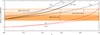 |
Fig. 2. M(a) curves implied by the geodesic QPO models. The predictions of the RP0 model fully coincide with those of the RP model. The orange horizontal rectangles covering the full range of a indicate the commonly accepted limits on the BH mass in each microquasar. |
Fragile et al. (2016) derived corrections to formulae for non-geodesic epicyclic frequencies assuming the exact form of the relativistic Papaloizou–Pringle equation as oppose to the approximative form considered by Blaes et al. (2006, 2007) and Straub & Šrámková (2009). Here, we use their formulae to revise the calculations of Šrámková et al. (2015) carried out for the Ep model and, furthermore, to extend this approach to another QPO model: the RP0 model.
5.1. Behaviour of frequencies of quasi-periodic oscillations
Although we mostly focus on the 3:2 frequency ratio, other frequency ratios are explored as well. Figure 3 shows the results of such an investigation for the Schwarzschild spacetime and tori whose thickness ranges from an infinitely slender torus to a torus with its outer edge extending to infinity. The QPO frequency ratio in Fig. 3 is not fixed and takes values of up to R = 10.
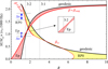 |
Fig. 3. Upper QPO frequency predicted by the Ep and RP0 model plotted for a = 0 and tori whose thickness ranges from an infinitely slender torus (β = 0, black line) through a torus with a cusp (β = βcusp, red line) to a torus whose outer edge extends to infinity (βeff = 1, dotted red line). The blue arrows indicate the spread of the resonant frequency implied by the allowed spread of β for each model and the 3 : 2 QPO frequency ratio. |
The enlarged area in Fig. 3 illustrates the QPO frequency behaviour relevant for the Ep model close to R = 3 : 2. It is apparent that for ratios from this area, the extremal value of the QPO frequency does not always correspond to a torus with a cusp. Such a phenomenon was discussed in more detail in our previous paper (Šrámková et al. 2015).
The position of the orbit that gives the 3:2 QPO frequency ratio within the Ep model changes in a non-trivial way as the torus size increases. As a consequence, the relation between β and the QPO frequency is not always a function (Blaes et al. 2006; Šrámková et al. 2015); see the loops on the Ep model curves illustrated in Fig. 4. Nevertheless, for a = 0, these frequencies only display a small variation across the whole range of allowed torus thicknesses. The low sensitivity of the predicted QPO frequency to torus thickness persists up to a ∼ 0.9.
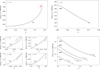 |
Fig. 4. Comparison between the upper QPO frequencies predicted by the Ep and RP0 models. Left: examples of the non-trivial topology of νU(β) curves predicted by the Ep model. Except for the a = 0 case, we do not display the whole effective range of β ∈ [0, βcusp]; the overall increase of νU is rather small for any a ≲ 0.9. Right: monotonic behaviour of νU(β) functions predicted by the RP0 model. The values of a are the same as in the left panel. In both panels, the red dots correspond to β = βcusp. The empty red circle denotes β = β∞. |
For the RP0 model and the 3:2 frequency ratio, the predicted QPO frequency is a monotonic function of β. This is illustrated in Fig. 4, which shows a comparison between the Ep and RP0 models. We note that, for a ∈ [0, 0.9], the RP0 model is associated with a much higher quantitative impact of the torus thickness on the QPO frequency.
5.2. The main implications for BH spin
Figure 5 shows a comparison between the overall behaviour of the QPO frequencies implied by the Ep and RP0 models as it changes with increasing BH spin and torus thickness. Different curves in the figure indicate the referential values of the relative torus thickness, βeff ∈ 0, 0.3, 0.7, 1. There is only a small spread of the resonant frequency predicted by the Ep model for all but very high spins (a ≳ 0.9). The lower limit on the spin given by this model, a ≈ 0.69 for βeff = 0, reaches the value of a ≈ 0.62 for the maximal allowed torus thickness. The impact of the non-geodesic effects is clearly more important within the RP0 model. For a geodesic limit of this model (which corresponds to the RP model), the maximal value of the spin is about a ∼ 0.55. Regarding larger tori, it can grow up to a ∼ 0.75 for tori with a cusp, or even to a ∼ 0.83 when tori with no cusp are assumed. A detailed quantification of the impact for each microquasar is presented in Table 2.
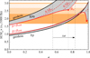 |
Fig. 5. M(a) relation implied by the RP0 and Ep models. The thick black curves correspond to the geodesic case, i.e. these are the same curves as those shown in Fig. 2. The grey shaded region indicates the case when β > 0. The thick red curves correspond to β = βcusp and the dotted red curve to β = β∞. The dashed red lines correspond to βeff = β/β∞ = 0.7 and βeff = β/β∞ = 0.3. The black arrow labelled Δa indicates the shift of the upper limit on the spin of microquasars implied by the RP0 model considering the non-geodesic flow (from a ∼ 0.55 to a ∼ 0.83). |
Intervals of spin implied for the three microquasars by the considered QPO models for the geodesic (a) and non-geodesic (a*) cases.
6. Estimation of BH spin: other models
We plot the spread of the upper QPO frequency implied by the Kep, RP1, RP2, and WD models for a = 0 in the left panel of Fig. 6. The Ep model predictions are presented as well for the sake of comparison. In analogy to Fig. 3, the QPO frequency ratio is not fixed and takes values of up to R = 10. For the 3:2 frequency ratio, the spread of the QPO frequency is rather large within the Kep, RP1, and WD models (contrary to the Ep and RP2 models). We find that similar behaviour of the QPO model frequencies also arises for rotating BHs.
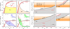 |
Fig. 6. Left: same as in Fig. 3, but for the Kep, RP1, RP2, and WD models. Right: same as in Fig. 5, but for the Kep, RP1, RP2, and WD models. We note that for the RP2 and WD models, we have β ≪ 0.3β∞. |
The right panel of Fig. 6 illustrates the impact of the above-described QPO frequency behaviour on the estimation of BH spin. The QPO frequencies in the limit of β = 0 are increasing monotonic functions of a. The pressure corrections to these frequencies are negative for the Kep and RP1 models, while they are positive for the WD and RP2 models. Out of these four models, only for the RP1 model is there a significant change of the estimated overall upper limit on the spin.
For the Kep model, there is a large spread of the predicted QPO frequency, but the scaled frequency M × νU(a) is clearly lower than the observationally constrained values for any a ≲ 0.79. For this reason, the overall limit on the spin remains unchanged. Within the RP1 model, the geodesic curve enters most of the observationally constrained region (a ∈ [0, 0.78]), and the influence of a non-zero torus thickness raises the upper limit to a = 1. Within the WD and RP2 models, the scaled frequencies M × νU(a) are higher than the observationally constrained values for any a ≳ 0.44. The estimated overall upper limit therefore remains unaltered for both these models.
7. Discussion and conclusions
Table 2 indicates how the limit on the spin changes for different models in each microquasar. In all three microquasars, the main conclusions remain mostly unaltered compared to the geodesic case for four out of the six examined models. In particular, there is a small change of the lower limit on the spin in all the three sources in the Ep model case. For the Kep, WD, and RP2 models, the spin estimates for GRS 1915+105 remain fully unaltered, while for the other two sources, there is only a certain decrease of the lower limit on the inferred spin. On the other hand, within the RP0 and RP1 models, the estimated upper limit on the BH spin shows a significant increase.
7.1. The main implications
Regarding the falsifiability of the QPO models, we conclude that much like in the geodesic case the Kep model is fully incompatible with the GRO J1655−40 and XTE 1550−564 data. Provided that the mechanism responsible for the QPO phenomenon is the same in all three microquasars, this model would be ruled out. Although there is currently no final agreement on the spectral spin estimates, the overall sample of the iron line- and continuum-based studies suggests that at least one of the microquasars should exceed the value of a = 0.65 (McClintock et al. 2006, 2014; Middleton et al. 2006; Blum et al. 2009; Miller & Miller 2015). If this were confirmed, our study would additionally rule out the WD and RP2 models. Moreover, if two very different values of the spin, such as a ≈ 0.65 in GRO J1655−40 and a ≈ 1 in GRS 1915+105, were confirmed, all the models except the RP1 model would remain unsupported by our results.
7.2. Favoured models
As briefly mentioned in Sects. 1–3, two of the models considered in this work are of special importance. The first is the Ep model, which is prominent within the class of the resonance models proposed by Abramowicz & Kluźniak (2001) and Török et al. (2005). This model, which involves the axisymmetric modes, is by far the most developed resonance model of QPOs. Using the solution of the improved relativistic Papaloizou–Pringle equation, we confirm the previous result of Šrámková et al. (2015), which indicates low sensitivity of the resonant frequency to the torus thickness, and the requirement of a high BH spin. The second is the RP0 model, which provides outstanding results regarding the overall context of matching the BH and NS HF QPOs.
In the slender torus limit, the RP0 model predicts the same QPO frequencies as the RP model. For the marginally overflowing torus (β = βcusp), it merges with a model recently discussed by Török et al. (2016) in the context of NS QPOs (in next the CT model). The CT model has been suggested as an alternative to the RP model that deals with torus oscillations. It is based on the expectation that cusp configurations are likely to appear in real accretion flows, in which case the actual overall accretion rate through the inner edge of the disc can be strongly modulated by the disc oscillations (Paczynski & Abramowicz 1982; Abramowicz et al. 2006). This model provides generally better fits of the NS data than the RP model. It also predicts a lower NS mass than the RP model, which in some cases implies an overly high mass estimate (Török et al. 2018, 2019).
The spin predicted by the CT model is given by the upper solid red curve in Fig. 5. (The RP0 model and β = βcusp). We conclude that the upper limit on the spin implied by this model is significantly higher than in the RP model case, namely a ∼ 0.75 versus a ∼ 0.55. This is presumably in better agreement with the spectral spin estimates.
7.3. Caveats
One should be aware of the limitations associated with the adopted perturbative approach. The results of our calculations that stem from the consideration of βeff ≳ 0.7 should be confronted with exact numerical treatment of the Papaloizou–Pringle equation4. A similar reservation applies to the consideration of a ≫ 0.9, because for high spins the epicyclic mode frequencies are very sensitive to even small changes in torus thickness.
It is not fully clear to what degree our assumptions match the real situation. We compare the observed 3:2 QPO frequencies with frequencies of the oscillation modes calculated for one particular torus configuration. There are not many observations of HF QPOs available for BH binaries, and even fewer of those that are available display the two peaks simultaneously. The integration time required for the QPO identification is a few orders of magnitude longer than the characteristic QPO period. Furthermore, there are observations suggesting that the BH HF QPO frequencies may vary in time and form continuous correlations similar to those observed in NSs that reach into (but are not necessarily constrained to) the 3:2 frequency ratio range (Belloni et al. 2012; Belloni & Altamirano 2013; Motta et al. 2014; Varniere & Rodriguez 2018). Despite these uncertainties, our assumptions are sufficient for the presented simplified analysis, which provides a brief comparison of BH spin estimates associated to models that deal with different combinations of disc oscillation epicyclic modes.
For the sake of simplicity, we often use the shorter term “QPOs” instead of “HF QPOs” throughout the paper.
We adopt the metric signature in the (−,+,+,+) form.
The relation between β and βeff depends on the specific torus configuration underlying a given QPO model. For all tori configurations considered in this paper, we have β = 0.3β∞ ≈ 0.2 and β = 0.7β∞ ∈ [0.4, 0.6] ≈ 0.5.
Acknowledgments
We acknowledge the Czech Science Foundation (GAČR) grant No. 17-16287S. We also wish to thank the INTER-EXCELLENCE project No. LTI17018 that supports the collaboration between the Silesian University in Opava and the Astronomical Institute in Prague. Furthermore, we acknowledge two internal grants of the Silesian University, SGS/12,13/2019. Last but not least, we would like to express our thanks to the referee whose valuable comments and suggestions have greatly helped to improve the paper.
References
- Abramowicz, M. A., & Kluźniak, W. 2001, A&A, 374, L19 [NASA ADS] [CrossRef] [EDP Sciences] [Google Scholar]
- Abramowicz, M., Jaroszynski, M., & Sikora, M. 1978, A&A, 63, 221 [NASA ADS] [Google Scholar]
- Abramowicz, M. A., Lanza, A., Spiegel, E. A., & Szuszkiewicz, E. 1992, Nature, 356, 41 [NASA ADS] [CrossRef] [Google Scholar]
- Abramowicz, M. A., Karas, V., Kluźniak, W., Lee, W. H., & Rebusco, P. 2003, PASJ, 55, 467 [NASA ADS] [CrossRef] [Google Scholar]
- Abramowicz, M. A., Blaes, O. M., Horák, J., Kluźniak, W., & Rebusco, P. 2006, Classical Quantum Gravity, 23, 1689 [NASA ADS] [CrossRef] [Google Scholar]
- Aliev, A. N., & Galtsov, D. V. 1981, Gen. Relativ. Gravit., 13, 899 [NASA ADS] [CrossRef] [Google Scholar]
- Bakala, P., Török, G., Karas, V., et al. 2014, MNRAS, 439, 1933 [NASA ADS] [CrossRef] [Google Scholar]
- Barret, D., & Boutelier, M. 2008, New Astron. Rev., 51, 835 [NASA ADS] [CrossRef] [Google Scholar]
- Belloni, T. M., & Altamirano, D. 2013, MNRAS, 432, 10 [NASA ADS] [CrossRef] [Google Scholar]
- Belloni, T., Méndez, M., & Homan, J. 2005, A&A, 437, 209 [NASA ADS] [CrossRef] [EDP Sciences] [Google Scholar]
- Belloni, T., Méndez, M., & Homan, J. 2007, MNRAS, 376, 1133 [NASA ADS] [CrossRef] [Google Scholar]
- Belloni, T. M., Sanna, A., & Méndez, M. 2012, MNRAS, 426, 1701 [NASA ADS] [CrossRef] [Google Scholar]
- Blaes, O. M., Arras, P., & Fragile, P. C. 2006, MNRAS, 369, 1235 [NASA ADS] [CrossRef] [Google Scholar]
- Blaes, O. M., Šrámková, E., Abramowicz, M. A., Kluźniak, W., & Torkelsson, U. 2007, ApJ, 665, 642 [NASA ADS] [CrossRef] [Google Scholar]
- Blum, J. L., Miller, J. M., Fabian, A. C., et al. 2009, ApJ, 706, 60 [NASA ADS] [CrossRef] [Google Scholar]
- Boutelier, M., Barret, D., Lin, Y., & Török, G. 2010, MNRAS, 401, 1290 [NASA ADS] [CrossRef] [Google Scholar]
- Bursa, M. 2005, in RAGtime 6/7: Workshops on Black Holes and Neutron Stars, eds. S. Hledík, & Z. Stuchlík, 39 [Google Scholar]
- Bursa, M., Abramowicz, M. A., Karas, V., & Kluźniak, W. 2004, ApJ, 617, L45 [NASA ADS] [CrossRef] [Google Scholar]
- Čadež, A., Calvani, M., & Kostić, U. 2008, A&A, 487, 527 [NASA ADS] [CrossRef] [EDP Sciences] [Google Scholar]
- de Avellar, M. G. B., Porth, O., Younsi, Z., & Rezzolla, L. 2018, MNRAS, 474, 3967 [NASA ADS] [CrossRef] [Google Scholar]
- Fragile, P. C., Blaes, O. M., Anninos, P., & Salmonson, J. D. 2007, ApJ, 668, 417 [NASA ADS] [CrossRef] [Google Scholar]
- Fragile, P. C., Lindner, C. C., Anninos, P., & Salmonson, J. D. 2009, ApJ, 691, 482 [NASA ADS] [CrossRef] [Google Scholar]
- Fragile, P. C., Straub, O., & Blaes, O. 2016, MNRAS, 461, 1356 [NASA ADS] [CrossRef] [Google Scholar]
- Germanà, C. 2017, Phys. Rev. D, 96, 103015 [NASA ADS] [CrossRef] [Google Scholar]
- Gimeno-Soler, S., & Font, J. A. 2017, A&A, 607, A68 [NASA ADS] [CrossRef] [EDP Sciences] [Google Scholar]
- Goluchová, K., Török, G., Šrámková, E., et al. 2019, A&A, 622, L8 [CrossRef] [EDP Sciences] [Google Scholar]
- Gupta, A. C., Tripathi, A., Wiita, P. J., et al. 2019, MNRAS, 484, 5785 [NASA ADS] [Google Scholar]
- Horák, J. 2005, Astron. Nachr., 326, 845 [NASA ADS] [CrossRef] [Google Scholar]
- Horák, J. 2008, A&A, 486, 1 [NASA ADS] [CrossRef] [EDP Sciences] [Google Scholar]
- Horák, J., & Karas, V. 2006, A&A, 451, 377 [NASA ADS] [CrossRef] [EDP Sciences] [Google Scholar]
- Horák, J., Abramowicz, M. A., Kluźniak, W., Rebusco, P., & Török, G. 2009, A&A, 499, 535 [NASA ADS] [CrossRef] [EDP Sciences] [Google Scholar]
- Ingram, A., & Done, C. 2010, MNRAS, 405, 2447 [NASA ADS] [Google Scholar]
- Karssen, G. D., Bursa, M., Eckart, A., et al. 2017, MNRAS, 472, 4422 [NASA ADS] [CrossRef] [Google Scholar]
- Kato, S. 2001, PASJ, 53, 1 [NASA ADS] [CrossRef] [Google Scholar]
- Kato, S. 2004, PASJ, 56, 905 [NASA ADS] [Google Scholar]
- Kato, S., & Fukue, J. 1980, ApJ, 32, 377 [Google Scholar]
- Kluźniak, W., & Abramowicz, M. A. 2001, Acta Phys. Polonica B, 32, 3605 [Google Scholar]
- Kluźniak, W., Abramowicz, M. A., Kato, S., Lee, W. H., & Stergioulas, N. 2004, AJ, 603, L89 [NASA ADS] [CrossRef] [Google Scholar]
- Kostić, U., Čadež, A., Calvani, M., & Gomboc, A. 2009, A&A, 496, 307 [NASA ADS] [CrossRef] [EDP Sciences] [Google Scholar]
- Kozlowski, M., Jaroszynski, M., & Abramowicz, M. A. 1978, A&A, 63, 209 [Google Scholar]
- Lančová, D., Abarca, D., Kluźniak, W., et al. 2019, ApJ, 884, L37 [CrossRef] [Google Scholar]
- Maselli, A., Pappas, G., Pani, P., et al. 2020, ApJ, 899, 139 [CrossRef] [Google Scholar]
- McClintock, J. E., & Remillard, R. A. 2006, Black Hole Binaries (Cambridge: Cambridge University Press), 157 [Google Scholar]
- McClintock, J. E., Shafee, R., Narayan, R., et al. 2006, ApJ, 652, 518 [NASA ADS] [CrossRef] [Google Scholar]
- McClintock, J. E., Narayan, R., & Steiner, J. F. 2014, Space Sci. Rev., 183, 295 [NASA ADS] [CrossRef] [Google Scholar]
- Middleton, M., Done, C., Gierliński, M., & Davis, S. W. 2006, MNRAS, 373, 1004 [NASA ADS] [CrossRef] [Google Scholar]
- Miller, M. C., & Miller, J. M. 2015, Phys. Rep., 548, 1 [NASA ADS] [CrossRef] [MathSciNet] [Google Scholar]
- Motta, S. E., Belloni, T. M., Stella, L., Muñoz-Darias, T., & Fender, R. 2014, MNRAS, 437, 2554 [NASA ADS] [CrossRef] [Google Scholar]
- Nowak, M. A., & Wagoner, R. V. 1992, ApJ, 393, 697 [NASA ADS] [CrossRef] [Google Scholar]
- Okazaki, A. T., Kato, S., & Fukue, J. 1987, PASJ, 39, 457 [Google Scholar]
- Ortega-Rodríguez, M., Solís-Sánchez, H., Álvarez-García, L., & Dodero-Rojas, E. 2020, MNRAS, 492, 1755 [CrossRef] [Google Scholar]
- Paczynski, B., & Abramowicz, M. A. 1982, ApJ, 253, 897 [NASA ADS] [CrossRef] [Google Scholar]
- Papaloizou, J. C. B., & Pringle, J. E. 1984, MNRAS, 208, 721 [NASA ADS] [CrossRef] [Google Scholar]
- Qian, L., Abramowicz, M. A., Fragile, P. C., et al. 2009, A&A, 498, 471 [NASA ADS] [CrossRef] [EDP Sciences] [Google Scholar]
- Remillard, R. A., Muno, M. P., McClintock, J. E., & Orosz, J. A. 2002, ApJ, 580, 1030 [NASA ADS] [CrossRef] [Google Scholar]
- Rezzolla, L., Yoshida, S., & Zanotti, O. 2003, MNRAS, 344, 978 [NASA ADS] [CrossRef] [Google Scholar]
- Shafee, R., McKinney, J. C., Narayan, R., et al. 2008, ApJ, 687, L25 [NASA ADS] [CrossRef] [Google Scholar]
- Silbergleit, A. S., Wagoner, R. V., & Ortega-Rodríguez, M. 2001, ApJ, 548, 335 [NASA ADS] [CrossRef] [Google Scholar]
- Šrámková, E., Török, G., Kotrlová, A., et al. 2015, A&A, 578, A90 [CrossRef] [EDP Sciences] [Google Scholar]
- Steiner, J. F., McClintock, J. E., Remillard, R. A., Narayan, R., & Gou, L. 2009, ApJ, 701, L83 [NASA ADS] [CrossRef] [Google Scholar]
- Stella, L., & Vietri, M. 1998, ApJ, 492, L59 [NASA ADS] [CrossRef] [Google Scholar]
- Stella, L., & Vietri, M. 1999, Phys. Rev. Lett., 82, 17 [NASA ADS] [CrossRef] [Google Scholar]
- Straub, O., & Šrámková, E. 2009, Classical Quantum Gravity, 26, 055011 [NASA ADS] [CrossRef] [Google Scholar]
- Stuchlík, Z., Kotrlová, A., & Török, G. 2012, Acta Astron., 62, 389 [NASA ADS] [Google Scholar]
- Stuchlík, Z., Kotrlová, A., & Török, G. 2013, A&A, 552, A10 [NASA ADS] [CrossRef] [EDP Sciences] [Google Scholar]
- Stuchlík, Z., Kološ, M., Kovář, J., Slaný, P., & Tursunov, A. 2020, Universe, 6, 26 [CrossRef] [Google Scholar]
- Török, G., & Stuchlík, Z. 2005, A&A, 437, 775 [NASA ADS] [CrossRef] [EDP Sciences] [Google Scholar]
- Török, G., Abramowicz, M. A., Kluźniak, W., & Stuchlík, Z. 2005, A&A, 436, 1 [NASA ADS] [CrossRef] [EDP Sciences] [Google Scholar]
- Török, G., Abramowicz, M. A., Bakala, P., et al. 2008a, Acta Astron., 58, 15 [NASA ADS] [Google Scholar]
- Török, G., Bakala, P., Stuchlik, Z., & Čech, P. 2008b, Acta Astron., 58, 1 [NASA ADS] [Google Scholar]
- Török, G., Bakala, P., Šrámková, E., Stuchlík, Z., & Urbanec, M. 2010, ApJ, 714, 748 [NASA ADS] [CrossRef] [Google Scholar]
- Török, G., Kotrlová, A., Šrámková, E., & Stuchlík, Z. 2011, A&A, 531, A59 [NASA ADS] [CrossRef] [EDP Sciences] [Google Scholar]
- Török, G., Goluchová, K., Horák, J., et al. 2016, MNRAS, 457, L19 [NASA ADS] [CrossRef] [Google Scholar]
- Török, G., Goluchová, K., Šrámková, E., et al. 2018, MNRAS, 473, L136 [CrossRef] [Google Scholar]
- Török, G., Goluchová, K., Šrámková, E., Urbanec, M., & Straub, O. 2019, MNRAS, 488, 3896 [CrossRef] [Google Scholar]
- Varniere, P., & Rodriguez, J. 2018, ApJ, 865, 113 [NASA ADS] [CrossRef] [Google Scholar]
- Wagoner, R. V. 1999, Phys. Rep., 311, 259 [NASA ADS] [CrossRef] [Google Scholar]
- Wagoner, R. V., Silbergleit, A. S., & Ortega-Rodríguez, M. 2001, AJ, 559, L25 [NASA ADS] [CrossRef] [Google Scholar]
- Wang, D. H., Chen, L., Zhang, C. M., et al. 2015, MNRAS, 454, 1231 [NASA ADS] [CrossRef] [Google Scholar]
All Tables
Frequency relations corresponding to QPO models considered in this work, listed for both the non-geodesic case and the slender torus limit.
Intervals of spin implied for the three microquasars by the considered QPO models for the geodesic (a) and non-geodesic (a*) cases.
All Figures
|
Fig. 1. Left: illustration of the topology of equipotential surfaces that determines the spatial distribution of fluid in thick discs (often called Polish doughnuts). The yellow region corresponds to tori of various thicknesses. The orange (along with yellow) region corresponds to a torus with a cusp. The topology allows for many discs with no cusp (β < βcusp) and one disc with a cusp (β = βcusp). The self-crossing equipotential curve corresponds to the marginally overflowing torus with ℓK(rms) < ℓc < ℓK(rmb). The torus has a finite extent and is terminated by a cusp located at its inner edge. The coloured lines corresponding to constant radii denote the marginally stable (ISCO) and marginally bound (rmb) orbit. A more detailed illustration along with rigorous classification of possible equipotential curve topologies can be found in Abramowicz et al. (1978). Right: equipressure contours seen within an up-to-date general relativistic three-dimensional global radiative magnetohydrodynamic simulation. The figure is based on the work of Lančová et al. (2019) who reported a new class of realistic solutions of BH accretion flows – the so-called puffy accretion discs. The setup of the simulation is very general and does not assume any form of initial toroidal structure of the fluid within the inner accretion region. |
| In the text | |
|
Fig. 2. M(a) curves implied by the geodesic QPO models. The predictions of the RP0 model fully coincide with those of the RP model. The orange horizontal rectangles covering the full range of a indicate the commonly accepted limits on the BH mass in each microquasar. |
| In the text | |
|
Fig. 3. Upper QPO frequency predicted by the Ep and RP0 model plotted for a = 0 and tori whose thickness ranges from an infinitely slender torus (β = 0, black line) through a torus with a cusp (β = βcusp, red line) to a torus whose outer edge extends to infinity (βeff = 1, dotted red line). The blue arrows indicate the spread of the resonant frequency implied by the allowed spread of β for each model and the 3 : 2 QPO frequency ratio. |
| In the text | |
|
Fig. 4. Comparison between the upper QPO frequencies predicted by the Ep and RP0 models. Left: examples of the non-trivial topology of νU(β) curves predicted by the Ep model. Except for the a = 0 case, we do not display the whole effective range of β ∈ [0, βcusp]; the overall increase of νU is rather small for any a ≲ 0.9. Right: monotonic behaviour of νU(β) functions predicted by the RP0 model. The values of a are the same as in the left panel. In both panels, the red dots correspond to β = βcusp. The empty red circle denotes β = β∞. |
| In the text | |
|
Fig. 5. M(a) relation implied by the RP0 and Ep models. The thick black curves correspond to the geodesic case, i.e. these are the same curves as those shown in Fig. 2. The grey shaded region indicates the case when β > 0. The thick red curves correspond to β = βcusp and the dotted red curve to β = β∞. The dashed red lines correspond to βeff = β/β∞ = 0.7 and βeff = β/β∞ = 0.3. The black arrow labelled Δa indicates the shift of the upper limit on the spin of microquasars implied by the RP0 model considering the non-geodesic flow (from a ∼ 0.55 to a ∼ 0.83). |
| In the text | |
|
Fig. 6. Left: same as in Fig. 3, but for the Kep, RP1, RP2, and WD models. Right: same as in Fig. 5, but for the Kep, RP1, RP2, and WD models. We note that for the RP2 and WD models, we have β ≪ 0.3β∞. |
| In the text | |
Current usage metrics show cumulative count of Article Views (full-text article views including HTML views, PDF and ePub downloads, according to the available data) and Abstracts Views on Vision4Press platform.
Data correspond to usage on the plateform after 2015. The current usage metrics is available 48-96 hours after online publication and is updated daily on week days.
Initial download of the metrics may take a while.