© The Authors 2024

1. Introduction

Accretion discs are responsible for the strong observable radiation emitted by systems of accreting black holes (BHs) or neutron stars (NSs). The analysis of their spectral and timing properties provides an excellent opportunity to explore strong gravity (Frank et al. 2002; Kato et al. 2008) and the super-dense matter equation of state (EoS; Lattimer & Prakash 2007). Here, we are especially motivated by several specific challenges arising in contemporary astrophysical research in the field of X-ray variability.

Throughout the history of X-ray timing observations of low-mass X-ray binaries (LMXBs) of both BH and NS types, numerous intriguing features have been revealed. The most rapid X-ray variability observed in these sources occurs at frequencies of up to a few hundred hertz, with the highest values exceeding 1.2 kHz (Barret et al. 2006; van der Klis 2006). Even though the rapid variability was discovered almost half a century ago, the origin of these so-called high-frequency (HF) quasi-periodic oscillations (QPOs), along with the correlated low-frequency (LF) QPOs, has never been sufficiently explained. Over the years, various models of QPOs have been proposed in an attempt to comprehend the nature of the phenomena (see e.g. Alpar & Shaham 1985; Lamb et al. 1985; Miller et al. 1998; Psaltis et al. 1999; Stella et al. 1999; Abramowicz & Kluźniak 2001; Kato 2001; Kluźniak & Abramowicz 2001a; Wagoner et al. 2001; Titarchuk & Wood 2002; Abramowicz et al. 2003a; Rezzolla et al. 2003a; Kluźniak et al. 2004; Zhang 2004; Bursa 2005; Pétri 2005; Čadež et al. 2008; Wang et al. 2008; Mukhopadhyay 2009; Bachetti et al. 2010; Dönmez et al. 2011; Stuchlík & Kološ 2014; Huang et al. 2016; Le et al. 2016; Germanà 2017; Stuchlík et al. 2020; Wang & Zhang 2020; Smith et al. 2021; Török et al. 2022, and references therein). Most hypotheses link the QPO phenomenon to the orbital motion because the observed QPO frequencies are of the same order as those associated with the orbital motion in the innermost region of accretion discs.

Numerous studies have focused on the possible relation between QPOs and the oscillatory motion of stationary pressure-supported fluid configurations (accretion tori) formed near the central compact object (e.g. Kluźniak & Abramowicz 2001b; Kluźniak et al. 2004; Abramowicz et al. 2003a,b; Rezzolla et al. 2003a,b; Bursa 2005; Török et al. 2005, 2016; Dönmez et al. 2011; de Avellar et al. 2018; Faraji & Trova 2023). In this context, Straub & Šrámková (2009) and Fragile et al. (2016) examined oscillation modes of fluid tori in the Kerr geometry, which describes the space-time around a rotating BH. In their investigation, they evaluated the frequencies of these modes in addition to other calculations. Following their approach, we considered slowly rotating NSs for which the surrounding space-time can be represented by the Hartle-Thorne geometry (Hartle 1967; Hartle & Thorne 1968). This space-time geometry was used in Matuszková et al. (2024, hereafter Paper I), where we provide, for the first time, a comprehensive analytical description of accretion tori around rotating NSs.

In this paper, we focus on the epicyclic oscillation modes and their frequencies, especially on the axisymmetric and first-order non-axisymmetric modes. The first pair of modes corresponds to a simple radial and vertical motion of the torus. In the limit of a slender (zero-thickness) torus, the frequencies of these modes match the radial and vertical epicyclic frequencies of the geodesic motion of a test particle.

Similarly, the second pair of modes (which can be referred to as the precession modes) corresponds to the non-axisymmetric radial and vertical motion of the torus. Moreover, in the limit of a slender torus, the frequencies of these modes match the geodesic periastron and the Lense-Thirring precession frequencies, respectively.

Our paper is organised as follows. In Sect. 2 we briefly recall the properties of accretion tori around rotating NSs studied in Paper I. The derivation of the formulae that determine the oscillation modes of these tori is the primary subject of Sects. 3 and 4. In Sect. 5 special attention is given to investigating the behaviour of the axisymmetric and precession mode frequencies. A complete set of formulae for calculating the frequencies of the epicyclic modes under consideration is provided within a Wolfram Mathematica notebook and additional C++ and PYTHON libraries. In Sect. 6, we analyse the behaviour of these frequencies, with a focus on the astrophysically relevant range of NS parameters. We also provide simplified versions of the formulae for the frequencies of axisymmetric radial and vertical oscillations and the frequencies of the two precession modes in Sect. 7. Finally, in Sect. 8 we demonstrate the applications of our formulae to various astrophysically relevant examples, provide a short summary, and state our main concluding remarks.

2. Accretion tori around rotating neutron stars

In Paper I we described a stationary non-self-gravitating fluid torus orbiting a slowly rotating NS¹. The fluid is described by the redshift function A ≡ u^t and its orbital velocity with respect to a distant observer, which can be written as Ω ≡ u^φ/u^t. The specific angular momentum of the fluid, l, is assumed to be constant throughout the flow (l = l₀), and the specific angular momentum of the material is Keplerian at the torus centre at radius r₀, l₀ = l_K(r₀). Furthermore, the fluid is assumed to be polytropic with a rest-mass density ρ, pressure p, total energy density e, and polytropic constant n.

While the results of Paper I are applicable for a wide range of polytropic indices, 0 < n < ∞, and a particular value of n only affects the ‘labelling’ of the equipressure surfaces, leaving the overall shape of the torus unaffected, the oscillation properties of the torus are sensitive to n. Here, in Paper II, we restrict ourselves almost exclusively to the value n = 3, which corresponds to the radiation-pressure-dominated fluid at the innermost parts of the accretion flow. Finally, for comparison, we also present results for n between n = 3/2, corresponding to mono-atomic flows dominated by gas pressure, up to values n ≳ 3/2, which correspond to a more efficient heat exchange between different parts of the fluid by radiation.

The torus fills up closed equipotential surfaces given by the condition

$$\begin{array}{c}\hfill f(r,\theta )=1-\frac{1}{n{c}_{\mathrm{s},0}^2}(1-\frac{{\mathcal{E}}_0}{\mathcal{E}})=\mathrm{const}.,\end{array}$$(1)

where ℰ = −u_t is the specific mechanical energy. The radial and vertical torus proportions are determined by the thickness parameter, β, which is directly proportional to the sound speed in the torus centre, c_s, 0,

$$\begin{array}{c}\hfill {\beta }^2=\frac{2n{c}_{\mathrm{s},0}^2}{r_0^2{\mathrm{\Omega }}_0^2{A}_0^2}·\end{array}$$(2)

When r₀ is small enough, a critical value of the β parameter exists (β = β_cusp). This corresponds to the largest closed equipotential that determines the torus surface with a cusp in the equatorial plane. On the other hand, in the slender-torus limit (β → 0), the poloidal cross-section has an elliptical shape; its semi-axes have the same ratio of the radial (ω_r) and vertical (ω_θ) epicyclic frequencies as a free test particle at r₀ as measured by a distant observer,

$$\begin{array}{c}\hfill f^{(0)}=1-{\overline{\omega }}_r^2{\overline{x}}^2-{\overline{\omega }}_{\theta }^2{\overline{y}}^2=\mathrm{const}.,\end{array}$$(3)

where $\overline{x}$ and $\overline{y}$ are coordinates scaled by the β parameter,

$$\begin{array}{c}\hfill \overline{x}=\frac{\sqrt{g_{rr,0}}}{\beta }\left(\frac{r-r_0}{r_0}\right)\end{array}$$(4)

and

$$\begin{array}{c}\hfill \overline{y}=\frac{\sqrt{g_{\theta \theta ,0}}}{\beta }\left(\frac{\frac{\pi }{2}-\theta }{r_0}\right).\end{array}$$(5)

The NS space-time is represented by the Hartle-Thorne geometry, which is characterised by three parameters: the NS mass (M), dimensionless angular momentum (j), and dimensionless quadrupole moment (q). A detailed description of the metric, the solution for the tori, and the study of the influence of the metric parameters on the shape, size, and structure of the torus are presented in Paper I. Within that paper, we also provide a Wolfram Mathematica notebook containing the full set of equations for the torus. In the following, we examine the oscillation modes of these tori.

3. Oscillations

The description of torus oscillations can be inferred using a linear perturbation of the equations that describe the relativistic conservation laws. Since the equilibrium tori are stationary and axially symmetric, Eulerian perturbations of all quantities can be found in the form of normal modes,

$$\begin{array}{c}\hfill \delta X(t,r,\theta ,\phi )=\delta X(r,\theta ){\mathrm{e}}^{i(m\phi -\omega t)},\end{array}$$(6)

where m denotes the azimuthal wavenumber, and ω is the oscillation frequency with respect to the coordinate time. Its value, as well as the shape of the perturbation in the poloidal plane δX(r, θ), follows from the solution of the eigenvalue problem in two dimensions,

$$\begin{array}{c}\hfill \widehat{L}W+2n{(\overline{\omega }-m\overline{\mathrm{\Omega }})}^{2}W=0,\end{array}$$(7)

with

$$\begin{array}{cc}\hfill \widehat{L}=& \frac{{\beta }^2{r}_0^2}{{\mathcal{A}}^2}[\frac{1}{\sqrt{-g}{f}^{n-1}}\frac{\partial }{\partial x^j}\left(\sqrt{-g}{g}^{\mathit{jk}}\alpha f^n\frac{\partial }{\partial x^k}\right)\hfill \\ \hfill & -\frac{g^{\phi \phi }-\mathrm{\Omega }{g}^{t\phi }}{1-l\mathrm{\Omega }}{(m-l\omega )}^2\alpha f],\hfill \end{array}$$(8)

where {j, k}∈{r, θ} are the poloidal coordinates, 𝒜 ≡ A/A₀, $\overline{\mathrm{\Omega }}\equiv \mathrm{\Omega }/{\mathrm{\Omega }}_0$, $\overline{\omega }\equiv \omega /{\mathrm{\Omega }}_0$, and g is the determinant of the metric tensor. The normalised frequency of the oscillations, $\overline{\omega }$, is the eigenvalue of the problem. The eigenfunction, W, is related to the pressure perturbation, δp, as (Abramowicz et al. 2006)

$$\begin{array}{c}\hfill W=-\frac{\delta p}{A\rho (\omega -m\mathrm{\Omega })},\end{array}$$(9)

and it has to satisfy

$$\begin{array}{c}\hfill \underset{f\to 0}{lim}\left(f^{n}W\right)=0\end{array}$$(10)

at the surface of the torus. The last equation simply expresses the free-surface boundary condition. When a particular mode of oscillation is found, the pressure and the poloidal velocity perturbations can be calculated as

$$\begin{array}{c}\hfill \delta p=-\rho (\omega -m\mathrm{\Omega })AW,\delta u_k=\frac{i}{H}\frac{\partial W}{\partial x^k},\end{array}$$(11)

where H denotes the specific enthalpy. Finally, the quantity α in Eq. (8) reflects a correction introduced by the relativistic EoS. In all previous studies, the contribution of the gas internal energy to the total mass density was neglected (e ≈ ρ), meaning α = 1 was implicitly assumed. Here, we used a consistent expression:

$$\begin{array}{c}\hfill \alpha =\frac{1}{1-n{c}_{\mathrm{s},0}^2(1-f)}·\end{array}$$(12)

3.1. Slender-torus limit

Equation (7) is a relativistic version of the Papaloizou-Pringle equation (Papaloizou & Pringle 1984). It has no analytical solution except for the limit case of an infinitely slender torus (β → 0). In this limit, Eq. (7) becomes

$$\begin{array}{c}\hfill {\widehat{L}}^{(0)}{W}^{(0)}+2n{({\overline{\omega }}^{(0)}-m)}^2{W}^{(0)}=0,\end{array}$$(13)

where

$$\begin{array}{c}\hfill {\widehat{L}}^{(0)}=\frac{1}{{\left(f^{(0)}\right)}^{n-1}}(\frac{\partial }{\partial \overline{x}}\left[{\left(f^{(0)}\right)}^n\frac{\partial }{\partial \overline{x}}\right]+\frac{\partial }{\partial \overline{y}}\left[{\left(f^{(0)}\right)}^n\frac{\partial }{\partial \overline{y}}\right])\end{array}$$(14)

is the leading-order approximation of $\widehat{L}$ as β → 0. It is worth noting that Eqs. (13) and (14) do not depend on the space-time metric, and moreover, they are identical to those in Newtonian gravity. The only quantities that depend on the gravitational field are the normalised epicyclic frequencies in the f⁽⁰⁾ function in Eq. (3).

3.2. Epicyclic modes in the slender-torus limit

As a result of the small radial and vertical perturbation of the motion of the free test particle, which initially moves along a circular geodesic path, the particle experiences radial and vertical epicyclic oscillations. A natural generalisation of the concept of epicyclic oscillations of free test particles to fluid configuration is epicyclic oscillation modes excited by nearly uniform displacements of the torus from its equilibrium.

Abramowicz et al. (2006) demonstrated that in the case of slender tori, the pressure force is insignificant, and the epicyclic oscillations of the individual fluid elements are identical to those of free particles. In the Eulerian framework, the frequencies of oscillations at a fixed azimuth are simply ${\omega }_{r,m}^{(0)}={\omega }_{r0}+m{\mathrm{\Omega }}_0$ and ${\omega }_{\theta ,m}^{(0)}={\omega }_{\theta 0}+m{\mathrm{\Omega }}_0$, where m is the integer azimuthal wavenumber (number of arms of the mode in the azimuthal direction). The axisymmetric modes, for which all the fluid components oscillate with the same phase, are associated with the value m = 0. The value m = −1 then corresponds to eccentric and tilted configurations in the case of the radial and vertical modes, respectively. In Newtonian gravity, the frequencies of this mode vanish because ω_r0 = ω_θ0 = Ω₀, and both modes describe stationary perturbation to another equilibrium. However, as the frequencies start to deviate from each other, the m = −1 modes describe the pericentric (apsidal) precession of the torus with the frequency ω_RP = Ω₀ − ω_r0, or a precession of its orbital plane (Lense-Thirring precession) with frequency ω_LT = Ω₀ − ω_θ0.

In the general relativistic framework, the former geodesic precession frequency is already non-zero in the spherically symmetric space-time of a non-rotating star, but the latter arises only from the breaking of the spherical symmetry due to the NS’s rotation. It is therefore often considered a possible sensitive measure of the BH or NS spin (Stella et al. 1999; Morsink & Stella 1999; Kotrlová et al. 2020).

3.3. Non-slender tori

Blaes et al. (2006) showed that the eigenfunctions of the slender tori have a polynomial dependence on the $\overline{x}$ and $\overline{y}$ coordinates. The solution can therefore be easily found by comparing the coefficients of the polynomials that appear on both sides of Eq. (13). The authors found all explicit expressions for the lowest-order modes up to the cubic order. In particular, the epicyclic modes that are of interest here correspond to the linear eigenfunctions $W_r^{(0)}=\overline{x}$ and $W_{\theta }^{(0)}=\overline{y}$.

Šrámková et al. (2007) and Straub & Šrámková (2009) were inspired by the earlier work of Blaes (1987) and used the fact that the $\widehat{L}$ operator in Eq. (13) is self-adjoint to derive the eigenfunctions and eigenfrequencies of the epicyclic modes in the non-slender torus case using a perturbative expansion in the β parameter. This method was also applied in this work for thicker tori in the Hartle-Thorne space-time.

4. Perturbative expansion in torus thickness

Since the exact solution is known for a simplified case (i.e. for β → 0), we can use the perturbation theory to find the solution for more complicated cases (β > 0)².

By expanding the quantities $\overline{\omega }$, W, 𝒜, $\overline{\mathrm{\Omega }}$, and f in β (Straub & Šrámková 2009),

$$\begin{array}{c}\hfill Q=Q^{(0)}+\beta Q^{(1)}+{\beta }^2{Q}^{(2)}+\cdots ,Q\in \{\overline{\omega },W,\mathcal{A},\overline{\mathrm{\Omega }},f\},\end{array}$$(15)

substituting it into Eq. (7), and comparing the coefficients of appropriate order in β, we obtain the corresponding corrections to W and ω.

At zeroth order, the problem reduces to the eigenvalue problem (13). Its solution is represented by an infinite set of linear modes, {ω_A⁽⁰⁾, W_A⁽⁰⁾}. In particular, the eigenfrequency and eigenfunction for the radial and vertical epicyclic modes are ${\omega }_{r,m}^{(0)}={\omega }_{r0}+m{\mathrm{\Omega }}_0$ and $W_r^{(0)}=\overline{x}$, and ${\omega }_{\theta ,m}^{(0)}={\omega }_{\theta 0}+m{\mathrm{\Omega }}_0$ and $W_{\theta }^{(0)}=\overline{y}$, respectively. Since the $\widehat{L}$ operator is self-adjoint with respect to the scalar product,

$$\begin{array}{c}\hfill \langle W_1|W_2\rangle ={\displaystyle {\int }_S}{W}_1^{\ast }{W}_2{(f^{(0)})}^{n-1}\mathrm{d}S,\end{array}$$(16)

all zeroth-order eigenfunctions, W_A⁽⁰⁾, form an orthogonal complete set in the Hilbert space of smooth functions defined over the torus cross-section. This fact is of great use in the calculations of the higher-order corrections, W⁽ⁱ⁾, because they can be expanded on the basis of slender-torus eigenfunctions. Thus, the problem can be reduced to the solution of algebraic equations.

The equations governing the first-order corrections, W⁽¹⁾, in the case of both epicyclic modes take the form

$$\begin{array}{c}\hfill {\widehat{L}}^{(0)}{W}^{(1)}+2n{({\overline{\omega }}^{(0)}-m)}^2{W}^{(1)}={\mathrm{\Phi }}^{(1)}\end{array}$$(17)

with

$$\begin{array}{c}\hfill {\mathrm{\Phi }}^{(1)}=-{\widehat{L}}^{(1)}{W}^{(0)}-4n({\overline{\omega }}^{(1)}-m{\overline{\mathrm{\Omega }}}^{(1)})({\overline{\omega }}^{(0)}-m)W^{(0)}.\end{array}$$(18)

This equation differs from Eq. (13) only by the presence of Φ⁽¹⁾ on the right-hand side. Setting Φ⁽¹⁾ to zero essentially is the zeroth-order problem described by Eq. (13), which has a non-trivial solution. Therefore, the right-hand side has to satisfy the solvability condition ⟨W⁽⁰⁾ | Φ⁽¹⁾⟩ = 0 to ensure that the solution, W⁽¹⁾, exists. The solvability condition immediately provides us with the first-order correction to the eigenfrequency,

$$\begin{array}{c}\hfill {\overline{\omega }}^{(1)}=-\frac{\langle W^{(0)}|L^{(1)}{W}^{(0)}\rangle }{4n({\overline{\omega }}^{(0)}-m)\langle W^{(0)}|W^{(0)}\rangle }-m\frac{\langle W^{(0)}|{\overline{\mathrm{\Omega }}}^{(1)}{W}^{(0)}\rangle }{\langle W^{(0)}|W^{(0)}\rangle }·\end{array}$$(19)

Similar to the tori in Kerr space-time, the integration of the odd function over a symmetric domain here causes the scalar products in both numerators for both epicyclic modes to vanish (Straub & Šrámková 2009). Therefore, we can write ${\overline{\omega }}^{(1)}=0$. The first-order correction, W⁽¹⁾, can be found by solving Eq. (17) with $-L^{(1)}{W}^{(0)}+4nm({\overline{\omega }}^{(0)}-m){\overline{\mathrm{\Omega }}}^{(1)}{W}^{(0)}$ on the right-hand side. As mentioned before, this is easily done by expanding the solution in the eigenfunctions of the zeroth-order problem and projecting the equation on the individual eigenfunctions. We find

$$\begin{array}{c}\hfill W^{(1)}={\displaystyle \sum _A}{c}_A{W}_A^{(0)},\end{array}$$(20)

where

$$\begin{array}{c}\hfill c_A=\frac{\langle W_A^{(0)}|L^{(1)}{W}^{(0)}\rangle -4nm({\overline{\omega }}^{(0)}-m)\langle W_A^{(0)}|{\overline{\mathrm{\Omega }}}^{(1)}{W}^{(0)}\rangle }{2n[{({\overline{\omega }}_A^{(0)}-m)}^2-{({\overline{\omega }}^{(0)}-m)}^2]\langle W_A^{(0)}|W_A^{(0)}\rangle }·\end{array}$$(21)

Since the eigenfunctions, W_A⁽⁰⁾, are polynomials, the coefficients, c_A, are non-zero only for a limited number of the participating modes. For the epicyclic modes, the L⁽¹⁾W⁽⁰⁾ terms are quadratic even-parity polynomials in both $\overline{x}$ and $\overline{y}$. Consequently, the scalar product in the numerator of Eq. (21) does not vanish only for modes whose eigenfunctions are at most quadratic in variables $\overline{x}$ and $\overline{y}$. According to the notation introduced by Blaes et al. (2006), they are the corotation mode, the two epicyclic modes X and plus, and the breathing mode. Thus, the sum in expression (20) only contains several terms.

Finally, the Papaloizou-Pringle equation (Eq. (7)) expanded to the second order has a similar form as Eq. (17),

$$\begin{array}{c}\hfill {\widehat{L}}^{(0)}{W}^{(2)}+2n{({\overline{\omega }}^{(0)}-m)}^2{W}^{(2)}={\mathrm{\Phi }}^{(2)},\end{array}$$(22)

with

$$\begin{array}{cc}\hfill {\mathrm{\Phi }}^{(2)}=& -{\widehat{L}}^{(2)}{W}^{(0)}-{\widehat{L}}^{(1)}{W}^{(1)}\hfill \\ \hfill & -2n{m}^2{\mathrm{\Omega }}^{(1)2}{W}^{(0)}+4nm{\mathrm{\Omega }}^{(1)}({\overline{\omega }}^{(0)}-m)W^{(1)}\hfill \\ \hfill & -4n({\overline{\omega }}^{(2)}-m{\overline{\mathrm{\Omega }}}^{(2)})({\overline{\omega }}^{(0)}-m)W^{(0)},\hfill \end{array}$$(23)

where ${\overline{\omega }}^{(1)}=0$ is used. The solvability condition now gives the second-order correction to the eigenfrequency,

$$\begin{array}{cc}\hfill {\overline{\omega }}^{(2)}=& -\frac{\langle W^{(0)}|{\widehat{L}}^{(1)}{W}^{(1)}\rangle +\langle W^{(0)}|(L^{(2)}+2n{m}^2{\overline{\mathrm{\Omega }}}^{(1)2})W^{(0)}\rangle }{4n({\overline{\omega }}^{(0)}-m)\langle W^{(0)}|W^{(0)}\rangle }\hfill \\ \hfill & +m\frac{\langle W^{(0)}|{\overline{\mathrm{\Omega }}}^{(2)}{W}^{(0)}\rangle +\langle W^{(0)}|{\overline{\mathrm{\Omega }}}^{(1)}{W}^{(1)}\rangle }{\langle W^{(0)}|W^{(0)}\rangle }·\hfill \end{array}$$(24)

As both L⁽²⁾ and Ω⁽²⁾ have even parity in $\overline{x}$ and $\overline{y}$, the integration in the scalar products is carried over the even functions, and therefore, the scalar products do not vanish in general.

5. Epicyclic and precession modes: Frequencies

The procedure described in the previous section can in principle be repeated for any oscillation mode up to an arbitrary order in the β expansion. Next, we focused on the epicyclic modes and calculations that reflect the first non-trivial corrections to the slender-torus eigenfrequencies. As a result, an approximately quadratic dependence on the torus thickness is obtained,

$$\begin{array}{cc}\hfill {\omega }_{i,m}(r_0,\beta )& ={\omega }_{i0}+m{\mathrm{\Omega }}_0+{\omega }_{i,m}^{(2)}{\beta }^2+\mathcal{O}\left({\beta }^3\right),\hfill \end{array}$$(25)

where the subscript i ∈ {r,  θ} denotes the radial or vertical mode, and ω_i 0 is the slender-torus epicyclic frequency, which is equal to the test-particle epicyclic frequency.

5.1. Precessions

For low torus eccentricities and inclinations, the pericentre (apsidal) and Lense-Thirring (nodal) precessions can be viewed as the m = −1 radial and vertical epicyclic modes. In the slender-torus limit, the eccentricity (e) and tilt (ϑ) of the torus are related to the mode amplitudes 𝒜_r and 𝒜_θ as follows:

$$\begin{array}{c}\hfill e={\left(\frac{2}{A{\omega }_{r}r\sqrt{g_{\mathit{rr}}}}\right)}_0{\mathcal{A}}_r,\vartheta ={\left(\frac{2}{A{\omega }_{\theta }{r}^2\sqrt{g_{\theta \theta }}}\right)}_0{\mathcal{A}}_{\theta }.\end{array}$$(26)

The eigenfunctions of the slender torus are assumed to be of the form $W_{r,-1}=\beta {\mathcal{A}}_r\overline{x}{e}^{-i\phi }$ and $W_{\theta ,-1}=\beta {\mathcal{A}}_{\theta }\overline{y}{e}^{-i\phi }$. The eigenfrequencies are ω_r, −1 = ω_r0 − Ω₀ and ω_θ, −1 = ω_θ0 − Ω₀. Since Eqs. (7) and (8) are invariant under the transformation (ω, m)→(−ω, −m), the precessions can equally be described by m = 1 modes with frequencies ω_r, 1 = Ω₀ − ω_r0 and ω_θ, −1 = Ω₀ − ω_θ0. In the case of thicker tori, the non-axisymmetric waves efficiently transport information between different radii such that the entire torus effectively responds as a single body with definite frequencies ω_r, −1 and ω_θ, −1.

5.2. Simplified notation and formulae in Mathematica

Hereafter, we focus on the m ∈ {0, −1} modes and use ordinary frequencies, expressed in the number of cycles per second, ν[Hz]=ω/2π. For convenience, we introduce the simplified notation for the oscillatory mode frequencies. Namely, for the axisymmetric modes, we set

$$\begin{array}{c}\hfill {\nu }_{\mathrm{R}}\equiv {\nu }_{r,0},{\nu }_{\mathrm{V}}\equiv {\nu }_{\theta ,0},\end{array}$$(27)

and for the precession modes,

$$\begin{array}{c}\hfill {\nu }_{\mathrm{RP}}\equiv {\nu }_{r,-1},{\nu }_{\mathrm{LT}}\equiv {\nu }_{\theta ,-1}.\end{array}$$(28)

A complete set of formulae for calculating the frequencies of the four modes under consideration is provided within the Wolfram Mathematica code and additional C++ and PYTHON libraries³.

6. Frequency behaviour

Assuming a linearised scenario, for a given space-time geometry and torus centre (r₀), the oscillatory mode frequency, ν(β), should decrease or increase as the torus thickness parameter, β, increases. The value of ν(β_cusp) then represents a limit on ν, as opposed to the geodesic case of ν(β = 0). This simple behaviour was identified for several modes by Straub & Šrámková (2009), who took into account Kerr geometry and the influence of torus thickness up to the second-order terms (i.e. β²).

Next, for the two axisymmetric and two precession modes, we examined the quantitative and qualitative impact of the torus thickness and space-time parameters and identified differences from the scenarios explored so far. Furthermore, we searched for features such as possible local extrema of the frequency functions.

We also took the mode frequencies at various specific radii into account, such as the innermost stable circular orbit (ISCO), r_ISCO. In order to do this, we considered a sequence of cusp tori with varying torus centre positions, and for a particular value of r₀, we mostly focused on β ∈ [0,  β_cusp(r₀)].

6.1. Axisymmetric modes

The left panel of Fig. 1 compares the axisymmetric (m = 0) radial mode frequencies for tori with different thicknesses and NSs with j = 0.2 and different levels of compactness. The frequencies behave qualitatively the same as the test-particle radial epicyclic frequency, being zero at ISCO, rising rather quickly with increasing radius to a distinct maximum, and then decreasing slowly, almost steadily. Because the (i) pressure correction, ${\nu }_{\mathrm{R}}^{(2)}$, is negative, (ii) the pressure forces tend to slow the epicyclic motion, and (iii) β_cusp rises with r₀, the maximum is located closer to the star than it would be in the case of a test-particle epicyclic motion. A more detailed quantitative comparison is provided in Fig. A.1.

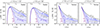Fig. 1. Axisymmetric oscillation frequencies calculated for different β and NSs with j = 0.2 and two particular values of q/j2: q/j2 = 1.5 (extreme NS compactness) and q/j2 = 10 (high NS oblateness). Left: Radial mode. Right: Vertical mode. The curves indicating particular values of β are normalised to the maximum value, β = βmax. The critical radius limiting the existence of cusp tori is denoted by the dotted vertical line marked rmc. The maximum value β = βmax matches the cusp value when r < rmc and the value implying tori extending to infinity when r > rmc. For the absolute value of β, only one specific curve is drawn in each panel, $\beta =\sqrt{0.15}$ (marked in grey), which makes it possible to distinguish frequencies that correspond to relatively large tori, as they are displayed below this curve. The dotted vertical lines in each panel marked rmc denote the radii limiting the existence of cusp tori: any torus with a centre above this radius does not exhibit a cusp. An analogous notation is used later in several other figures.

In a full analogy to the left panel of Fig. 1, the right panel compares the axisymmetric (m = 0) vertical mode frequencies for tori with different thicknesses and NSs with j = 0.2 and different levels of compactness. Again, the frequencies behave qualitatively like a test-particle vertical epicyclic frequency, while the pressure corrections are negative. A more detailed quantitative comparison is provided in Fig. A.2.

6.2. Radial precession (m = −1 radial mode)

The left panel of Fig. 2 compares the radial precession mode frequencies for tori with different thicknesses and NSs with j = 0.2 and different levels compactness. For radii close to the ISCO, the pressure corrections are negative. The highest precession frequency is achieved at r₀ = r_ISCO, where only an infinitely slender torus with zero pressure corrections can exist. The maximum achievable frequency slightly drops with rising NS quadrupole moment as the ISCO moves to larger radii, but it is still higher than the precession rate for lower q at the same (coordinate) radius.

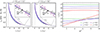Fig. 2. Behaviour of the radial precession frequency. Left: Radial precession frequencies calculated for different β and NSs with j = 0.2 and two particular values of q/j2: q/j2 = 1.5 (extreme NS compactness) and q/j2 = 10 (high NS oblateness). Right: Radial coordinates corresponding to the vanishing correction to the radial precession oscillation mode frequency, i.e. radii where ${\nu }_{\mathrm{RP}}^{(2)}=0$.

For larger radii, the corrections are smaller but can be positive, and at radii where they change sign, the frequency does not depend on the torus thickness. This feature is present for both rotating and non-rotating stars. Radii relevant to this effect are shown in the right panel of Fig. 2. A more detailed quantitative comparison between the radial precession mode frequencies is provided in Fig. B.1.

6.3. Vertical precession (m = −1 vertical mode)

The left panel of Fig. 3 compares the vertical precession mode frequencies for tori with different thicknesses and NSs with j = 0.2 and different levels of compactness. The frequency behaviour is even more complex than in the case of radial precession.

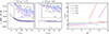Fig. 3. Behaviour of the vertical precession frequency. Left: Vertical precession frequencies calculated for different β and NSs with j = 0.2 and two particular values of q/j2: q/j2 = 1.5 (extreme NS compactness) and q/j2 = 10 (high NS oblateness). Right: Radial coordinates corresponding to the vanishing correction to the vertical precession oscillation mode frequency, i.e. radii where ${\nu }_{\mathrm{LT}}^{(2)}=0$.

For compact stars, the highest frequencies are achieved at the ISCO. For the test-particle motion and a high NS oblateness, the combined influence of the oblate shape of the star and frame-dragging induces non-monotonic frequency profiles with a maximum above the ISCO and with the emergence of a zero-frequency radius at which the precession changes its orientation (Kluźniak & Rosińska 2013, 2014; Tsang & Pappas 2016; Urbancová et al. 2019). The same occurs for slender and non-slender tori. At the same time, the correction to the mode frequency exhibits a behaviour similar to the case of radial precession, and radii at which the correction changes its sign exist. The relevant radii are shown in the right panel of Fig. 3.

A more detailed quantitative comparison between the vertical precession mode frequencies is provided in Fig. B.2, and an extended discussion of the mode frequency behaviour is given in Sect. 8.4.

7. Approximate relations

The formulae for the oscillation and precession frequencies investigated in the previous section are presented in our public codes. Their explicit forms are lengthy and potentially too complicated for practical calculations. Inspired by our previous work (Török et al. 2022), we provide their approximate versions, which enable a more efficient implementation.

For each of the four modes, we postulate an approximate formula that in the limit of a slender torus provides frequencies of free test-particle motion, and in the limit of a marginally overflowing (cusp) torus fits the results of the exact calculations of the mode frequency well. The numerical coefficients in the approximate formula were found by comparing them with the results of the exact mode frequency calculations, which were performed using the least-squares method. Expressions that allow us to calculate tori with a general thickness are also included.

7.1. Axisymmetric radial mode

The axisymmetric radial mode frequency can be approximated as

$$\begin{array}{c}\hfill {\nu }_{\mathrm{R}}={\nu }_K\mathcal{R}\sqrt{1-6{\mathcal{V}}_0^{2/3}+8j{\mathcal{V}}_0+57j^2{\mathcal{V}}_0^{7/3}-3q\mathcal{Q}},\end{array}$$(29)

where

$$\begin{array}{cc}\hfill {\mathcal{V}}_0& \equiv \frac{{\nu }_{\mathrm{K}}/{\nu }_0}{6^{3/2}-j{\nu }_{\mathrm{K}}/{\nu }_0-\frac{1}{2}(j^2-q){({\nu }_{\mathrm{K}}/{\nu }_0)}^2},{\nu }_0=2198\frac{{\mathrm{M}}_{\odot }}{M},\hfill \\ \hfill \mathcal{Q}& ={\mathcal{V}}_0^{4/3}(1+19{\mathcal{V}}_0).\hfill \end{array}$$(30)

Here, ν₀ is the Keplerian frequency at the ISCO evaluated for a non-rotating star.

7.1.1. Geodesic limit versus limit of the cusp torus

For ℛ = 1, our formula gives the radial epicyclic frequency of a free test particle. Choosing

$$\begin{array}{c}\hfill \mathcal{R}=\frac{32}{33}-\frac{10{({\mathcal{V}}_0^{-1}-18.4+15j-4q)}^2}{{\nu }_0(1-1.5j+0.6q)},\end{array}$$(31)

we obtain a relation for the axisymmetric radial oscillations of a torus with a cusp. The specific ℛ function takes values between 0 and 1. Its dependence on the space-time parameters is illustrated in Fig. 4a, while a comparison between the (exact) mode frequencies and the approximate relation is shown in Fig. 4b, assuming very slowly rotating stars. A thorough comparison between the outcomes of the exact calculations and the application of the approximate relation across the whole considered range of parameters is provided in Fig. C.1.

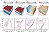Fig. 4. Values of specific functions used in approximate relations (top) and comparison between the exact solution and the approximate relations in the case of very slowly rotating NSs (bottom). Panels a and b: Axisymmetric radial mode. Panels c and d: Axisymmetric vertical mode. Panels e and f: Radial precession mode. Panels g and h: Vertical precession mode. The frequencies are normalised with respect to their highest values, νmax.

7.1.2. Tori of arbitrary thicknesses

To describe oscillation frequencies of tori of an arbitrary thickness, we used

$$\begin{array}{c}\hfill \mathcal{R}=1-{\left(\frac{\beta }{{\beta }_{\mathrm{cusp}}}\right)}^2(\frac{1}{33}+\frac{10{({\mathcal{V}}_0^{-1}-18.4+15j-4q)}^2}{{\nu }_0(1-1.5j+0.6q)}).\end{array}$$(32)

7.2. Axisymmetric vertical mode

The axisymmetric vertical mode frequency can be approximated as

$$\begin{array}{c}\hfill {\nu }_{\mathrm{V}}={\nu }_K\mathcal{K}\sqrt{1-4j{\mathcal{V}}_0-24j^2{\mathcal{V}}_0^{7/3}+3q{\mathcal{V}}_0^{4/3}(1+8{\mathcal{V}}_0)}.\end{array}$$(33)

7.2.1. Geodesic limit versus limit of the cusp torus

For 𝒦 = 1, our formula provides the value of the vertical epicyclic frequency of a free test particle. Choosing

$$\begin{array}{c}\hfill \mathcal{K}=1-\frac{14{({\mathcal{V}}_0^{-1}-\frac{40}{3}+10j-2.5q)}^2}{{\nu }_0(1-1.7j+0.7q)},\end{array}$$(34)

we obtain an approximate relation for the frequencies of a torus with a cusp, where 𝒦 ∈ (0,  1). The dependence of the specific 𝒦 function on the space-time parameters is illustrated in Fig. 4, while a comparison between the (exact) mode frequencies and the approximate relation is shown in Fig. 4, assuming very slowly rotating stars. A thorough comparison between the outcomes of the exact calculations and the application of the approximate relation across the whole range of considered parameters is provided in Fig. C.2.

7.2.2. Tori of arbitrary thicknesses

The frequencies of tori of an arbitrary thickness can be evaluated using

$$\begin{array}{c}\hfill \mathcal{K}=1-{\left(\frac{\beta }{{\beta }_{\mathrm{cusp}}}\right)}^2\left(\frac{14{({\mathcal{V}}_0^{-1}-\frac{40}{3}+10j-2.5q)}^2}{{\nu }_0(1-1.7j+0.7q)}\right).\end{array}$$(35)

7.3. Radial precession (non-axisymmetric radial mode)

The radial precession frequency can be approximated as (Török et al. 2022)

$$\begin{array}{c}\hfill {\nu }_{\mathrm{RP}}={\nu }_{\mathrm{K}}[1-\mathcal{B}\sqrt{1-6{\mathcal{V}}_0^{2/3}+8j{\mathcal{V}}_0+57j^2{\mathcal{V}}_0^{7/3}-3q\mathcal{Q}}].\end{array}$$(36)

7.3.1. Geodesic limit versus limit of the cusp torus

Choosing a constant ℬ, ℬ = 1, our relation provides the value of the periastron precession frequency of the test-particle motion around oblate NSs with very high accuracy. When we choose

$$\begin{array}{c}\hfill \mathcal{B}=0.8-0.2j,\end{array}$$(37)

the resulting relation matches the numerical findings for the cusp torus radial precession well. The specific ℬ function does not depend on the Keplerian frequency (radial coordinate r), unlike the case of the axisymmetric modes. For slowly rotating stars, it takes values close to ℬ = 0.75. The exact values are illustrated in Fig. 4e, while a comparison between the (exact) mode frequencies and the approximate relation is shown in Fig. 4f, assuming very slowly rotating stars. A thorough comparison between the outcomes of the exact calculations and the application of the approximate relation across the whole considered range of parameters is provided in Fig. C.3.

7.3.2. Tori of arbitrary thicknesses

We determined the relevant precession frequency for tori of an arbitrary thickness by choosing

$$\begin{array}{c}\hfill \mathcal{B}=1-0.2(1+j){\left(\frac{\beta }{{\beta }_{\mathrm{cusp}}}\right)}^2.\end{array}$$(38)

7.4. Vertical precession

The vertical precession frequency can be approximated as

$$\begin{array}{c}\hfill {\nu }_{\mathrm{LT}}={\nu }_K\mathcal{T}\sqrt{1-4j{\mathcal{V}}_0-24j^2{\mathcal{V}}_0^{7/3}+3q{\mathcal{V}}_0^{4/3}(1+8{\mathcal{V}}_0)}.\end{array}$$(39)

7.4.1. Geodesic limit versus limit of the cusp torus

Choosing 𝒯 = 1, our formula provides the value of the vertical precession frequency for a free test particle. Selecting

$$\begin{array}{cc}\hfill \mathcal{T}=& 1-\frac{5j}{{\nu }_0}[1-\frac{2{({\mathcal{V}}_0^{-2/3}-6.1+2.5j)}^2}{1-2j-2j^2+q}]\hfill \\ \hfill & +\frac{9}{{\nu }_0}(q-j^2)({\mathcal{V}}_0^{-2/3}-7.2),\hfill \end{array}$$(40)

we can describe the vertical precession of a cusp torus. The specific 𝒯 function takes values very close to 1. The exact values are illustrated in Fig. 4g, while a comparison between the (exact) mode frequencies and the approximate relation is shown in Fig. 4h, assuming very slowly rotating stars. A thorough comparison between the outcomes of the exact calculations and the application of the approximate relation across the whole considered range of parameters is provided in Fig. C.4.

7.4.2. Tori of arbitrary thicknesses

To describe a torus of arbitrary thickness, we used

$$\begin{array}{cc}\hfill \mathcal{T}=& 1-{\left(\frac{\beta }{{\beta }_{\mathrm{cusp}}}\right)}^2\{\frac{5j}{{\nu }_0}[1-\frac{2{({\mathcal{V}}_0^{-2/3}-6.1+2.5j)}^2}{1-2j-2j^2+q}]\hfill \\ \hfill & +\frac{9}{{\nu }_0}(q-j^2)({\mathcal{V}}_0^{-2/3}-7.2)\}.\hfill \end{array}$$(41)

8. Discussion and conclusions

The impact of the torus thickness leads, in most cases, to relatively high negative corrections to the mode frequencies, which should be reflected within possible astrophysical applications. Furthermore, as found in Sects. 6.2 and 6.3, the pressure corrections for the precession modes can be positive within a limited range of radii because special radii exist at which the precession frequency does not depend on the torus thickness. This can have observable consequences. Nevertheless, since we are constrained by the adopted perturbative approach and the effect manifests itself at a relatively large radius at which the scatter between the frequencies calculated for different tori is generally very small, it will be useful to verify its presence using a suitable future numerical solution of Eq. (8).

8.1. Influence of NS parameters

Both the NS rotation and rotationally induced oblateness affecting the angular momentum and quadrupole moment of the NS significantly affect the frequencies of the investigated torus oscillations. The impact of the quadratic relations behind the nature of the modes is well illustrated in terms of the quadrupole parameter, q/j², used in our study, which for an NS with a given EoS and mass does not depend on the NS rotational frequency (Hartle & Thorne 1968; Urbancová et al. 2019). This parameter effectively ranges from q/j² ∼ 1.5 to q/j² ∼ 10 and determines whether the influence of the t − ϕ component of the metric tensor and related frame-dragging effects dominate (low values of the parameter correspond to a Kerr-like behaviour) or are overwhelmed by the other components (high values of the parameter correspond to the effective suppression of frame-dragging effects by the NS oblateness).

This interaction between the relativistic frame-dragging effects associated with the angular momentum and the effects associated with the quadrupole moment, which would also arise in Newtonian physics, determines the resulting behaviour of the frequencies of the studied modes. For low values of q/j², the highest frequencies of the modes increase with j within the considered range. For high values of q/j², these frequencies increase only very little or even decrease with increasing j.

8.2. Consequences for models of NS variability: HF QPOs

Török et al. (2016, 2022) have introduced a QPO model that identifies the twin peak QPO frequencies with the Keplerian frequency, ν_K = Ω₀/2π, and the radial precession frequency, ν_RP, of the fluid in the cusp-torus configuration (the CT model). In the left panel of Fig. 5, we compare the best fits to the frequencies observed in the atoll source 4U 1636−53 (the data are taken from Barret et al. 2006; Török 2009) obtained using the CT model to the best fits based on the relativistic precession (RP) model (Stella & Vietri 1999; Stella et al. 1999).

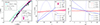Fig. 5. Response of precession frequencies to changes in NS parameters. Left: Correlations between the lower and upper QPO frequencies, νL and νU, predicted by the CT and RP models, compared to the observed data from the atoll source 4U 1636−53. The best fits predicted for non-rotating NSs are denoted by thick solid lines, while the best fits for moderately rotating NSs with j = 0.22 and q = 6j2 are denoted by dashed lines. The thin solid lines show these values of M and j but different values of q (q = 1.5j2). For the CT model, the light-coloured region emphasises the change in the frequencies predicted by the model with changing q. Middle: Relative change in the cusp torus precession frequencies with angular momentum at the radius where νRP = 0.75 νK. Within the RP and CT models, this radius corresponds to the bottom-left group of data points shown in the left panel. The light-coloured region emphasises the corresponding change in νRP. Right: Relative change in the precession frequencies with the quadrupole parameter. The frequencies are calculated at the same radius as in the middle panel.

Figure 5 shows that the RP model, which deals with geodesic precession, provides less promising fits of the data than the CT model. The effects associated with the NS rotation do not bring significant improvement in comparison to the non-rotating case and instead change the best-fitting mass value because the fitting-parameter space is almost degenerate (Török et al. 2016, 2022). Moreover, when we restrict ourselves to values of the Hartle-Thorne space-time parameters that are consistent with current NS models or impose even tighter constraints, such as j < 0.3, M < 2.3 M_⊙ and q/j² < 10, no conceivable smooth monotonic curve can reproduce the data in a significantly better way than the CT model.

8.3. Consequences for models of NS variability: LF QPOs

In principle, the relations derived here, including those determining the vertical precession frequency, can be used in an analogous way to place constraints on models of LF QPOs, providing that they are associated with vertical precession. It can be very promising to follow this research direction, which was initiated in the context of the RP model. In the middle and right panels of Fig. 5, we consider a particular orbital radius where ν_RP = 0.75 ν_K. Within the RP and CT models, this radius roughly corresponds to a large part of the documented QPO detections (r = 6.75 r_G when j = 0). These panels clearly illustrate that the vertical precession frequency of the cusp torus is more sensitive to the angular momentum and quadrupole moment than the radial precession frequency. This is caused by the strong vertical change in the gravitational field in the vicinity of an oblate NS, which already affects the test-particle motion (Morsink & Stella 1999; Kluźniak & Rosińska 2013) and then applies to the fluid motion in tori of any thickness.

To explore detailed consequences of the behaviour of ν_LT in relation to QPO models and diagnostics of NS parameters, further investigation is needed. As shown in the middle panel of Fig. 5, the dependence of ν_LT on the NS spin can (for test particles and fluid motion) exhibit a clear maximum, which can be of astrophysical importance.

8.4. Impact of NS EoS

We have focused so far on examining the effects of the space-time parameters on the investigated oscillations while taking a range of these parameters associated with present models of NSs into account. As follows from the results of Paper I, particular astrophysical applications of our formulae should be rather sensitive to the NS EoS, notably the specific position of the NS surface.

An example of the impact of the NS EoS choice can be demonstrated by the effect of the orientation change in the vertical precession discussed in Sect. 6.3. In the left panel of Fig. 6, we illustrate profiles of the vertical precession frequency for a particular choice of space-time parameter values along with several related NS radii that were calculated using the L NS EoS introduced by Pandharipande & Smith (1975). The figure shows that the investigated effect occurs at radii that are not necessarily above the NS surface. We used the L NS EoS as it is extremely stiff and therefore allows us to illustrate the effect of a large quadrupole moment well, but the effect can be relevant for many currently considered EoS.

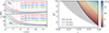Fig. 6. Impact of the equation of state on the vanishing of vertical precession frequency. Left: Profiles of the vertical precession frequency of the slender torus for a particular choice of space-time parameter values, along with the related NS radii calculated using the L NS EoS (Pandharipande & Smith 1975) and denoted by dashed vertical lines. The top (bottom) panel corresponds to a rotational frequency of 400 Hz (500 Hz). Right: Range of the Hartle-Thorne space-time parameters in which the vertical precession can change orientation. The thick black line marked β = 0 indicates the limiting NS parameters relevant for the case of a slender torus, which are the same as for the geodesic (thin-disc) case explored by Tsang & Pappas (2016). The shaded region below the β = 0 line is the area in which this effect can occur, but the corresponding torus overlaps with the NS surface. The coloured region above the β = 0 line corresponds to tori that do not overlap with the star, and the colour scale indicates the radii of their centres for the slender-torus case. In full analogy, the lines for β = 0.1 and β = 0.2 show the limiting parameters where the torus of the corresponding thickness would touch the NS surface. In these cases, the corresponding r0 colour maps would be slightly different but still almost identical to the β = 0 map shown in this figure.

In the right panel of Fig. 6, we show the full range of the NS angular momentum and quadrupole moment, which corresponds to this effect. Using the recently identified universal relations (Maselli et al. 2013; Urbanec et al. 2013; Yagi & Yunes 2013a,b; Pappas 2015; Reina et al. 2017), we denote the area that determines the range limited by the condition that the inner edge of the torus must be located above the NS surface. Clearly, this range is smaller than the full range given when considering the Hartle-Thorne metric alone.

8.5. Summary and overall implications

We studied the epicyclic oscillations of fluid tori in the Hartle-Thorne geometry, with special attention to the two axisymmetric and two precession modes. We focused on the case of discs with a constant angular momentum distribution and polytropic index n = 3⁴. We conclude that the quadrupole moment induced by the NS rotation likely strongly affects various astrophysical phenomena involving oscillations of the accreted fluid, such as the observed HF and LF QPOs. The formulae derived in our work can help us quantify this impact. While here we provide all the formulae required for a further examination of the underlying parameter space, particular astrophysical applications that might restrict the dense-matter EoS will need to be conceived, focusing on specific NS models.

Acknowledgments

We thank Marek Abramowicz, Omer Blaes, and Włodek Kluźniak for the valuable discussions. We wish to express our gratitude to the University of California in Santa Barbara for hosting us while this study was being initiated. We also thank the reviewer for valuable comments and suggestions, which significantly helped to improve the paper. We acknowledge the Czech Science Foundation (GAČR) grant No. 21-06825X and the INTER-EXCELLENCE project No. LTI17018, and the PRODEX program of the European Space Agency (ref. 4000132152). The INTER-EXCELLENCE project No. LTT17003 is acknowledged by KK, and the INTER-EXCELLENCE project No. LTC18058 is acknowledged by MM and MU. VK acknowledges the Research Infrastructure LM2023047 of the Czech Ministry of Education, Youth and Sports. OS acknowledges funding by the Deutsche Forschungsgemeinschaft (DFG, German Research Foundation) under Germany’s Excellence Strategy – EXC 2094 – 390783311. We furthermore acknowledge the support provided by the internal grants of Silesian University, SGS/31/2023 and SGS/25/2024.

References

Appendix A: Frequencies of axisymmetric modes: Detailed view

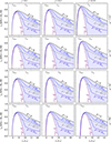Fig. A.1. Axisymmetric radial oscillation frequencies of tori with different β plotted for the NS dimensionless angular momentum (j = 0.1, j = 0.2 and j = 0.35) and its dimensionless quadrupole parameter (q/j2 = 1.5 – extreme compactness, q/j2 = 3 – small oblateness, q/j2 = 6 – moderate oblateness and q/j2 = 10 – large oblateness).

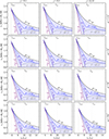Fig. A.2. Axisymmetric vertical epicyclic frequencies of tori with different β plotted for different values of NS dimensionless angular momentum (j = 0.1, j = 0.2 and j = 0.35) and the quadrupole parameter (q/j2 = 1.5 – extreme compactness, q/j2 = 3 – small oblateness, q/j2 = 6 – moderate oblateness and q/j2 = 10 – large oblateness).

Appendix B: Frequencies of non-axisymmetric modes: Detailed view

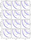Fig. B.1. Radial precession frequencies of tori with different β plotted for different values of NS angular momentum (j = 0.1, j = 0.2 and j = 0.35) and the quadrupole parameter (q/j2 = 1.5 – extreme compactness, q/j2 = 3 – small oblateness, q/j2 = 6 – moderate oblateness and q/j2 = 10 – large oblateness).

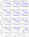Fig. B.2. Vertical precession frequencies of tori with different β for NS angular momentum (j = 0.1, j = 0.2 and j = 0.35) and its dimensionless quadrupole parameter (q/j2 = 1.5 – extreme compactness, q/j2 = 3 – small oblateness, q/j2 = 6 – moderate oblateness and q/j2 = 10 – large oblateness).

Appendix C: Approximative relations: Detailed view

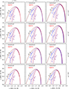Fig. C.1. Comparison of the radial epicyclic frequency of tori with different thicknesses (solid) and the approximation relations (dashed).

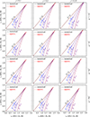Fig. C.2. Comparison of the vertical epicyclic frequency of tori with different thicknesses (solid) and the approximation relations (dashed).

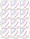Fig. C.3. Comparison of the radial precession frequency of tori with different thicknesses (solid) and the approximation relations (dashed).

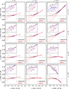Fig. C.4. Comparison of the vertical precession frequency of tori with different thicknesses (solid) and the approximation relations (dashed).

Appendix D: Impact of a change in the polytropic index

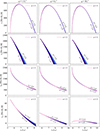Fig. D.1. Frequencies of axisymmetric oscillations and precession frequencies of cusp tori as a function of the polytropic index for j = 0.2. Frequency values corresponding to the range n ∈ [1.5,  3.5] are scaled in shades of blue. The value of n = 3 is emphasised by purple.

All Figures

Fig. 1. Axisymmetric oscillation frequencies calculated for different β and NSs with j = 0.2 and two particular values of q/j2: q/j2 = 1.5 (extreme NS compactness) and q/j2 = 10 (high NS oblateness). Left: Radial mode. Right: Vertical mode. The curves indicating particular values of β are normalised to the maximum value, β = βmax. The critical radius limiting the existence of cusp tori is denoted by the dotted vertical line marked rmc. The maximum value β = βmax matches the cusp value when r < rmc and the value implying tori extending to infinity when r > rmc. For the absolute value of β, only one specific curve is drawn in each panel, $\beta =\sqrt{0.15}$ (marked in grey), which makes it possible to distinguish frequencies that correspond to relatively large tori, as they are displayed below this curve. The dotted vertical lines in each panel marked rmc denote the radii limiting the existence of cusp tori: any torus with a centre above this radius does not exhibit a cusp. An analogous notation is used later in several other figures.

In the text

Fig. 2. Behaviour of the radial precession frequency. Left: Radial precession frequencies calculated for different β and NSs with j = 0.2 and two particular values of q/j2: q/j2 = 1.5 (extreme NS compactness) and q/j2 = 10 (high NS oblateness). Right: Radial coordinates corresponding to the vanishing correction to the radial precession oscillation mode frequency, i.e. radii where ${\nu }_{\mathrm{RP}}^{(2)}=0$.

In the text

Fig. 3. Behaviour of the vertical precession frequency. Left: Vertical precession frequencies calculated for different β and NSs with j = 0.2 and two particular values of q/j2: q/j2 = 1.5 (extreme NS compactness) and q/j2 = 10 (high NS oblateness). Right: Radial coordinates corresponding to the vanishing correction to the vertical precession oscillation mode frequency, i.e. radii where ${\nu }_{\mathrm{LT}}^{(2)}=0$.

In the text

Fig. 4. Values of specific functions used in approximate relations (top) and comparison between the exact solution and the approximate relations in the case of very slowly rotating NSs (bottom). Panels a and b: Axisymmetric radial mode. Panels c and d: Axisymmetric vertical mode. Panels e and f: Radial precession mode. Panels g and h: Vertical precession mode. The frequencies are normalised with respect to their highest values, νmax.

In the text

Fig. 5. Response of precession frequencies to changes in NS parameters. Left: Correlations between the lower and upper QPO frequencies, νL and νU, predicted by the CT and RP models, compared to the observed data from the atoll source 4U 1636−53. The best fits predicted for non-rotating NSs are denoted by thick solid lines, while the best fits for moderately rotating NSs with j = 0.22 and q = 6j2 are denoted by dashed lines. The thin solid lines show these values of M and j but different values of q (q = 1.5j2). For the CT model, the light-coloured region emphasises the change in the frequencies predicted by the model with changing q. Middle: Relative change in the cusp torus precession frequencies with angular momentum at the radius where νRP = 0.75 νK. Within the RP and CT models, this radius corresponds to the bottom-left group of data points shown in the left panel. The light-coloured region emphasises the corresponding change in νRP. Right: Relative change in the precession frequencies with the quadrupole parameter. The frequencies are calculated at the same radius as in the middle panel.

In the text

Fig. 6. Impact of the equation of state on the vanishing of vertical precession frequency. Left: Profiles of the vertical precession frequency of the slender torus for a particular choice of space-time parameter values, along with the related NS radii calculated using the L NS EoS (Pandharipande & Smith 1975) and denoted by dashed vertical lines. The top (bottom) panel corresponds to a rotational frequency of 400 Hz (500 Hz). Right: Range of the Hartle-Thorne space-time parameters in which the vertical precession can change orientation. The thick black line marked β = 0 indicates the limiting NS parameters relevant for the case of a slender torus, which are the same as for the geodesic (thin-disc) case explored by Tsang & Pappas (2016). The shaded region below the β = 0 line is the area in which this effect can occur, but the corresponding torus overlaps with the NS surface. The coloured region above the β = 0 line corresponds to tori that do not overlap with the star, and the colour scale indicates the radii of their centres for the slender-torus case. In full analogy, the lines for β = 0.1 and β = 0.2 show the limiting parameters where the torus of the corresponding thickness would touch the NS surface. In these cases, the corresponding r0 colour maps would be slightly different but still almost identical to the β = 0 map shown in this figure.

In the text

	Fig. A.1. Axisymmetric radial oscillation frequencies of tori with different β plotted for the NS dimensionless angular momentum (j = 0.1, j = 0.2 and j = 0.35) and its dimensionless quadrupole parameter (q/j2 = 1.5 – extreme compactness, q/j2 = 3 – small oblateness, q/j2 = 6 – moderate oblateness and q/j2 = 10 – large oblateness).
In the text

	Fig. A.2. Axisymmetric vertical epicyclic frequencies of tori with different β plotted for different values of NS dimensionless angular momentum (j = 0.1, j = 0.2 and j = 0.35) and the quadrupole parameter (q/j2 = 1.5 – extreme compactness, q/j2 = 3 – small oblateness, q/j2 = 6 – moderate oblateness and q/j2 = 10 – large oblateness).
In the text

	Fig. B.1. Radial precession frequencies of tori with different β plotted for different values of NS angular momentum (j = 0.1, j = 0.2 and j = 0.35) and the quadrupole parameter (q/j2 = 1.5 – extreme compactness, q/j2 = 3 – small oblateness, q/j2 = 6 – moderate oblateness and q/j2 = 10 – large oblateness).
In the text

	Fig. B.2. Vertical precession frequencies of tori with different β for NS angular momentum (j = 0.1, j = 0.2 and j = 0.35) and its dimensionless quadrupole parameter (q/j2 = 1.5 – extreme compactness, q/j2 = 3 – small oblateness, q/j2 = 6 – moderate oblateness and q/j2 = 10 – large oblateness).
In the text

	Fig. C.1. Comparison of the radial epicyclic frequency of tori with different thicknesses (solid) and the approximation relations (dashed).
In the text

	Fig. C.2. Comparison of the vertical epicyclic frequency of tori with different thicknesses (solid) and the approximation relations (dashed).
In the text

	Fig. C.3. Comparison of the radial precession frequency of tori with different thicknesses (solid) and the approximation relations (dashed).
In the text

	Fig. C.4. Comparison of the vertical precession frequency of tori with different thicknesses (solid) and the approximation relations (dashed).
In the text

	Fig. D.1. Frequencies of axisymmetric oscillations and precession frequencies of cusp tori as a function of the polytropic index for j = 0.2. Frequency values corresponding to the range n ∈ [1.5,  3.5] are scaled in shades of blue. The value of n = 3 is emphasised by purple.
In the text

References

- Abramowicz, M. A., & Kluźniak, W. 2001, A&A, 374, L19 [NASA ADS] [CrossRef] [EDP Sciences] [Google Scholar]
- Abramowicz, M. A., Karas, V., Kluźniak, W., Lee, W. H., & Rebusco, P. 2003a, PASJ, 55, 467 [NASA ADS] [CrossRef] [Google Scholar]
- Abramowicz, M. A., Bulik, T., Bursa, M., & Kluźniak, W. 2003b, A&A, 404, L21 [NASA ADS] [CrossRef] [EDP Sciences] [Google Scholar]
- Abramowicz, M. A., Blaes, O. M., Horák, J., Kluźniak, W., & Rebusco, P. 2006, Class. Quant. Grav., 23, 1689 [NASA ADS] [CrossRef] [Google Scholar]
- Alpar, M. A., & Shaham, J. 1985, Nature, 316, 239 [NASA ADS] [CrossRef] [Google Scholar]
- Bachetti, M., Romanova, M. M., Kulkarni, A., Burderi, L., & di Salvo, T. 2010, MNRAS, 403, 1193 [NASA ADS] [CrossRef] [Google Scholar]
- Barret, D., Olive, J.-F., & Miller, M. C. 2006, MNRAS, 370, 1140 [NASA ADS] [CrossRef] [Google Scholar]
- Blaes, O. M. 1987, MNRAS, 227, 975 [NASA ADS] [Google Scholar]
- Blaes, O. M., Arras, P., & Fragile, P. C. 2006, MNRAS, 369, 1235 [NASA ADS] [CrossRef] [Google Scholar]
- Bursa, M. 2005, Astron. Nachr., 326, 849 [NASA ADS] [CrossRef] [Google Scholar]
- Čadež, A., Calvani, M., & Kostić, U. 2008, A&A, 487, 527 [NASA ADS] [CrossRef] [EDP Sciences] [Google Scholar]
- de Avellar, M. G. B., Porth, O., Younsi, Z., & Rezzolla, L. 2018, MNRAS, 474, 3967 [NASA ADS] [CrossRef] [Google Scholar]
- Dönmez, O., Zanotti, O., & Rezzolla, L. 2011, MNRAS, 412, 1659 [CrossRef] [Google Scholar]
- Faraji, S., & Trova, A. 2023, MNRAS, 525, 1126 [NASA ADS] [CrossRef] [Google Scholar]
- Fragile, P. C., Straub, O., & Blaes, O. 2016, MNRAS, 461, 1356 [NASA ADS] [CrossRef] [Google Scholar]
- Frank, J., King, A., & Raine, D. J. 2002, Accretion Power in Astrophysics: Third Edition (Cambridge: Cambridge University Press) [Google Scholar]
- Germanà, C. 2017, Phys. Rev. D, 96, 103015 [CrossRef] [Google Scholar]
- Hartle, J. B. 1967, ApJ, 150, 1005 [NASA ADS] [CrossRef] [Google Scholar]
- Hartle, J. B., & Thorne, K. S. 1968, ApJ, 153, 807 [NASA ADS] [CrossRef] [Google Scholar]
- Huang, C.-Y., Ye, Y.-C., Wang, D.-X., & Li, Y. 2016, MNRAS, 457, 3859 [CrossRef] [Google Scholar]
- Kato, S. 2001, PASJ, 53, 1 [NASA ADS] [CrossRef] [Google Scholar]
- Kato, S., Fukue, J., & Mineshige, S. 2008, Black-Hole Accretion Disks: Towards a New Paradigm (Kyoto: Kyoto University Press) [Google Scholar]
- Kluźniak, W., & Abramowicz, M. A. 2001a, Acta Phys. Polonica B, 32, 3605 [Google Scholar]
- Kluźniak, W., & Abramowicz, M. A. 2001b, ArXiv e-prints [arXiv:astroph/0105057] [Google Scholar]
- Kluźniak, W., & Rosińska, D. 2013, MNRAS, 434, 2825 [CrossRef] [Google Scholar]
- Kluźniak, W., & Rosińska, D. 2014, J. Phys. Conf. Ser., 496, 012016 [CrossRef] [Google Scholar]
- Kluźniak, W., Abramowicz, M. A., Kato, S., Lee, W. H., & Stergioulas, N. 2004, ApJ, 603, L89 [CrossRef] [Google Scholar]
- Kotrlová, A., Šrámková, E., Török, G., et al. 2020, A&A, 643, A31 [NASA ADS] [CrossRef] [EDP Sciences] [Google Scholar]
- Lamb, F. K., Shibazaki, N., Alpar, M. A., & Shaham, J. 1985, Nature, 317, 681 [NASA ADS] [CrossRef] [Google Scholar]
- Lattimer, J. M., & Prakash, M. 2007, Phys. Rep., 442, 109 [Google Scholar]
- Le, T., Wood, K. S., Wolff, M. T., Becker, P. A., & Putney, J. 2016, ApJ, 819, 112 [NASA ADS] [CrossRef] [Google Scholar]
- Maselli, A., Cardoso, V., Ferrari, V., Gualtieri, L., & Pani, P. 2013, Phys. Rev. D, 88, 023007 [NASA ADS] [CrossRef] [Google Scholar]
- Matuszková, M., Török, G., Lančová, D., et al. 2024, A&A, 691, A167 [NASA ADS] [CrossRef] [EDP Sciences] [Google Scholar]
- Miller, M. C., Lamb, F. K., & Psaltis, D. 1998, ApJ, 508, 791 [NASA ADS] [CrossRef] [Google Scholar]
- Morsink, S. M., & Stella, L. 1999, ApJ, 513, 827 [NASA ADS] [CrossRef] [Google Scholar]
- Mukhopadhyay, B. 2009, ApJ, 694, 387 [NASA ADS] [CrossRef] [Google Scholar]
- Pandharipande, V. R., & Smith, R. A. 1975, Phys. Lett. B, 59, 15 [NASA ADS] [CrossRef] [Google Scholar]
- Papaloizou, J. C. B., & Pringle, J. E. 1984, MNRAS, 208, 721 [NASA ADS] [CrossRef] [Google Scholar]
- Pappas, G. 2015, MNRAS, 454, 4066 [NASA ADS] [CrossRef] [Google Scholar]
- Pétri, J. 2005, A&A, 439, L27 [NASA ADS] [CrossRef] [EDP Sciences] [Google Scholar]
- Psaltis, D., Wijnands, R., Homan, J., et al. 1999, ApJ, 520, 763 [NASA ADS] [CrossRef] [Google Scholar]
- Reina, B., Sanchis-Gual, N., Vera, R., & Font, J. A. 2017, MNRAS, 470, L54 [CrossRef] [Google Scholar]
- Rezzolla, L., Yoshida, S., & Zanotti, O. 2003a, MNRAS, 344, 978 [NASA ADS] [CrossRef] [Google Scholar]
- Rezzolla, L., Yoshida, S., Maccarone, T. J., & Zanotti, O. 2003b, MNRAS, 344, L37 [CrossRef] [Google Scholar]
- Smith, K. L., Tandon, C. R., & Wagoner, R. V. 2021, ApJ, 906, 92 [NASA ADS] [CrossRef] [Google Scholar]
- Šrámková, E., Torkelsson, U., & Abramowicz, M. A. 2007, A&A, 467, 641 [NASA ADS] [CrossRef] [EDP Sciences] [Google Scholar]
- Stella, L., & Vietri, M. 1999, Phys. Rev. Lett., 82, 17 [NASA ADS] [CrossRef] [Google Scholar]
- Stella, L., Vietri, M., & Morsink, S. M. 1999, ApJ, 524, L63 [CrossRef] [Google Scholar]
- Straub, O., & Šrámková, E. 2009, Class. Quant. Grav., 26, 055011 [NASA ADS] [CrossRef] [Google Scholar]
- Stuchlík, Z., & Kološ, M. 2014, Phys. Rev. D, 89, 065007 [CrossRef] [Google Scholar]
- Stuchlík, Z., Kološ, M., Kovář, J., Slaný, P., & Tursunov, A. 2020, Universe, 6, 26 [Google Scholar]
- Titarchuk, L., & Wood, K. 2002, ApJ, 577, L23 [NASA ADS] [CrossRef] [Google Scholar]
- Török, G. 2009, A&A, 497, 661 [NASA ADS] [CrossRef] [EDP Sciences] [Google Scholar]
- Török, G., Abramowicz, M. A., Kluźniak, W., & Stuchlík, Z. 2005, A&A, 436, 1 [NASA ADS] [CrossRef] [EDP Sciences] [Google Scholar]
- Török, G., Goluchová, K., Horák, J., et al. 2016, MNRAS, 457, L19 [CrossRef] [Google Scholar]
- Török, G., Kotrlová, A., Matuszková, M., et al. 2022, ApJ, 929, 28 [CrossRef] [Google Scholar]
- Tsang, D., & Pappas, G. 2016, ApJ, 818, L11 [NASA ADS] [CrossRef] [Google Scholar]
- Urbancová, G., Urbanec, M., Török, G., et al. 2019, ApJ, 877, 66 [CrossRef] [Google Scholar]
- Urbanec, M., Miller, J. C., & Stuchlík, Z. 2013, MNRAS, 433, 1903 [CrossRef] [Google Scholar]
- van der Klis, M. 2006, Compact Stellar X-ray Sources (Cambridge: Cambridge University Press), 39 [CrossRef] [Google Scholar]
- Wagoner, R. V., Silbergleit, A. S., & Ortega-Rodríguez, M. 2001, ApJ, 559, L25 [NASA ADS] [CrossRef] [Google Scholar]
- Wang, D.-H., & Zhang, C.-M. 2020, MNRAS, 497, 2893 [NASA ADS] [CrossRef] [Google Scholar]
- Wang, D.-X., Gan, Z.-M., Huang, C.-Y., & Li, Y. 2008, MNRAS, 391, 1332 [NASA ADS] [CrossRef] [Google Scholar]
- Yagi, K., & Yunes, N. 2013a, Phys. Rev. D, 88, 023009 [CrossRef] [Google Scholar]
- Yagi, K., & Yunes, N. 2013b, Science, 341, 365 [NASA ADS] [CrossRef] [Google Scholar]
- Zhang, C. 2004, A&A, 423, 401 [NASA ADS] [CrossRef] [EDP Sciences] [Google Scholar]