| Issue |
A&A
Volume 691, November 2024
|
|
|---|---|---|
| Article Number | A167 | |
| Number of page(s) | 7 | |
| Section | Astrophysical processes | |
| DOI | https://doi.org/10.1051/0004-6361/202450056 | |
| Published online | 08 November 2024 | |
Accretion tori around rotating neutron stars
I. Structure, shape, and size
1
Research Centre for Computational Physics and Data Processing, Institute of Physics, Silesian University in Opava, Bezručovo nám. 13, CZ-746 01 Opava, Czech Republic
2
Astronomical Institute of the Czech Academy of Sciences, Boční II 1401, CZ-14100 Prague, Czech Republic
3
ORIGINS Excellence Cluster, Boltzmannstr. 2, 85748 Garching, Germany
4
Max Planck Institute for Extraterrestrial Physics, Gießenbachstraße 1, 85748 Garching, Germany
⋆ Corresponding author; This email address is being protected from spambots. You need JavaScript enabled to view it.
Received:
21
March
2024
Accepted:
8
September
2024
Abstract
We present a full general relativistic analytic solution for a radiation-pressure-supported equilibrium fluid torus orbiting a rotating neutron star (NS). We applied previously developed analytical methods that include the effects of both the NS’s angular momentum and quadrupole moment in the Hartle-Thorne geometry. The structure, size, and shape of the torus are explored, with a particular focus on the critically thick solution – the cusp tori. For the astrophysically relevant range of NS parameters, we examined how our findings differ from those obtained for the Schwarzschild space-time. The solutions for rotating stars display signatures of an interplay between relativistic and Newtonian effects where the impact of the NS angular momentum and quadrupole moment are almost counterbalanced at a given radius. Nevertheless, the space-time parameters still strongly influence the size of tori, which can be shown in a coordinate-independent way. Finally, we discuss the importance of the size of the central NS which determines whether or not a surrounding torus exists. We provide a set of tools in a Wolfram Mathematica code, which establishes a basis for further investigation of the impact of the NSs’ super-dense matter equation of state on the spectral and temporal behaviour of accretion tori.
Key words: stars: neutron / accretion / accretion disks
© The Authors 2024
 Open Access article, published by EDP Sciences, under the terms of the Creative Commons Attribution License (https://creativecommons.org/licenses/by/4.0), which permits unrestricted use, distribution, and reproduction in any medium, provided the original work is properly cited.
This article is published in open access under the Subscribe to Open model. This email address is being protected from spambots. You need JavaScript enabled to view it. to support open access publication.
1. Introduction
In the close vicinity of black holes (BHs) and neutron stars (NSs), accretion processes lead to the formation of discs that emit a strong radiative power. This allows us to identify the nature of these compact objects and study their properties (see e.g. Frank et al. 2002; Kato et al. 2008). In the inner accretion region, the strong gravitational effects dominate, which affect the observed variability and spectra. They are directly dependent only on the geometry of space-time in the case of BHs, while in the case of NSs, the nature of their super-dense matter plays a role as well (see e.g. Lewin & van der Klis 2010; Lattimer & Prakash 2007).
In the last few decades, several complementary approaches to investigating the properties of accreting BHs and NSs based on observed X-ray spectra and timing behaviour have been developed and gained popularity. Promising methods include fitting the X-ray spectral continuum or relativistically broadened iron lines (Fabian et al. 2000; McClintock & Remillard 2006; Shafee et al. 2008; McClintock et al. 2011; Fabian & Vaughan 2003; Reynolds & Fabian 2008; Steiner et al. 2009, 2010; Cackett et al. 2008; Piraino et al. 2012; Miller et al. 2020). Within the time domain, the interpretation of observations of quasi-periodic oscillations (QPOs) and related proposed models are often debated (e.g. Wagoner 1999; Kato 2001; Stella et al. 1998; Čadež et al. 2008; Abramowicz & Kluźniak 2001; Rezzolla et al. 2003b,a; Bursa et al. 2004; Abramowicz et al. 2006; Blaes et al. 2006; Ingram & Done 2010; de Avellar et al. 2018; Mishra et al. 2017). Stationary disc models are commonly assumed in many approaches to investigating BH and NS properties, although it is not clear whether, in real astrophysical situations, the dynamical timescales of the phenomena studied are shorter than the viscous and thermal timescales (Qian et al. 2009; McClintock et al. 2011).
A particular class of simplified stationary solutions of accretion flows in geometrically thick discs are the radiation-pressure-supported equilibrium fluid tori, often denoted as Polish doughnuts (e.g. Kozlowski et al. 1978; Abramowicz et al. 1978; Paczyński & Abramowicz 1982), which have been intensely explored and utilised within various works that assumed rotating BHs (Abramowicz & Kluźniak 2001; Török et al. 2005; Gimeno-Soler & Font 2017; Riaz et al. 2020a,b). Here, we consider tori around rotating NSs and, for the first time, apply previously developed analytical methods to the case of the Hartle-Thorne geometry, including the effects of both the NS’s angular momentum and quadrupole moment.
We explore the structure, size, and shape of the tori around rotating NSs and examine differences from the case of Schwarzschild space-time while focusing on the critically thick solution – the cusp tori. Our study provides a basis for further astrophysical applications, for example in the study of torus oscillations in relation to QPOs observed in NS systems, as discussed in our follow-up paper (Paper II, Matuszková et al. 2024).
The present paper (Paper I) is organised as follows. Section 2 introduces the adopted space-time description. In Sect. 3, we build on earlier research on accretion tori and carry out a comprehensive analytical solution describing accretion tori around rotating NSs. This solution is then further explored within the astrophysically relevant range of space-time parameters in Sect. 4. Finally, in Sect. 5, we demonstrate the use of our formulae on various astrophysically relevant examples. We then provide the reader with a short summary and state our main concluding remarks.
2. Neutron star space-time geometry
We described the space-time surrounding axisymmetric NSs by the line element expressed in the Schwarzschild coordinates, {t, r, θ, φ},
 (1)
(1)
We used units where c = G = 1, with c being the speed of light and G the gravitational constant. To measure the distance, we used rG = GM/c2. The ( − + + + ) metric signature is employed throughout the paper.
2.1. The Hartle-Thorne geometry
The exterior solution of the Hartle-Thorne metric is characterised by three parameters: the gravitational mass, M, angular momentum, J, and quadrupole moment, Q, of the star. The dimensionless forms of the angular momentum and the quadrupole moment, j = J/M2 and q = Q/M3, are used.
The metric functions take the form (Abramowicz et al. 2003)1
![Mathematical equation: $$ \begin{aligned} \nonumber g_{tt}&= -\left( 1- \frac{2M}{r} \right) \left[ 1 + j^2 F_1 \left(r\right) + q F_2 \left(r\right) \right], \\ \nonumber g_{rr}&= \left( 1- \frac{2M}{r} \right)^{-1} \left[ 1 + j^2 G_1 \left(r\right) - q F_2 \left(r\right) \right] , \\ \nonumber g_{\theta \theta }&= \left[ 1 + j^2 H_1 \left(r\right) + q H_2 \left(r\right) \right]r^2 , \\ \nonumber g_{\varphi \varphi }&= \left[ 1 + j^2 H_1 \left(r\right) + q H_2 \left(r\right) \right] r^2\sin ^2 \theta , \\ g_{t\varphi }&= - \frac{2M^2}{r} j \sin ^2 \theta , \end{aligned} $$](/articles/aa/full_html/2024/11/aa50056-24/aa50056-24-eq2.gif) (2)
(2)
where, making use of the u = cos θ substitution, one can write
![Mathematical equation: $$ \begin{aligned} F_1\left(r\right)&= - [ 8Mr^4(r-2M) ]^{-1}\nonumber \\&\quad [ u^2 ( 48M^6 - 8M^5r - 24M^4r^2 - 30M^3r^3 - 60M^2r^4 \nonumber \\&\quad + 135Mr^5 - 45r^6 ) + (r-M) ( 16M^5 + 8M^4r \nonumber \\ &\quad - 10M^2r^3 - 30Mr^4 + 15r^5 ) ] + A_1(r), \nonumber \\ F_2\left(r\right)&= \left[ 8Mr (r-2M) \right]^{-1} \nonumber \\&\quad [ 5 (3u^2 - 1) (r-M) ( 2M^2 + 6Mr - 3r^2 ) ] - A_1\left(r\right), \nonumber \\ G_1\left(r\right)&= [ 8Mr (r-2M) ]^{-1} \nonumber \\&\quad [ ( L\left(r\right) - 72M^5r ) - 3u^2 ( L\left(r\right) - 56M^5r ) ] - A_1\left(r\right), \nonumber \\ L\left(r\right)&= 80 M^6 + 8M^4r^2 + 10M^3r^3 + 20M^2r^4 - 45Mr^5 + 15r^6, \nonumber \\ A_1\left(r\right)&= \frac{15 (r^2-2M) (1-3u^2)}{16M^2} \ln \left( \frac{r}{r-2M} \right), \nonumber \\ H_1\left(r\right)&= ( 8Mr^4 )^{-1} ( 1-3u^2 ) ( 16M^5 + 8M^4r - 10M^2r^3 \nonumber \\&\quad + 15Mr^4 + 15r^5 ) + A_2\left(r\right), \nonumber \\ H_2\left(r\right)&=(8Mr)^{-1} 5 (1-3u^2) ( 2M^2 - 3Mr - 3r^2 ) - A_2\left(r\right), \nonumber \\ A_2\left(r\right)&= \frac{15 (r^2-2M) (3u^2-1)}{16M^2} \ln \left( \frac{r}{r-2M} \right). \end{aligned} $$](/articles/aa/full_html/2024/11/aa50056-24/aa50056-24-eq3.gif) (3)
(3)
The Hartle-Thorne metric coincides with the Schwarzschild metric for j = 0 and q = 0. Substituting j = a/M and q = (a/M)2 and performing a coordinate transformation into the Boyer-Lindquist coordinates (Abramowicz et al. 2003),
![Mathematical equation: $$ \begin{aligned} r_{\mathrm{BL}}&= r - \frac{a^2}{2r^3} \left[ \left(r+2M\right) \left(r-2M\right) + u^2 \left(r-2M\right) \left(r+3M\right) \right],\end{aligned} $$](/articles/aa/full_html/2024/11/aa50056-24/aa50056-24-eq4.gif) (4)
(4)
 (5)
(5)
we obtain Kerr geometry expanded up to the second order in the dimensionless angular momentum.
2.2. Space-time parameters, NS equation of state, and quadrupole parameter
A thorough discussion of the relevance of the Hartle-Thorne geometry for the calculations of orbital motion and QPO models is presented in Urbancová et al. (2019). For our purposes, we provide here a brief overview of the acceptable parameter ranges that are implied by the up-to-date NS equation of state (EoS). Conservative estimates of the NS mass in accreting sources range from 1.4 M⊙ to 2.5 M⊙2 (Strohmayer et al. 1996; Lattimer & Prakash 2001). The NS’s dimensionless angular momentum can reach a maximum of approximately jmax ∼ 0.7 (Lo & Lin 2011).
In relation to the NS oblateness, it is useful to consider the quadrupole parameter, q/j2. Although the stellar oblateness can, in principle, be non-zero for a non-rotating star, our study assumes that it is fully rotationally induced and thus vanishes when the star’s angular momentum reaches zero. The main advantage of using the quadrupole parameter is that it is determined by the given NS EoS and M and does not depend on the NS rotational frequency. Thus, it provides a natural scaling of the spacetime parameters that determine q for a given j. In terms of the space-time geometry, its value determines whether the influence of the t − φ component of the metric tensor and related frame-dragging effects dominate or are overtaken by the other components. Depending on the mass of the NS, the quadrupole parameter can range from q/j2 ≳ 1 for a very massive (compact) NS up to q/j2 ∼ 10 for a low-mass NS (Hartle & Thorne 1968; Urbancová et al. 2019).
3. Accretion tori around rotating neutron stars
To calculate the accretion flow properties, we followed the Polish doughnut approach (Kozlowski et al. 1978; Abramowicz et al. 1978; Paczyński & Abramowicz 1982) and considered pressure-supported differentially rotating toroidal fluid flow embedded in the space-time of a slowly rotating NS. The Polish doughnut model is frequently used to approximate a thick accretion disc around a compact object and agrees well with the results of numerical simulations. The equipotential surfaces given by the model closely mimic a wide range of the properties of simulated accretion flows and other analytical models in both optically thin and thick regimes (Qian et al. 2009; Gimeno-Soler & Font 2017; Lančová et al. 2019).
3.1. Polytropic tori
To model the thermodynamic properties of the fluid, we adopted a polytropic approximation of a power-law relation between the gas pressure and the energy density. This approach gives excellent results when modelling compact stars’ structure and provides a reasonable first probe into the complicated dynamics of accretion flows. Polytropic models were involved in the original models of Polish doughnuts (Abramowicz et al. 1978; Kozlowski et al. 1978), the first studies of the oscillations and stability of geometrically thick accretion discs (Papaloizou & Pringle 1984; Blaes 1985; Blaes et al. 2006), and the calculations of the vertical structure of geometrically thin accretion discs (Kato et al. 2008; Kluzniak & Kita 2000) and their trans-sonic nature (Abramowicz & Zurek 1981; Abramowicz & Kato 1989). The validity of the polytropic approximation in the case of cores of optically thin accretion discs was demonstrated by Ketsaris & Shakura (1998). A clear advantage of this approach is eliminating the energy equation from the discussion, which considerably simplifies the problem. A drawback is a significant limitation of the number of possible rotation laws that must obey the relativistic von Zeipel theorem (Abramowicz 1971).
Adopting this approach, we assumed that the space-time and the flow share the same symmetries, that is, they are axisymmetric and stationary. We neglected the self-gravity of the flow, leaving the central star as the only source of gravity.
The space-time is described by line element (1). The four-velocity of the fluid then has only two non-zero components,
 (6)
(6)
where A = ut is the redshift function and Ω = uφ/ut is the orbital velocity with respect to a distant observer. Functions A and Ω are given by
 (7)
(7)
 (8)
(8)
where l denotes the specific angular momentum of the flow, l = −uφ/ut.
The perfect fluid of a rest-mass density ρ, pressure p, and total energy density e is characterised by the stress-energy tensor,
 (9)
(9)
For a polytropic fluid, we can write
 (10)
(10)
 (11)
(11)
where K and n denote the polytropic constant and the polytropic index, respectively.
3.2. Distribution of specific angular momentum and other quantities
The structure of the flow follows from the relativistic conservation laws,
 (12)
(12)
In the following, we assume the specific angular momentum to be constant inside the torus, l = l0, where the subscript 0 refers to the torus centre (r0). The Euler equation can then be written simply as (Abramowicz et al. 1978, 2006)
 (13)
(13)
with ℰ being the specific mechanical energy,
 (14)
(14)
which is related to the effective potential, 𝒰, of a test particle with specific angular momentum, l, by 𝒰 = lnℰ (Abramowicz & Kluźniak 2005). In the case of a polytropic fluid, Eq. (13) can be integrated to obtain an algebraic relation (the Bernoulli equation),
 (15)
(15)
where H = (p + e)/ρ denotes the specific enthalpy in the form introduced by Fragile et al. (2016) and Horák et al. (2017).
Equation (15) determines the structure and shape of the torus with the centre located at r0, where the orbital velocity of the flow is Keplerian,
 (16)
(16)
The formulae for the pressure and density distributions can be written, with respect to their values at r0, as
![Mathematical equation: $$ \begin{aligned} p&= p_0 \left[ f \left( r,\theta \right) \right]^{n+1}, \end{aligned} $$](/articles/aa/full_html/2024/11/aa50056-24/aa50056-24-eq17.gif) (17)
(17)
![Mathematical equation: $$ \begin{aligned} \rho&= \rho _0 \left[ f \left( r,\theta \right) \right]^n, \end{aligned} $$](/articles/aa/full_html/2024/11/aa50056-24/aa50056-24-eq18.gif) (18)
(18)
where
 (19)
(19)
is the Lane-Emden function, and cs, 0 is the sound speed at the torus centre given by (Abramowicz et al. 2006; Fragile et al. 2016)
![Mathematical equation: $$ \begin{aligned} {c_{\mathrm{s},0}}^2 = \left(\frac{\partial p}{\partial e}\right)_{0} = \frac{(n+1) p_0}{n \left[\rho _0 + \left(n+1\right) p_0 \right]}. \end{aligned} $$](/articles/aa/full_html/2024/11/aa50056-24/aa50056-24-eq20.gif) (20)
(20)
The surface of the torus is given by the condition p = 0 and thus f(r, θ) = 0. The torus centre corresponds to f = 1. Equation (19) implies that the surfaces of constant f coincide with those of constant ℰ and are, therefore, entirely given by the space-time geometry and the value of the specific angular momentum. The particular value of the central sound speed, cs, 0, only affects the relation f(ℰ). It is useful to introduce the β parameter, which determines the torus thickness and is connected to cs, 0 in the following manner (Abramowicz et al. 2006; Blaes et al. 2006):
 (21)
(21)
By introducing the β parameter, we eliminate the need to select specific values of cs, 0 and n to further investigate tori and their shapes.
3.3. Shape of tori
The equipotential surfaces can be obtained using the quadratic Lane-Emden function as
 (22)
(22)
where
 (23)
(23)
and
 (24)
(24)
are coordinates scaled by the radial end vertical thickness of the torus ( and
and  remain of the order of unity inside the torus even when β → 0), and
  and
and  , given by
 (25)
(25)
are normalised radial and vertical epicyclic frequencies defined at the centre of the torus (Abramowicz & Kluźniak 2005); they are discussed in detail in Paper II.
Filling up the largest closed equipotential surface results in the largest conceivable torus. Depending on the position of the torus centre, r0, one of two cases can occur. First, for tori close enough to the central object, a critical value of the β parameter exists, βcusp, which gives the largest equipotential and implies a self-crossing surface with a cusp located in the equatorial plane between the innermost stable circular orbit (ISCO) and the innermost bound orbit (IBO). The cusp’s location corresponds to the local maximum of the effective potential in the radial direction. Consequently, even a slight perturbation of such a torus with a cusp can lead to accretion that is driven only by pressure and inertial forces (Kozlowski et al. 1978).
Conversely, for tori centred farther away, the largest equipotential separates the closed ones from those open to infinity. The inner edge of such tori is located at the marginally bound orbit. However, before it can accrete onto the central compact object, the matter at the inner edge must first lose some angular momentum (likely through viscous processes).
In the opposite situation, when β → 0 (the slender-torus limit), the torus’s radial and vertical extensions become insignificant compared to its circumferential radius. Its poloidal cross-section then has an elliptical shape with radial and vertical semi-axes in the ratio of the radial and vertical epicyclic frequencies (Abramowicz et al. 2006; Blaes et al. 2006). As r0 approaches the ISCO, this ratio of epicyclic frequencies vanishes with radial epicyclic frequency approaching zero. The detailed dependence of this ratio on the space-time parameters across their astrophysically relevant range is illustrated in the left panel of Fig. 1. It should be noted that since the influence of the quadrupole moment increases with increasing angular momentum, but at the same time is opposite, the behaviour corresponding to the moderate angular momentum along with the highest quadrupole moment considered (j = 0.3, q = 10j2) is quite similar to the non-rotating case.
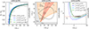 |
Fig. 1. Epicyclic frequencies and shape of tori. Left: epicyclic frequency ratio and shape of tori in the limit of β → 0. The dashed coloured vertical lines denote the locations of the ISCO calculated for different space-time parameters. The frequency-ratio values calculated for different space-time parameters at given radii are indicated by the coloured curves and labelled on the standard (left and bottom) axes. Several additional dashed ellipses, drawn for a non-rotating star (j = 0) and described by the upper and right axes, show the limiting cross-sections of slender tori located at a radius marked by the (common) lower axis. Middle: radial extension and shape of a torus with its centre located at radius r0 in the case of a non-rotating NS (j = 0). The dependence of the inner (rin) and outer (rout) torus radii on r0 is marked by orange (β = βcusp) and red (β = 0.2 βcusp) curves. Equipotential curves (black contours) are shown for two torus centre locations, r0 = 6.75 rG and r0 = 8 rG. The torus radial profile coordinates are identical to those on the bottom axes. Right: profiles of Keplerian specific angular momentum, l, corresponding to the same space-time parameters as in the left panel. The red horizontal line denotes a particular (chosen) value of l0. The shape of the cusp torus corresponding to this value of l0 and j = 0 is shown. As in the middle panel, the torus radial profile coordinates are identical to those on the bottom axis. The shape of equipotentials for the same value of l0 and the same space-time parameters is shown in Fig. 4. |
3.4. Explicit formulae in Hartle-Thorne space-time
The above general formulae describing tori are given in a self-consistent form, allowing for a straightforward description of tori. The implied explicit formulae describing the full solution for the accretion tori in the Hartle-Thorne space-time are rather long, and it would be challenging to fit them within this paper. Instead, we provide their complete version in a Wolfram Mathematica notebook3. This notebook contains functions for calculating important quantities of the metric and the shape of the equipotential surfaces for given parameters. The notebook includes a commentary to make it easier to read and use.
4. Solutions for astrophysically relevant space-time parameters
We illustrate the radial extension of tori around a non-rotating NS along with several equipotentials that determine the shape of possible tori in the middle panel of Fig. 1. In the case of a rotating NS, the space-time parameters will affect the shape of the solution, especially as it depends on the Keplerian angular momentum profile (as shown in the right panel of Fig. 1).
4.1. Impact of space-time parameters on the shape of tori
In the right panel of Fig. 1, we demonstrate the behaviour of the Keplerian angular momentum for chosen specific space-time parameters and compare it with the constant angular moment of the fluid (which is constant across the torus), and indicate the corresponding radial extension of the torus. In Fig. 2, we show how the radial extension of the tori depends on the location of the torus centre for fixed values of j and q/j2. We can see that the influence of NS rotation is greater for small values of q/j2 (left panel) and that, similarly to the case of the geodesic epicyclic frequency ratio, the behaviour corresponding to the moderate angular momentum along with the highest quadrupole moment considered, j = 0.3 and q = 10j2, is similar to the non-rotating case (right panel).
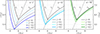 |
Fig. 2. Location of the cusp (rin) and the outer radius (rout) of the cusp tori for different values of r0 and space-time parameters, increasing in q/j2 from left to right. The curves denoting inner and outer radii merge in the limit of the slender cusp torus, i.e. when r0 = rISCO. The behaviour for the non-rotating case corresponds to the situation depicted along with several related details in the middle panel of Fig. 1. |
In Fig. 3, we present examples of the meridional cross-sections of the tori for several values of j and q/j2 in the case of a fixed torus centre position, r0. The left panel shows several examples of various cross-sections, and in the right panel special attention is given to the cusp tori cases.
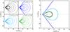 |
Fig. 3. Shape of tori calculated for a fixed torus centre, r0. Left: shape of tori calculated for the set of space-time parameters taken from Fig. 1 and a fixed value of r0 = 8rG (relevant values of l0 are determined by space-time parameters). The profiles are calculated for various increasing values of the thickness parameter, β. These values were chosen to smoothly cover the range from β = 0, corresponding to the case of a slender torus (central dot), through values corresponding to closed equipotential structures (i.e. tori), including the limiting case of cusp equipotentials (cusp torus), to the values corresponding to open equipotentials. Right: comparison of cusp torus configurations from the left panel. The black dot denotes the centre for all tori. |
We can see that, similar to the situation of slender tori determined by the ratio of the geodesic epicyclic frequencies depicted in the left panel of Fig. 1, the combined effect of the NS’s angular momentum and quadrupole moment on the non-slender torus shape does not imply any qualitative differences. Furthermore, the cusp tori corresponding to a moderate angular momentum (j = 0.3) and a high quadrupole moment(q = 10j2) are similar to the case of a non-rotating star. Indeed, the differences between the size of the cusp torus implied for j = 0 (black curve) and that for j = 0.3 and q = 10j2 (green curve) are minimal.
4.2. Coordinate-independent comparison
In Fig. 4, we present examples of the meridional cross-sections in the case of a fixed value of l0, which corresponds to the value marked in the right panel of Fig. 1. Even in this case, the same effect of compensation between the impacts of the angular momentum and quadrupole moment is clearly present. However, the differences between the size of the cusp torus implied for j = 0 (black curve) and that for j = 0.3 and q = 10j2 (green curve) are much more apparent.
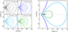 |
Fig. 4. Shape of tori calculated for a fixed value of the specific angular momentum, l0. Left: case for the same set of space-time parameters as in Fig. 1 and a fixed value of l0. The profiles are again determined for several values of the thickness parameter, β. Right: comparison of cusp torus configurations from the left panel. The dots denote the centres of each corresponding torus. |
By integrating Eq. (18), we can compare the sizes of the two cusp tori calculated for the same value of l0, denoted by the black and green contours in Fig. 4. We find that the torus calculated for the rotating oblate NS has a central density and mass several orders of magnitude higher than that calculated for a non-rotating NS.
5. Discussion and conclusions
We studied tori with thicknesses determined by the β parameter and, utilising the quadrupole parameter, found that the influences of the NS’s angular momentum and quadrupole moment were rather counterbalanced, which is to say that for a fixed radius of the centre, the solution for moderate angular momentum and a relatively large but still plausible quadrupole parameter was similar to the non-rotating case. This finding is in accordance with the results of several recent studies (Kluźniak & Rosińska 2013, 2014; Gondek-Rosińska et al. 2014) that explored the interplay between the relativistic frame-dragging effects given by the impact of angular momentum and the effects associated with the quadrupole moment that would also arise in Newtonian physics. Nevertheless, as we show in the comparison of the non-rotating and moderately rotating cases, cusp tori with the same specific angular momentum have very different sizes for different choices of space-time parameters.
5.1. Influence of the NS EoS
So far, we have focused on examining the effects of space-time parameters on accretion tori while considering a general range of these parameters associated with up-to-date models of NSs. However, a more thorough investigation of the implications given by the NS EoS is needed. In particular, the impact of the NS’s radius represents a significant challenge.
The inner edge of a torus with a given central radius and thickness parameter must be above the NS surface. Thus, the existence of a torus depends on the NS EoS, since it determines the NS radius assigned to a given mass and the rotation frequency. In this context, a necessary condition for the existence of cusp tori is that the NS surface is located below the ISCO, while the sufficient condition is that it is located below the IBO (e.g. Kozlowski et al. 1978; Abramowicz et al. 1978; Paczyński & Abramowicz 1982).
The radii of NSs given by various EoS are well determined by recently identified universal relations (Maselli et al. 2013; Urbanec et al. 2013; Yagi & Yunes 2013a,b; Pappas 2015; Reina et al. 2017). In Fig. 5, assuming these universal relations, we illustrate the size of two possible stars with the same mass and rotational frequency but a different NS angular momentum and quadrupole moment (namely, j = 0.205, q = 2.28j2 and j = 0.236, q = 2.84j2)4. For each star, we indicate the surface of the largest possible cusp torus that does not overlap with the NS surface as well as the sizes of a torus with various thicknesses, β. Clearly, while there is only a small difference in the NS size, the difference in the size of the tori is significant. Therefore, we expect the astrophysical applications of our results to be very sensitive to the NS EoS.
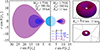 |
Fig. 5. Sizes of two NSs of the same mass and rotational frequency but different radii, calculated according to universal relations. The set of coloured tori illustrates the corresponding limits on the maximal size of the cusp tori that do not yet overlap with the star. The two NSs, along with their maximal cusp tori, are also shown in a 3D projection. |
5.2. Summary and overall implications
In this work, we have presented a solution of an equilibrium fluid torus in the Hartle-Thorne geometry that describes the space-time of a rotating NS. The solution includes the combined influence of the NS’s angular momentum and quadrupole moment on the underlying properties of tori, such as the position of the torus centre, its radial and vertical extent and overall size. We have paid special attention to the critically thick configurations – the cusp tori.
Given the above discussion, we can conclude that the quadrupole moment induced by the NS rotation should influence the observable spectral and temporal behaviour of tori. The underlying astrophysical applications, including the exploration of observational signatures of the NS EoS, need to focus on specific physical phenomena (such as the QPOs discussed in Paper II); we have provided publicly available tools for describing the tori.
Note the misprints in the original paper.
Here, M⊙ denotes the solar mass.
STL files with the 3D models of these two solutions can be downloaded from https://www.printables.com/model/794643-tori-around-neutron-stars
Acknowledgments
We thank Marek Abramowicz and Włodek Kluźniak for the valuable discussions. We also thank the reviewer for valuable comments and suggestions, which helped to significantly improve the paper. We acknowledge the Czech Science Foundation (GAČR) grant No. 21-06825X. The INTER-EXCELLENCE project No. LTT17003 is acknowledged by KK, and the INTER-EXCELLENCE project No. LTC18058 is acknowledged by MM and MU. We also thank the EU OPSRE project No. CZ.02.2.69/0.0/0.0/18_054/0014696 titled “Development of R&D capacities of the Silesian University in Opava”, and the PRODEX program of the European Space Agency (ref. 4000132152). VK acknowledges the Research Infrastructure LM2023047 of the Czech Ministry of Education, Youth and Sports. OS acknowledges funding by the Deutsche Forschungsgemeinschaft (DFG, German Research Foundation) under Germany’s Excellence Strategy – EXC 2094 – 390783311. We furthermore acknowledge the support provided by the internal grants of Silesian University, SGS/12, 13/2019, SGS/31/2023, SGS/25/2024, and SGF/1/2020, the latter of which has been carried out within the EU OPSRE project titled “Improving the quality of the internal grant scheme of the Silesian University in Opava”, reg. number: CZ.02.2.69/0.0/0.0/19_073/0016951.
References
- Abramowicz, M. A. 1971, Acta Astron., 21, 81 [NASA ADS] [Google Scholar]
- Abramowicz, M., Jaroszynski, M., & Sikora, M. 1978, A&A, 63, 221 [NASA ADS] [Google Scholar]
- Abramowicz, M. A., Almergren, G. J. E., Kluźniak, W., & Thampan, A. V. 2003, ArXiv e-prints [arXiv:gr-qc/0312070] [Google Scholar]
- Abramowicz, M. A., & Kato, S. 1989, ApJ, 336, 304 [NASA ADS] [CrossRef] [Google Scholar]
- Abramowicz, M. A., & Kluźniak, W. 2001, A&A, 374, L19 [NASA ADS] [CrossRef] [EDP Sciences] [Google Scholar]
- Abramowicz, M. A., & Kluźniak, W. 2005, Ap&SS, 300, 127 [NASA ADS] [CrossRef] [Google Scholar]
- Abramowicz, M. A., & Zurek, W. H. 1981, ApJ, 246, 314 [NASA ADS] [CrossRef] [Google Scholar]
- Abramowicz, M. A., Blaes, O. M., Horák, J., Kluźniak, W., & Rebusco, P. 2006, Class. Quant. Grav., 23, 1689 [NASA ADS] [CrossRef] [Google Scholar]
- Blaes, O. M. 1985, MNRAS, 216, 553 [CrossRef] [Google Scholar]
- Blaes, O. M., Arras, P., & Fragile, P. C. 2006, MNRAS, 369, 1235 [NASA ADS] [CrossRef] [Google Scholar]
- Bursa, M., Abramowicz, M. A., Karas, V., & Kluźniak, W. 2004, ApJ, 617, L45 [NASA ADS] [CrossRef] [Google Scholar]
- Cackett, E. M., Miller, J. M., Bhattacharyya, S., et al. 2008, ApJ, 674, 415 [NASA ADS] [CrossRef] [Google Scholar]
- Čadež, A., Calvani, M., & Kostić, U. 2008, A&A, 487, 527 [NASA ADS] [CrossRef] [EDP Sciences] [Google Scholar]
- de Avellar, M. G. B., Porth, O., Younsi, Z., & Rezzolla, L. 2018, MNRAS, 474, 3967 [NASA ADS] [CrossRef] [Google Scholar]
- Fabian, A. C., & Vaughan, S. 2003, MNRAS, 340, L28 [CrossRef] [Google Scholar]
- Fabian, A. C., Iwasawa, K., Reynolds, C. S., & Young, A. J. 2000, PASP, 112, 1145 [NASA ADS] [CrossRef] [Google Scholar]
- Fragile, P. C., Straub, O., & Blaes, O. 2016, MNRAS, 461, 1356 [NASA ADS] [CrossRef] [Google Scholar]
- Frank, J., King, A., & Raine, D. J. 2002, Accretion Power in Astrophysics, 3rd edn. (Cambridge: Cambridge University Press) [Google Scholar]
- Gimeno-Soler, S., & Font, J. A. 2017, A&A, 607, A68 [NASA ADS] [CrossRef] [EDP Sciences] [Google Scholar]
- Gondek-Rosińska, D., Kluźniak, W., Stergioulas, N., & Wiśniewicz, M. 2014, Phys. Rev. D, 89, 104001 [CrossRef] [Google Scholar]
- Hartle, J. B., & Thorne, K. S. 1968, ApJ, 153, 807 [NASA ADS] [CrossRef] [Google Scholar]
- Horák, J., Straub, O., Šrámková, E., Goluchová, K., & Török, G. 2017, RAGtime 17-19: Workshops on Black Holes and Neutron Stars, 47 [Google Scholar]
- Ingram, A., & Done, C. 2010, MNRAS, 405, 2447 [NASA ADS] [Google Scholar]
- Kato, S. 2001, PASJ, 53, 1 [NASA ADS] [CrossRef] [Google Scholar]
- Kato, S., Fukue, J., & Mineshige, S. 2008, Black-Hole Accretion Disks - Towards a New Paradigm (Kyoto University Press) [Google Scholar]
- Ketsaris, N. A., & Shakura, N. I. 1998, Astron. Astrophys. Trans., 15, 193 [NASA ADS] [CrossRef] [Google Scholar]
- Kluzniak, W., & Kita, D. 2000, ArXiv e-prints [arXiv:astro-ph/0006266] [Google Scholar]
- Kluźniak, W., & Rosińska, D. 2013, MNRAS, 434, 2825 [CrossRef] [Google Scholar]
- Kluźniak, W., & Rosińska, D. 2014, J. Phys. Conf. Ser., 496, 012016 [CrossRef] [Google Scholar]
- Kozlowski, M., Jaroszynski, M., & Abramowicz, M. A. 1978, A&A, 63, 209 [Google Scholar]
- Lančová, D., Abarca, D., Kluźniak, W., et al. 2019, ApJ, 884, L37 [CrossRef] [Google Scholar]
- Lattimer, J. M., & Prakash, M. 2001, ApJ, 550, 426 [NASA ADS] [CrossRef] [Google Scholar]
- Lattimer, J. M., & Prakash, M. 2007, Phys. Rep., 442, 109 [Google Scholar]
- Lewin, W., & van der Klis, M. 2010, Compact Stellar X-ray Sources (Cambridge: Cambridge University Press) [Google Scholar]
- Lo, K.-W., & Lin, L.-M. 2011, ApJ, 728, 12 [NASA ADS] [CrossRef] [Google Scholar]
- Maselli, A., Cardoso, V., Ferrari, V., Gualtieri, L., & Pani, P. 2013, Phys. Rev. D, 88, 023007 [NASA ADS] [CrossRef] [Google Scholar]
- Matuszková, M., Török, G., Klimovičová, K., et al. 2024, A&A, 691, A168 [NASA ADS] [CrossRef] [EDP Sciences] [Google Scholar]
- McClintock, J. E., & Remillard, R. A. 2006, Compact Stellar X-ray Sources (Cambridge: Cambridge University Press), 39 157 [Google Scholar]
- McClintock, J. E., Narayan, R., & Shafee, R. 2011, in Black Holes, eds. M. Livio, & A. M. Koekemoer (Cambridge: Cambridge University Press), 252 [CrossRef] [Google Scholar]
- Miller, J. M., Zoghbi, A., Raymond, J., et al. 2020, ApJ, 904, 30 [Google Scholar]
- Mishra, B., Vincent, F. H., Manousakis, A., et al. 2017, MNRAS, 467, 4036 [CrossRef] [Google Scholar]
- Paczyński, B., & Abramowicz, M. A. 1982, ApJ, 253, 897 [NASA ADS] [CrossRef] [Google Scholar]
- Papaloizou, J. C. B., & Pringle, J. E. 1984, MNRAS, 208, 721 [NASA ADS] [CrossRef] [Google Scholar]
- Pappas, G. 2015, MNRAS, 454, 4066 [NASA ADS] [CrossRef] [Google Scholar]
- Piraino, S., Santangelo, A., Kaaret, P., et al. 2012, A&A, 542, L27 [NASA ADS] [CrossRef] [EDP Sciences] [Google Scholar]
- Qian, L., Abramowicz, M. A., Fragile, P. C., et al. 2009, A&A, 498, 471 [NASA ADS] [CrossRef] [EDP Sciences] [Google Scholar]
- Reina, B., Sanchis-Gual, N., Vera, R., & Font, J. A. 2017, MNRAS, 470, L54 [CrossRef] [Google Scholar]
- Reynolds, C. S., & Fabian, A. C. 2008, ApJ, 675, 1048 [NASA ADS] [CrossRef] [Google Scholar]
- Rezzolla, L., Yoshida, S., Maccarone, T. J., & Zanotti, O. 2003a, MNRAS, 344, L37 [CrossRef] [Google Scholar]
- Rezzolla, L., Yoshida, S., & Zanotti, O. 2003b, MNRAS, 344, 978 [NASA ADS] [CrossRef] [Google Scholar]
- Riaz, S., Ayzenberg, D., Bambi, C., & Nampalliwar, S. 2020a, ApJ, 895, 61 [NASA ADS] [CrossRef] [Google Scholar]
- Riaz, S., Ayzenberg, D., Bambi, C., & Nampalliwar, S. 2020b, MNRAS, 491, 417 [NASA ADS] [CrossRef] [Google Scholar]
- Shafee, R., Narayan, R., & McClintock, J. E. 2008, ApJ, 676, 549 [NASA ADS] [CrossRef] [Google Scholar]
- Steiner, J. F., McClintock, J. E., Remillard, R. A., Narayan, R., & Gou, L. 2009, ApJ, 701, L83 [NASA ADS] [CrossRef] [Google Scholar]
- Steiner, J. F., McClintock, J. E., Remillard, R. A., et al. 2010, ApJ, 718, L117 [Google Scholar]
- Stella, L., & Vietri, M. 1998, in 19th Texas Symposium on Relativistic Astrophysics and Cosmology, eds. J. Paul, T. Montmerle, & E. Aubourg [Google Scholar]
- Strohmayer, T. E., Zhang, W., Swank, J. H., et al. 1996, ApJ, 469, L9 [Google Scholar]
- Török, G., Abramowicz, M. A., Kluźniak, W., & Stuchlík, Z. 2005, A&A, 436, 1 [NASA ADS] [CrossRef] [EDP Sciences] [Google Scholar]
- Urbancová, G., Urbanec, M., Török, G., et al. 2019, ApJ, 877, 66 [CrossRef] [Google Scholar]
- Urbanec, M., Miller, J. C., & Stuchlík, Z. 2013, MNRAS, 433, 1903 [CrossRef] [Google Scholar]
- Wagoner, R. V. 1999, Phys. Rep., 311, 259 [NASA ADS] [CrossRef] [Google Scholar]
- Yagi, K., & Yunes, N. 2013a, Phys. Rev. D, 88, 023009 [CrossRef] [Google Scholar]
- Yagi, K., & Yunes, N. 2013b, Science, 341, 365 [NASA ADS] [CrossRef] [Google Scholar]
All Figures
|
Fig. 1. Epicyclic frequencies and shape of tori. Left: epicyclic frequency ratio and shape of tori in the limit of β → 0. The dashed coloured vertical lines denote the locations of the ISCO calculated for different space-time parameters. The frequency-ratio values calculated for different space-time parameters at given radii are indicated by the coloured curves and labelled on the standard (left and bottom) axes. Several additional dashed ellipses, drawn for a non-rotating star (j = 0) and described by the upper and right axes, show the limiting cross-sections of slender tori located at a radius marked by the (common) lower axis. Middle: radial extension and shape of a torus with its centre located at radius r0 in the case of a non-rotating NS (j = 0). The dependence of the inner (rin) and outer (rout) torus radii on r0 is marked by orange (β = βcusp) and red (β = 0.2 βcusp) curves. Equipotential curves (black contours) are shown for two torus centre locations, r0 = 6.75 rG and r0 = 8 rG. The torus radial profile coordinates are identical to those on the bottom axes. Right: profiles of Keplerian specific angular momentum, l, corresponding to the same space-time parameters as in the left panel. The red horizontal line denotes a particular (chosen) value of l0. The shape of the cusp torus corresponding to this value of l0 and j = 0 is shown. As in the middle panel, the torus radial profile coordinates are identical to those on the bottom axis. The shape of equipotentials for the same value of l0 and the same space-time parameters is shown in Fig. 4. |
| In the text | |
|
Fig. 2. Location of the cusp (rin) and the outer radius (rout) of the cusp tori for different values of r0 and space-time parameters, increasing in q/j2 from left to right. The curves denoting inner and outer radii merge in the limit of the slender cusp torus, i.e. when r0 = rISCO. The behaviour for the non-rotating case corresponds to the situation depicted along with several related details in the middle panel of Fig. 1. |
| In the text | |
|
Fig. 3. Shape of tori calculated for a fixed torus centre, r0. Left: shape of tori calculated for the set of space-time parameters taken from Fig. 1 and a fixed value of r0 = 8rG (relevant values of l0 are determined by space-time parameters). The profiles are calculated for various increasing values of the thickness parameter, β. These values were chosen to smoothly cover the range from β = 0, corresponding to the case of a slender torus (central dot), through values corresponding to closed equipotential structures (i.e. tori), including the limiting case of cusp equipotentials (cusp torus), to the values corresponding to open equipotentials. Right: comparison of cusp torus configurations from the left panel. The black dot denotes the centre for all tori. |
| In the text | |
|
Fig. 4. Shape of tori calculated for a fixed value of the specific angular momentum, l0. Left: case for the same set of space-time parameters as in Fig. 1 and a fixed value of l0. The profiles are again determined for several values of the thickness parameter, β. Right: comparison of cusp torus configurations from the left panel. The dots denote the centres of each corresponding torus. |
| In the text | |
|
Fig. 5. Sizes of two NSs of the same mass and rotational frequency but different radii, calculated according to universal relations. The set of coloured tori illustrates the corresponding limits on the maximal size of the cusp tori that do not yet overlap with the star. The two NSs, along with their maximal cusp tori, are also shown in a 3D projection. |
| In the text | |
Current usage metrics show cumulative count of Article Views (full-text article views including HTML views, PDF and ePub downloads, according to the available data) and Abstracts Views on Vision4Press platform.
Data correspond to usage on the plateform after 2015. The current usage metrics is available 48-96 hours after online publication and is updated daily on week days.
Initial download of the metrics may take a while.