| Issue |
A&A
Volume 638, June 2020
|
|
|---|---|---|
| Article Number | A138 | |
| Number of page(s) | 15 | |
| Section | Cosmology (including clusters of galaxies) | |
| DOI | https://doi.org/10.1051/0004-6361/201936437 | |
| Published online | 26 June 2020 | |
Implications of the mild gas motion found with Hitomi in the core of the Perseus cluster
1
RIKEN High Energy Astrophysics Laboratory, 2-1 Hirosawa, Wako, Saitama 351-0198, Japan
2
SRON Netherlands Institute for Space Research, Sorbonnelaan 2, 3584 CA Utrecht, The Netherlands
e-mail: This email address is being protected from spambots. You need JavaScript enabled to view it.
3
Department of Physics, Graduate School of Science, The University of Tokyo, 7-3-1 Hongo, Bunkyo-ku, Tokyo 113-0033, Japan
4
Kavli IPMU, The University of Tokyo, 5-1-1 Kashiwa-no-ha, Kashiwa 277-8535 Chiba, Japan
5
Department of Physics, Graduate School of Science, Chiba University, 1-33 Yayoi-cho, Inage-ku, Chiba 263-8522, Japan
6
Kobayashi-Maskawa Institute for the Origin of Particles and the Universe, Nagoya University, Furo-cho, Chikusa-ku, Nagoya, Aichi 464-8601, Japan
7
Department of Astronomy, Graduate School of Science, The University of Tokyo, 7-3-1 Hongo, Bunkyo-ku, Tokyo 113-0033, Japan
8
Research Center for the Early Universe, Graduate School of Science, The University of Tokyo, 7-3-1 Hongo, Bunkyo-ku, Tokyo 113-0033, Japan
9
Department of Physics, Nara National College of Technology, Yamatokohriyama, Nara 639-1080, Japan
10
Astronomical Institute, Tohoku University, Aramaki, Aoba-ku, Sendai 980-8578, Japan
11
School of Physics and Astronomy, Shanghai Jiao Tong University, 800 Dongchuan Road, Shanghai 200240, PR China
12
Tsung-Dao Lee Institute, Shanghai Jiao Tong University, 800 Dongchuan Road, Shanghai 200240, PR China
13
IFSA Collaborative Innovation Center, Shanghai Jiao Tong University, 800 Dongchuan Road, Shanghai 200240, PR China
14
Tsukuba Space Center (TKSC), Japan Aerospace Exploration Agency (JAXA), 2-1-1 Sengen, Tsukuba, Ibaraki 305-8505, Japan
Received:
2
August
2019
Accepted:
4
May
2020
Abstract
Based mainly on X-ray observations, we study the interactions between the intracluster medium (ICM) in clusters of galaxies and their member galaxies. Through (magneto)hydrodynamic and gravitational channels, moving galaxies are expected to drag the ICM around them, and then transfer some fraction of their dynamical energies on cosmological timescales to the ICM. This hypothesis is in line with several observations, including the possible cosmological infall of galaxies toward the cluster center, found over redshifts of z ∼ 1 to z ∼ 0. Further assuming that the energy lost by these galaxies is first converted into ICM turbulence and then dissipated, this picture can explain the subsonic and uniform ICM turbulence, measured with Hitomi in the core region of the Perseus cluster. The scenario may also explain several other unanswered problems regarding clusters of galaxies, such as what prevents the ICM from underoing the expected radiative cooling, how the various mass components in nearby clusters have attained different radial distributions, and how a thermal stability is realized between hot and cool ICM components that co-exist around cD galaxies. This view is also considered to pertain to the general scenario of galaxy evolution, including their environmental effects.
Key words: galaxies: clusters: intracluster medium / galaxies: interactions / turbulence / X-rays: galaxies: clusters
© ESO 2020
1. Introduction
The most dominant observed form of cosmic baryons is found as intracluster medium (ICM), i.e., the X-ray emitting hot plasmas gravitationally confined in individual clusters of galaxies. The ICM is still subject to a series of unsolved puzzles, including the balance between cooling and heating. Since the radiative cooling time of ICM at the center of rich clusters is significantly shorter than the Hubble time tH, these plasmas were thought to cool and gradually lose their pressure. This creates inward plasma motion called cooling flows (CFs), which further increase the density of the ICM in the central region of the cluster and enhance its radiative cooling. The operation of this feedback was apparently supported by early imaging spectroscopic observations of a number of clusters in soft X-rays. To be specific, clusters that host cD galaxies, or cD clusters, ubiquitously show a series of characteristic phenomena within ∼100 kpc of the cD galaxy, including an inward decrease in the ICM temperature and a strongly peaked brightness distribution therein (Fabian 1994).
As X-ray imaging spectroscopy became available in a broader energy band (up to 10 keV) with better energy resolution, it was confirmed that the cluster core regions indeed host cooler X-ray emission, hereafter called the central cool component (CCC). However, essentially in all galaxy clusters and groups, plasma components with temperatures below ∼0.5 keV have been revealed to be much less than predicted by the CF scenario. This puzzling discovery, first made with ASCA (Ikebe et al. 1999; Makishima et al. 2001), was reinforced through observations with XMM-Newton (Peterson et al. 2001; Xu et al. 2002), Chandra (Fabian et al. 2001), and Suzaku (Gu et al. 2012). As a result, the nomenclature of cool-core clusters was adopted instead of CF clusters. Apparently, the ICM is somehow heated against radiative cooling, so that the expected CFs are suppressed or mitigated.
Among several candidate mechanisms proposed to explain ICM heating, the most popular is the so-called active galactic nucleus (AGN) feedback scenario (Churazov et al. 2001; Fabian et al. 2000; McNamara & Nulsen 2007; Fabian 2012). According to this conjecture, the AGN of the central (usually cD) galaxy in a cluster operates in a kinetic/radio mode, by accreting the surrounding cold/hot matter at a sub-Eddington rate, and releasing most of the gravitational energy into radio jets or inflating bubbles instead of radiation. The heating is considered to balance the radiative ICM cooling through an inherent negative feedback mechanism; enhanced cooling increases the ICM density surrounding the central black hole, making the AGN more active, thus providing a higher heating luminosity to be deposited on the ICM. Although the scenario is presented with many theoretical variants, generally highly collimated AGN jets are assumed to be transporting the energy from the black hole to a very limited fraction of the ICM volume (i.e., not volume-filling). Therefore, the scenario requires another mechanism to efficiently redistribute the deposited energy over the cluster core volume. One of the promising candidates was propagation of strong turbulence created by the AGN jets (Enßlin & Vogt 2006; Chandran & Rasera 2007; Scannapieco & Brüggen 2008; Kunz et al. 2011). Then, the heat from the turbulence dissipation would spread over the cool core within the cooling timescale, so as to offset the CFs.
In its brief lifetime, the Hitomi Observatory (Takahashi et al. 2014) obtained a set of X-ray spectra from central regions of the Perseus cluster of galaxies, with the Soft X-ray Spectrometer (SXS) which is a nondispersive detector with a superb energy resolution. Using the Fe-K line widths measured with the SXS, the turbulence velocity dispersion was found to be ∼164 km s−1 in a region 30−60 kpc from the central nucleus, and the shear in the bulk motion was found to be ∼150 km s−1 across the central 60 kpc region (Hitomi Collaboration 2016). Further analysis of the SXS data revealed that the velocity dispersion is relatively uniform within the central 100 kpc, except for the innermost core (r < 20 kpc) and the vicinity of an AGN cavity, where mild increases were observed (Hitomi Collaboration 2018a). The average energy density contained in the turbulence is estimated to be ∼4% of the total ICM thermal energy density.
These Hitomi results have brought some difficulties into the ICM heating mechanisms that invoke AGN activity and consequent turbulence. First, owing to the low energy density, the turbulence would only be able to sustain the X-ray emission for a very short time, 8 × 10⁷ years, or 0.006 tH (Hitomi Collaboration 2016). Second, to maintain a stable balance between cooling and heating, the turbulence must be replenished on the same timescale, but this is not necessarily obvious. Furthermore, in 8 × 10⁷ years, such a low-speed (∼164 km s−1) turbulence would propagate from the excitation sources only over ∼13 kpc, which is far too insufficient to heat the entire cool core (Fabian et al. 2017). In short, given the Hitomi results, it would be difficult to heat the ICM in the cool core of the Perseus cluster globally for a sufficiently long time, if we only consider the random gas motions driven by the AGN jets and bubbles.
The above evaluations all assumed that the X-ray emission from the cluster core, contributing a large fraction (∼80%) of the total X-ray luminosity, must be sustained by the turbulence energy of the core-region ICM, which carries a small fraction (∼10%) of the overall ICM mass. Therefore, the problem could be mitigated by assuming significant energy transport in other forms, for example, heat conduction from outer regions to the core (Voigt & Fabian 2004), mixing of the hot injected gas with the cooling ICM (Hillel & Soker 2017, 2019), or sound waves from the AGN (Fabian et al. 2017; Zweibel et al. 2018; Bambic et al. 2018). Deep X-ray imaging of the Perseus cluster hints at the latter, if the surface brightness fluctuations found in the core are indeed sound waves from the bubbles (Fabian et al. 2003, 2006; Sanders & Fabian 2007). What still remains controversial is whether the sound waves can be dissipated just as they propagate across the cool core region (Ruszkowski et al. 2004; Fujita & Suzuki 2005).
Another possible way around these difficulties was proposed by Lau et al. (2017) based on numerical simulations, introducing a fair amount of changes to the AGN feedback model. These authors assume a series of frequent small outbursts from the central AGN, instead of a few powerful outbursts. The induced turbulence field would then be low and flat because the input kinetic energy is low and steady. However, Lau et al. still need to call for accretion of member galaxies and subclusters to explain the mild line-of-sight velocity gradient observed with Hitomi because such a gentle AGN feedback would be too uniform to explain the observed bulk velocity gradient. A similar conclusion was reached by Bourne & Sijacki (2017) based on a different simulation.
Motivated by these difficulties, in the present work we focus on a relatively unexplored aspect of clusters of galaxies: interactions between the two major baryonic components, namely, the moving member galaxies and the ICM. As briefly summarized in Sect. 2, this idea was first proposed by Makishima et al. (2001, hereafter Paper I) based on ASCA observations and incorporating some semiquantitative evaluations. Since then, the view has been reinforced by a series of data-oriented studies (see Sect. 3) with XMM-Newton (Takahashi et al. 2009; Kawaharada et al. 2009), Chandra, and Suzaku (Gu et al. 2012), as well as by extensive X-ray versus optical comparisons of clusters at various redshifts (Gu et al. 2013a, 2016). The emerging scenario can potentially solve some of the issues with the ICM, including its temperature structures, the metal distributions in it, and the suppression of CFs.
Our scenario also has rich implications for ICM turbulence. The assumed physical interactions between the galaxies and ICM and the consequent gravitational perturbations, create magnetohydrodynamical (MHD) turbulence in situ throughout the cluster core. The turbulence is naturally expected to be volume-filling thanks to the high galaxy density in the core region (one per 50−100 kpc3; Budzynski et al. 2012; Gu et al. 2016), and must be subsonic because the galaxies are moving through the ICM with trans-sonic velocities. A numerical simulation by Ruszkowski & Oh (2011) based on a similar scenario predicts σ = 150−250 km s−1, in good agreement with the Hitomi measurements. In the present paper, we discuss how this scenario has been reinforced by the Hitomi results.
2. Review of the proposed scenario
In this section, we briefly review our interpretations of the physics in central regions of cD clusters. The first set of assumptions presented in Sect. 2.1 deal with spatial magnetic and temperature structures of the ICM in a static sense, while the second set in Sect. 2.2 describe dynamics and cosmological evolution of the physical conditions therein.
2.1. Basic assumptions (1): Static aspects
In order to describe static magnetic structures of the ICM in central regions of cD clusters, we start from a generally accepted view, which is that the ICM is hydrostatically confined by gravity and is magnetized to β ∼ 30−300, where β is the thermal plasma pressure relative to the magnetic pressure. That is, the magnetic energy density amounts to a fraction of percent to a few percent of the average thermal energy density (Böhringer et al. 2016). In addition, we adopt the following first set of assumptions (Paper I; Takahashi et al. 2009; Gu et al. 2012). The overall configuration is referred to as “cD corona” picture.
S1 The ICM in the cluster core region has relatively well-ordered magnetic structures because the cD galaxy is approximately standstill with respect to the ICM.
S2 The magnetic field lines (MFLs) in the cluster core region are classified into two types: closed loops with both ends anchored to the cD galaxy and open loops with at most one end attached to the galaxy.
S3 The open-MFL regions are filled with the hot isothermal ICM, whereas the closed MFLs confine a cooler and more metal-rich plasma, identified with the CCC, to form a magnetosphere. The two plasma phases are in an approximate pressure equilibrium.
Of these assumptions, S1 is a natural consequence of the unique location of a cD galaxy, that is, the center of the gravitational potential. The second assumption is just a basic and general classification of MFLs, as observed in solar coronae and interplanetary space. A related discussion, on a possibility of tangled MFLs, is presented in Sect. 4.1.2. The assumption S3 is also a prediction by plasma physics. The open-MFL regions, connected to the outer ICM, is brought into a global isothermality on a timescale of ∼108 yr by the high thermal conductivity along the MFLs. In contrast, the CCC can have a different temperature and metallicity because the particle and heat transport is strongly suppressed across the MFLs. The CCC plasma is considered to partially originate from the cD galaxy.
The cD corona model (S1−S3) may naturally explain several characteristic features seen in the cluster central regions. First, filamentary structures in the optical line emission have been observed around many cD galaxies on scales of ∼10−100 kpc (Conselice et al. 2001; Crawford et al. 2005; McDonald et al. 2012, 2015). Considering that these structures are likely to trace the closed MFLs, the assumed configuration is consistent with the observed coexistence of different gaseous components in the core region: some are cool and dense while others are hot and tenuous.
Second, the ICM around cD galaxies indeed shows stratified temperature structures as in S3. The X-ray spectra from these regions require a two-phase (2P) modeling, employing two temperatures that represent the hot ICM and the CCC (Ikebe et al. 1999; Tamura et al. 2003; Takahashi et al. 2009; Gu et al. 2012; Walker et al. 2015; de Plaa et al. 2017). In contrast, those from outer regions can be described by a single-phase (1P) modeling. The 2P condition cannot be an artifact arising from the projection effects because Takahashi et al. (2009) and Gu et al. (2012) showed, through a careful deprojection procedure, that the CCC and the hot phase spatially coexist in the three-dimensional core region of cool-core clusters. Since the hot phase is often two to three times hotter than the CCC, the CCC must be confined by MFLs and thermally shielded from the hot phase. The cool-phase gas is free to move along the closed MFLs, so that it is approximately in a pressure equilibrium with the hot phase.
Finally, the structure of intracluster MFLs (S1) can be directly probed through Faraday rotation measurements of radio signals from background sources or cluster member galaxies. These measurements of the cluster central regions reveal coherence scales of 2−25 kpc (Taylor & Perley 1993; Feretti et al. 1999; Govoni et al. 2001; Eilek & Owen 2002; Clarke 2004), indicating that the MFLs may also have a spatial order on such scales, instead of being completely tangled.
2.2. Basic assumptions (2): Dynamical aspects
The first set of assumptions (S1−S3) above are complemented by the following second set of assumptions (Paper I; Takahashi et al. 2009; Gu et al. 2012, 2013a, 2016), which describe dynamical and evolutionary aspects of the problem.
D1 Non-cD member galaxies, moving through the ICM at its trans-sonic velocities, interact with the ICM, and transfer to it some fraction of their dynamical energies on a cosmological timescale.
D2 The member galaxies, thus losing the energy, gradually fall toward the center of the potential, while supplying metal-enriched interstellar medium (ISM) to the ICM.
D3 The energy deposited onto the ICM first takes the form of MHD turbulence, which is then thermalized to provide a heating luminosity of ∼1044 erg s−1, which is needed to balance the radiative cooling, particularly in the CCC.
D4 Throughout the heating process, the two plasma phases are kept in a pressure equilibrium and are thermally stablized by the Rosner-Tucker-Vaiana (RTV; Rosner et al. 1978) mechanism, which operates in solar coronae.
Of these assumptions, probably the least accepted idea would be D1 because galaxies are generally believed to swim freely through the ICM with insignificant energy dissipation. However, as explained in Sect. 3.1 and further in Sect. 5.1, this popular belief is not necessarily warranted. Furthermore, the assumption D2, which is an immediate consequence of D1, is now supported by indirect (Sect. 3.2.1) and direct (Sect. 3.2.2) observations, as well as numerical studies.
We assign the entire Sect. 4 to the discussion concerning D3 because it is most relevant to the Hitomi results. Finally, D4 may appear too specific. However, as described in Sect. 5.2, D4 is a direct consequence of the cD corona configuration, and is an essential ingredient of our overall scenario because it provides a very natural way to thermally stabilize the CCC.
3. Scenario of galaxy-ICM interaction
Addressing the assumptions in the dynamical aspects (Sect. 2.2) is in essence to find answers to the following three key questions: (1) we ask whether the ICM interact with the member galaxies and contribute significantly to their evolution; (2) whether the dynamics of member galaxies are also affected appreciably by the presence of the ICM; and (3) conversely, whether the moving galaxies at all influence the thermodynamical evolution of the ICM. We examine these issues below.
3.1. Evidence for the interaction: Ram pressure stripping and environmental effects
First, we review observational evidence for the galaxy-ICM interaction and point out its important role in the evolution of member galaxies. These results altogether answer the first key issue raised above affirmatively.
As suggested in the early work by Gunn & Gott (1972) and confirmed by observations (van Gorkom 2004, and references therein), any gaseous interstellar material in a galaxy, collectively called the ISM, would feel the ram pressure of the ICM as the galaxy moves through the cluster. When the ram pressure exceeds the gravitational restoring force, the ISM in outer galaxy disks is stripped off, to form a tail in the trailing wake of the galaxy. While the loss of ISM suppresses the star formation in outer regions of the galaxy, the ram pressure at the same time compresses the ISM in the central regions and tails, to enhance the star formation therein (Fujita & Nagashima 1999; van Gorkom 2004; Vollmer et al. 2006). The efficient removal of the metal-rich ISM is in line with the fact that the ICM contains a large amount of metals, comparable to those contained in stars, and the ICM metallicity is very uniform up to the periphery (described later).
Some statistical studies indicate that the ram pressure effects are ubiquitous. An Hα and R band imaging of 55 spiral galaxies in the Virgo cluster showed truncated star-forming disks in 52% of the sample galaxies, which are likely the product of galaxy-ICM interaction (Koopmann & Kenney 1998, 2004; Abadi et al. 1999). Although the so-called galaxy harassment (Moore et al. 1996) could also be contributing, Couch et al. (1998) used Hubble Space Telescope data of three clusters to argue that the star formation is more efficiently truncated by ram pressure than by harassment. The observed optical and H I properties motivated many authors (e.g., Bösch et al. 2013; Rodríguez Del Pino et al. 2014) to propose an evolutionary route of galaxies, beginning with field-like spirals and transforming, via long-term ram pressure stripping and passive fading, into proto-S0 galaxies.
The statistical studies mentioned above can be generalized into the well-known concept of “environmental effects”. It is long known that, at low redshifts, the galaxies in crowded environments predominantly have early-type morphology (Oemler 1974; Dressler 1980), red color (Pimbblet et al. 2002; Balogh et al. 2004), and suppressed star formation rates (Balogh et al. 1998; Goto et al. 2003). Although the main population of member galaxies in local clusters is thus red and inactive, the presence of blue star-forming galaxies in rich clusters at z ∼ 0.5 has been known since the early work by Butcher & Oemler (1984). These two environmental effects, one spatial and the other temporal, can be naturally and consistently explained by assuming that the presence of the ICM and neighboring galaxies accelerates the galaxy evolution, including the morphology and color changes and the rapid decline in the star formation rate.
3.2. Evidence of galaxy infall
We have so far answered affirmatively to the first key issue presented at the beginning of this section; the ICM indeed interacts with the moving galaxies and is likely to accelerate their evolution. Next we address the key issue (2), whether the interaction also affects the dynamics of galaxies, and causes the galaxies to slow down and gradually fall toward the cluster center. Below, direct observations of possible galaxy infall on cosmological timescales (e.g., Gu et al. 2013a, 2016; Sect. 3.2.2) are augmented by several pieces of indirect observational evidence from different aspects (Sect. 3.2.1).
3.2.1. Radial distributions of baryons and metallicity therein
In nearby clusters of galaxies, the three major mass components are well known to show systematically different radial profiles; relative to dark matter (DM), the ICM is slightly more extended, whereas member galaxies are much more concentrated (Bahcall 1999). Figure 1 (left) directly compares the radial distributions of the galaxies and ICM, both averaged over 119 clusters at z < 0.08. Within a radius of ∼R500 beyond which the measurements become less accurate, the ICM shows a flatter radial distribution than the galaxy component. To quantify the difference, we introduce a quantity called the galaxy light-to-ICM mass ratio (GLIMR; Gu et al. 2013a), which is the ratio of the circularly (two-dimensionally) integrated galaxy light divided by the ICM mass integrated similarly. Then, in nearby clusters, GLIMR typically decreases by a factor of 2 from r = 0.2 R500 to r = 0.5 R500 (Gu et al. 2013a, 2016). One possible explanation of the GLIMR gradient would be provided by our assumptions D1 and D2, which predict that galaxies should gradually sink to the center by losing their dynamical energies to the environment, and the energy deposited to the ICM makes it expand relative to the DM. If it works continuously, the GLIMR profile is steepened over time, which is in qualitative agreement with our scenario.
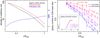 |
Fig. 1. Left panel: projected radial density profiles (left ordinate) of the galaxy surface number (black) and the ICM (red) in nearby (z ≤ 0.08) clusters, normalized at a radius of 0.05 R500. Both data are taken from the sample of Gu et al. (2016). The ICM to galaxy density ratio is plotted in blue (right ordinate). Right panel: observed GNIMR profiles averaged over clusters in different redshift bins. This plot shows a combination of two samples, 34 clusters (z = 0.1−0.9) from Gu et al. (2013a, open symbols), and 340 clusters (z = 0−0.5) from Gu et al. (2016, filled symbols). Error bars are at the 1σ level. The r-band luminosity functions of the identified member galaxies from the 340 cluster sample in different redshift bins are shown in the inset. |
Since metals in the ICM must have originated from galaxies, and can serve as a tracer of the past galaxy distributions, their large-scale spatial behavior helps us to understand the present-day mass distributions. At this point, we should consider two important observational facts. One is the result obtained with the Suzaku XIS, that the ICM metallicity in the outskirts (with a two-dimensional radius r > 1 Mpc) of several clusters are spatially fairly constant at ∼0.3 solar (Werner et al. 2013). The observed constant metallicity at larger radii is usually taken for evidence that the metal enrichment of ICM took place very early, at redshifts of z = 2−3 before the cluster formation, via strong galaxy winds and/or AGN outflows (Fujita et al. 2008; Werner et al. 2013). In this case, an implicit assumption is that stars at these early epochs distributed out to very large radii and provided the initial metals to the ICM therein. However, as indicated by the GLIMR behavior, the present-day clusters do not harbor, at their peripheries, the corresponding population of galaxies. Therefore, simply invoking the “early metal enrichment” view alone would not easily bring into agreement the overall observational facts quoted so far.
As a natural way to bring the early ICM enrichment scenario into agreement with the present-day GLIMR profiles, we assume that the metal-supplying stars formed galaxies in the peripheral regions, which then gradually fell toward smaller radii, as in our assumption D2. At the beginning of this process, the metals were transported to the intracluster space presumably via galactic winds (Fujita et al. 2008), but as the galaxies moved to regions of higher ICM densities, for example, ≲1 Mpc, the role of ram pressure stripping of metal-enriched ISM is considered to have become gradually more important (Fujita & Nagashima 1999). This agrees with the very mild inward increase of the ICM metallicity, observed on intermediate radii from ≲1 Mpc down to ∼100 kpc (Matsushita et al. 2003; Johnson et al. 2011; Mernier et al. 2017).
The other observational fact to be considered is the behavior of a quantity called metal mass-to-light ratio (MMLR), that is, the circularly integrated metal mass in the ICM divided by the galaxy light integrated in the same way. In many nearby clusters and groups, MMLR has been observed to increase, from the center to ∼100 kpc, by nearly two orders of magnitude (Sato et al. 2007, 2009a,b; Kawaharada et al. 2009; Sasaki et al. 2014). This outward MMLR increase must continue beyond 100 kpc out to larger radii because we have MMLR ∝ metallicity/GLIMR, where the metallicity is rather constant to the periphery (the first fact), and GLIMR decreases outward (Sect. 3.2.2). In short, the present-day galaxies are more concentrated relative to not only the ICM, but also the metals in it. This can also be explained in a natural way by our assumption D2.
3.2.2. Direct observations of galaxy infall
Although the spatial distributions of the different components in nearby clusters have been shown (Sect. 3.2.1) to support to our dynamical assumptions, a more direct confirmation of the scenario was awaiting for a comparison of distant clusters with their nearby counterparts. This has finally been carried out successfully by Gu et al. (2013a); the authors studied a carefully selected sample of 34 clusters in a redshift range of z = 0.1−0.9, both in the optical and X-ray frequencies, to compare the optical and X-ray angular extents of individual clusters in the sample. All the selected clusters have relaxed X-ray morphologies and harbor cD galaxies at their centers. Since the utilized optical data were photometric rather than spectroscopic, the galaxy membership in each cluster was determined using photometric redshifts, supplemented by an offset pointing. Then, as reproduced in Fig. 1 (right) with open symbols, the GLIMR profiles of these clusters were found to be originally flat at z ∼ 0.9, and were evolving to become steeper as the redshift decreases. We believe that this provides one of the fundamental evolutionary effects ever observed from clusters of galaxies.
Utilizing a much larger sample consisting of 340 SDSS clusters, though with a shallower redshift coverage of z = 0.0−0.5, Gu et al. (2016) carried out a more sensitive follow-up study of the galaxy-to-ICM evolution. This time, a fraction of the optical data were spectroscopic, and a quantity galaxy number-to-ISM mass ratio (GNIMR) was used instead of GLIMR. Then, as shown in Fig. 1 (right) with filled symbols, the X-ray versus optical comparison again revealed a clear relative evolution, which agrees quantitatively with the first result by Gu et al. (2013a). In addition, Gu et al. (2016) found that the galaxies became radially more concentrated with respect to the DM component as well. At the same time, the luminosity functions of the member galaxies used by Gu et al. (2016) were confirmed approximately the same over the relevant redshift range (inset to Fig. 1 right). Therefore, the enhancement of galaxies in the cluster center toward z ∼ 0 cannot be ascribed to a recent galaxy/star formation. Instead, the galaxies from the cluster periphery likely have moved inward, with respect to both the ICM and DM, on a timescale of ≥6 Gyr.
The dynamical evolution of member galaxies in clusters has also been investigated using numerical simulations, where the galaxy-scale processes such as ram pressure stripping have been reproduced utilizing progressively finer spatial grids (∼kpc or less). A recent hydrodynamical work by Armitage et al. (2018) explored the evolution of velocity dispersion of member galaxies as a function of time spent inside the cluster. As shown in their Fig. 8, the member galaxies are indeed found to be slowing down after their first passage through the cluster core. If normalized to the velocity of dark matter, the velocities of member galaxies decrease by ∼20% after spending 10 Gyr in the cluster. Naturally these galaxies fall toward the cluster center as they become slower than the ambient dark matter particles. Although these authors mainly considered gravitational dynamical friction, the slowdown of their galaxies was found to be little dependent on the total galaxy mass, contrary to what is expected from the pure gravitational interaction (Eq. (8)). Therefore, we infer that other forms of galaxy-cluster interaction, such as the ram pressure process, are likely to be contributing to the slowdown of their model galaxies. Similar galaxy slowdown and infall have been observed in other hydrodynamical simulations (e.g., Ye et al. 2017).
3.3. Evaluation of energetics
In this section, we address the key issue (3): how the suggested galaxy slowdown/infall affects the energetics of the ICM. Since observational constraints are rather limited. we instead perform some analytic estimations, focusing on cluster-averaged energy transfer associated with the galaxy infall (Sect. 3.3.1), the energy releases expected from different physical channels (Sect. 3.3.2), and the balance between the ICM cooling at the cluster core and the proposed form of heating (Sect. 3.3.3).
3.3.1. Energy release associated with the observed infall
We now evaluate the energy release associated with the galaxy infall. In a cluster with a galaxy velocity dispersion of v = 1000 km s−1, a typical galaxy with a total mass of ∼1 × 10¹¹ M⊙ loses a dynamical energy of ∼3 × 1060 erg while falling from a radius of R500 (∼1 Mpc) to the center. Therefore, in a cluster with ∼100 galaxies (van der Burg et al. 2018) thus falling to the core region, the energy released in this way throughout the process is estimated to be
 (1)
(1)
where Mgal is the total mass of the moving galaxies. Further considering that this process takes place on a timescale τ1 that is comparable to the Hubble time as suggested by Gu et al. (2013a); Gu et al. (2016), namely
 (2)
(2)
the time-averaged energy-release rate by the galaxies would be
 (3)
(3)
A more reliable and conservative estimate can be obtained by calculating the gravitational energy change between the radial distributions of member galaxies, observed in high-redshift and present-day clusters. Specifically, using the average galaxy light profiles of the two subsamples in Gu et al. (2013a), one at z = 0.45−0.90 (nine clusters with a mean redshift of 0.653) and the other at z = 0.11−0.22 (nine clusters with a mean of 0.174), and assuming a luminosity-dependent mass-to-light ratio (Cappellari et al. 2006) for the galaxies, this dynamical energy change in a typical cluster becomes
 (4)
(4)
where Mcl is the total cluster mass. We note that the mass-to-light ratio reported in Cappellari et al. (2006) refers to the galaxy central region; ΔEgal would increase significantly if we considered the observed outward increase in the mass-to-light ratio of individual galaxies (e.g., Fukazawa et al. 2006). Even when we ignore this factor and retain the above conservative estimate for the mass-to-light ratio, this ΔEgal is a reasonable fraction of Egal in Eq. (1), considering that the relevant time lapse is ∼1.2 × 10¹⁷s = 0.27 tH. As a result, the energy release rate by the galaxies in a typical cluster over this time interval becomes
 (5)
(5)
which is in reasonable agreement with Eq. (3).
Table 1 summarizes 0.3−10 keV luminosities of the two components, observed from core regions of three representative clusters. Thus, Linfall in Eqs. (3) and (5) is high enough to balance the radiative output of CCC observed from typical clusters. For reference, Table 1 implies that a considerable fraction of the X-ray luminosity from the core region is still carried by the hot component. As already pointed out in Paper I, this is because the centrally peaked surface brightness is observed around a cD galaxy not only in the cool component, but also in the hot component, reflecting a hierarchical structure in the gravitational potential in the core region of such clusters (Xu et al. 1998; Ikebe et al. 1999; Takahashi et al. 2009; Gu et al. 2012). Consequently, the cool-component luminosity was often overestimated previously (Paper I).
Properties of the hot and cool components in the centers of Perseus cluster, Centaurus cluster, and Abell 1795, within the specified radius.
3.3.2. Energy transfer through galaxy-ICM interactions
We have so far shown that the overall energy release from the infalling galaxies is sufficient to sustain the CCC luminosity. Although this integrated evaluation gives a partial answer to the key issue (3), we still need to investigate detailed differential energetics, to understand how a moving galaxy transfers its energy to the environment, in particular to the ICM. As described below, we can think of a few different interaction modes.
The most straightforward interaction mode is the head-wind ram pressure (Sect. 3.1). The overall ram pressure force exerted to each galaxy from the inflowing ICM can be written as (Eq. (5.28) in Sarazin 1988)
 (6)
(6)
where Rint is the effective hydrodynamic/MHD interaction radius of a moving galaxy, ρ is the ICM density, and v is the galaxy velocity. Although this force works in the first place on the gaseous components of each galaxy, it indirectly slows down the entire galaxy, including the stellar and DM components. This is because a gaseous component, initially bound to the galaxy by gravity, gravitationally pulls back the entire galaxy, if it is displaced and stripped by the ram pressure (details in Sect. 5.1).
Aside from the ram pressure, various transport processes at the boundary between the ICM and a moving galaxy, might also have a similar effect on the galaxy. In particular, when regarded as a viscous flow, the ICM would exert friction on a galaxy as
 (7)
(7)
where Re is the Reynolds number of the ICM. This FVIS becomes significant only when the ambient ICM has a sufficiently large viscosity (Nulsen 1982). However, this might not be the case; as reported recently in Zhuravleva et al. (2019), the ICM viscosity in the Coma cluster is likely < 0.1 times the Spitzer value. Converting the reduced viscosity into the Reynolds number as Re > 500 through Eq. (2) of Brunetti & Lazarian (2007), FVIS would become only a few percent of FRP.
Although the aerodynamic effects considered above require the presence of ICM, the orbiting galaxies also interact with the host cluster in a gravitational mode (Balbus & Soker 1990) even without the ICM. This is so-called galaxy-cluster dynamical friction, which arises when a moving galaxy gravitationally scatters DM particles, to slightly change the DM distribution around it. Using a time-evolving perturbation theory, Ostriker (1999) derived the dynamical drag force, which operates on a member galaxy with a mass mgal, moving with a transonic motion, as
 (8)
(8)
where ρtot is the total mass density dominated by DM. Thus, the effect is more significant for massive (and hence mostly elliptical) galaxies, which carry most of the stellar mass, rather than the more abundant low-mass galaxies.
Employing realistic spatial distributions of ρ and ρtot, and assuming Rint ∼ 10 kpc, Gu et al. (2013a) calculated how the motions of model galaxies in a typical cluster potential are affected by the drag force FRP + FG. It was confirmed that their orbits indeed decay significantly on a timescale on the order of Eq. (2), even though the results naturally depend on the mass and initial positions of the galaxies; for example, FRP and FG are dominant for galaxies with mgal = 1010 M⊙ and mgal = 1011 M⊙, respectively. To quickly check the effect of FRP, it may suffice to calculate as
 (9)
(9)
where the normalizing electron density, ne = 10−3 cm−3, represents a typical value averaged within ∼500 kpc. Therefore, the moving galaxies lose their dynamical energies approximately on a timescale of ∼tH, when the effect is averaged over a cluster. Because of the  dependence, the timescale is expected to get shorter, to ∼0.1 tH at the cluster core region.
In place of Eq. (9), we may more directly conduct an order-of-magnitude estimate of the heating luminosity by the ram pressure. We then obtain from Eq. (6)
 (10)
(10)
where N is the total number of infalling galaxies. Of course, this estimate is essentially equivalent to the combination of Eqs. (3) and (9). In addition, Eq. (10) reconfirms the more crude estimate made in Sect. 3.3.1 and Gu et al. (2013b).
3.3.3. How to heat the cluster core
So far, our evaluation of energetics has been based mostly on cluster-averaged estimates. However, this is obviously insufficient because the ICM density, and hence the radiative cooling time too, varies by a few orders of magnitude from the center to the periphery of each cluster, and the essential problem is how to deposit sufficient heating luminosity in the core region, where the ICM most vitally needs to be heated.
To address this important issue, we compare the cooling and heating rates of ICM, considering their dependence on the 3D radius R. The ICM cooling rate per unit volume is expressed as
 (11)
(11)
where ni is the ion density, and Λ(T, Z) is the plasma cooling function depending on the temperature T and metallicity Z. On the other hand, Eq. (6) means an ICM volume heating rate as
 (12)
(12)
where ngal is the local galaxy number density. For reference, volume integration of this equation reduces to Eq. (10). Then, assuming  to be constant and using ne ∝ ρ, we obtain
 (13)
(13)
We now examine this Q+/Q− ratio for its R-dependence. First, both ngal and ne depend strongly on R, but their gradients mostly cancel out and leave us with a factor ≤2 higher ngal/ne ratio at the center than in the periphery, as indicated by Fig. 2 (left). Next, Λ(T, Z) depends only weakly on R, and is at most 30 percent higher at the center, when representing the core region with Tc = 2 keV and 1 solar metallicity, whereas the outre region with Th = 5 keV and 0.3 solar. Finally, the radial profiles of v have long been studied optically (e.g., Zhang et al. 2011; Bilton & Pimbblet 2018). The results vary; a central increase of v is observed from some clusters, whereas a decrease is observed from others. In cool-core clusters, our main interest, v generally increases weakly toward the center (Bilton & Pimbblet 2018). Considering all these factors, we infer that Q+/Q− is approximately flat across the cluster, within a factor of a few.
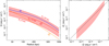 |
Fig. 2. Left panel: radial profiles of the volume cooling rate Q− (blue) and the volume heating rate Q+ from hydrodynamical (red; |


The above inference elicits two remarks. One is the projection effect, as the spherical velocity profile of v is obviously different from its projected profile to be observed. However, this effect is considered to be minor as in the deprojection analysis of the ICM temperature. The other is the expected radial decrease of Rint, due to the inward decrease of the fraction of gas-richer galaxies. This effect can be taken into account by replacing ngal in Eq. (13) with the number density of blue galaxies,  . According to Barkhouse et al. (2009), the ratio
  becomes halved at the center, but a 20% increase toward the center is observed in the ratio vB/v (Bilton & Pimbblet 2018), where vB is the velocity dispersion of blue galaxies. Thus, Q+/Q− would still be relatively flat within a factor of a few.
To verify the above estimates, we quantitatively computed Q+ and Q− based on actual observations. That is, Q− was calculated as a function of R, using the radial profiles of the ICM density, temperature, and the metallicity, all averaged over the 340 clusters with z = 0.0−0.5 from Gu et al. (2016). Similarly, in calculating Q+, its hydrodynamical contribution, denoted as  , was evaluated using the sample-average profiles of ngal and ρ also from Gu et al. (2016), and the mean v profile for a sample of ten cool-core clusters in Bilton & Pimbblet (2018, their Fig. 4, right panel). Although
  consists of the ram pressure (Eq. (6)) and the viscous friction (Eq. (7)) terms, the latter was neglected as argued in Sect. 3.3. The largest uncertainty in
  is the value of Rint, which should depend on the types of galaxies, and possibly on stages of the infalling process as well. In Fig. 2 (left), we therefore calculated
  for three typical cases, Rint = 5 kpc, 10 kpc, and 20 kpc. Thus, for a fixed value of Rint, the
  and Q− profiles indeed depend very similarly on R from the cluster center to ∼1 Mpc, and the
  ratio is close to unity if Rint is in between 10 and 20 kpc. We have assumed that all the dynamical energy losses from galaxies are in the end thermalized; if this is not the case, the
  profile needs to be scaled by the thermalization efficiency.
The g-mode interaction (Eq. (8)) is essential for a complete view of the heating. Although this process converts the dynamical energy of moving galaxies primarily into those of DM, the produced fluctuations (both in time and position) of the local gravitational potential would ultimately be spent in the ICM heating (via sloshing and similar effects). As the g-mode strength depends critically on the galaxy mass, we estimated it separately for two galaxy subsets: low-mass galaxies with mgal ≤ 1011 M⊙, and the remaining high-mass galaxies. For each subset, we calculated Eq. (8), again using the mass-sorted average ngal profiles from Gu et al. (2016) and the v profiles from Bilton & Pimbblet (2018). The ρtot information, also taken from Gu et al. (2016), is common to the two subsets. As shown in Fig. 2 (left), the heating rate  from the gravitational interaction, summed over the two subsets, has a more centrally peaked profile than
  because of several effects, for example, the more concentrated profile of ρtot than ρ, and a stronger central clustering of massive galaxies. In short, the g-mode interaction may contribute significantly to the heating at the core region, assuming efficient dissipation of DM fluctuations on the ICM, but much less relevant outside it.
In Fig. 2 (right), we directly compare, at each R, Q− against the total heating rate,  . Although the uncertainties from Rint are again large, we confirm an approximate balance between the two quantities. Thus, the galaxy-driven heating scenario has been shown to be matched very well with the R-dependent ICM cooling rate, if Rint takes a value of ∼10 kpc, which is suggested by the observed cosmological galaxy infall (Sect. 3.2.2; Gu et al. 2016).
The quantitative verification in Fig. 2 may still leave us with one basic question. The ICM thermal energy in the core region is far insufficient to sustain the X-ray emission against its short cooling time; indeed, this motivated the cooling-flow hypothesis. This leads us to the question of how the sustained heating would be available by the galaxies in the core region, of which the dynamical energy content must be at most comparable to the ICM thermal energy therein. The answer can be obtained if we notice that an appreciable faction of these galaxies must have larger orbits and happened to be near the center at present, rather than localized therein. As already considered in the orbital calculation by Gu et al. (2013a), such a galaxy repeatedly crosses the core with a typical interval of ∼0.1 tH, and lose, in every crossing, a small fraction (∼10%) of its dynamical energy. Thus, the heating energy can be supplied by member galaxies which are distributed over a much larger volume than the cluster core; the energy budget discussed so far in Sects. 3.2.2 and 3.3 should be understood in this context.
The essential difference between the dynamical energy of the galaxies and the ICM thermal energy is that the former can be transported by the ballistic motions of galaxies on a timescale of ∼0.1 tH, whereas the latter must be transported via electron conduction, which would take ∼tH for l ∼ 1 Mpc. In other words, galaxies are cooled globally because a considerable fraction of the overall galaxies participate in the core heating, whereas the ICM would be cooled (if no heating) very locally.
4. ICM turbulence
4.1. Galaxy motion and ICM turbulence
Here we investigate in a semi-quantitative way the behavior of ICM turbulence, which is expected to play an important role in the ICM heating from galaxy motion.
4.1.1. Overview
As shown in Sect. 1 and by Hitomi Collaboration (2018a), the ICM in the Perseus cluster core was revealed by Hitomi to be amazingly quiet. The observed spatial field of the ICM velocity dispersion is roughly composed of two components: a flat field of ∼100 km s−1 spreading on a ∼100 kpc scale and regions of enhancement to ∼200 km s−1 in the innermost 20 kpc and at an AGN-inflated bubble. Although the direct AGN feedback might be responsible for the latter, the origin of the former is still unclear. Therefore, other possibilities are being explored. For instance, ZuHone et al. (2018) propose that the turbulence originates from sloshing motion of the Perseus cool core, in response to gravitational perturbations by infalling subclusters. In this model, the gas motion is fully explained by the energy input from subcluster mergers. A similar scenario was proposed by Inoue (2014).
In this section, we employ our assumptions D1−D3 to explore a somewhat different idea that the ICM turbulence is mainly produced by the galaxy motion. Obviously, the effects of moving galaxies are less energetic than the mergers, but much more frequent and ubiquitous. We then try to answer the core question of the paper concerning whether this scenario is capable of explaining the essence of the Hitomi measurement.
The dynamical energy of moving galaxies is transferred to the ICM entropy through at least three channels. One is direct ICM heating via, for example, anomalous Joule dissipation of galaxy-induced electric currents. Another is a channel wherein the energy of the galaxies is first converted to kinetic energies of local ICM motions, which are then dissipated as ICM entropy. The other is an electromagnetic channel, such as amplification of magnetic fields and excitation of Alfvénic waves; these energies are transmitted to individual particles, through, for example, magnetic reconnection and wave damping. Below, we only consider only the second channel, which is thought to be dominant (Norman & Bryan 1999; Dennis & Chandran 2005).
The local ICM motions induced by galaxies that are moving with transonic velocities take the form of, for example, sound waves, vorticity around individual galaxies, and wakes trailing behind these galaxies (Vijayaraghavan & Ricker 2017), that is, ICM turbulence. The energy injection to the turbulence would take place on spatial scales of galaxies, for example, through a process known as resonant drag instability (Seligman et al. 2019) in which plasma perturbations are enhanced when the velocity of the galaxy matches the phase velocity of propagating perturbations (e.g., sound waves in this case). The turbulence then spreads through the ICM and splits down to smaller scales via the turbulence cascades. Although the scenario is thus simple, the details of turbulence in a compressible and magnetized plasma are rather complicated. Therefore, below we discuss only general aspects of the problem.
4.1.2. Characterization of the observed turbulence
We begin by comparing four characteristic velocities involved. The first example is the sound velocity s in the ICM, which takes a value as
 (14)
(14)
where γ = 5/3 is the adiabatic index and the temperature of T = 5 keV applies to the Perseus cluster (the hot component). For simplicity, the plasma is approximated as hydrogenic. The second example is the velocity dispersion of the galaxies, denoted as v as before, which is comparable to s as widely recognized.
The third is the Alfvén velocity, given as
 (15)
(15)
where the magnetic-field intensity B = 5 μG and the ICM density ne = 10−2 cm−3 used for normalization are both appropriate in the Perseus core region. The plasma beta, that is, the thermal gas pressure relative to the magnetic pressure, becomes
 (16)
(16)
The last item is just the ICM turbulence velocity dispersion, σ ∼ 160 km s−1 as measured with Hitomi. Therefore, we find
 (17)
(17)
In short, the galaxy motion is transonic but super-Alfvénic, whereas the ICM turbulence is subsonic but trans-Alfvénic. It is noteworthy that the measured σ is close to the calculated vA.
Because v ∼ s holds, the moving galaxies are not expected to create strong shocks in the ICM. Because v ≫ vA, neither do they produce so-called slow shocks (discontinuities in the slow-mode longitudinal waves) to be realized with sub-Alfvénic plasma flows. In the regime of Eq. (17), instead, each moving galaxy bends MFLs and create kinks in them, where thin sheets of electric currents should be formed. These current sheets are expected to provide promising sites, where the turbulence and electromagnetic energies are efficiently dissipated, for example, via magnetic reconnection and Joule heating.
Under the condition of Eq. (17), the turbulence propagates through the ICM with two modes: the longitudinal sound waves and the transverse shear (or torsional) Alfvén waves. Since s ≫ vA, the magnetosonic velocity  is essentially the same as s. Although MFLs are perturbed by these fluctuations, we do not expect strong entanglement of these fluctuations because the turbulence is trans-Alfvénic. Therefore, the ordered MFL structure assumed in S1 should remain valid.
4.1.3. Expected turbulence velocity dispersion
As described in Sect. 4.1.1, we assume that the energy ΔEgal of Eq. (4) mostly flows through the channel of ICM turbulence before dissipated into entropy, and that this provides the dominant heating source for the ICM. Then, the energy temporarily stored at present in the form of ICM turbulence must be a certain fraction of ΔEgal. As a result, the ICM turbulence velocity dispersion σ satisfies  , where MICM is the total ICM mass. We hence obtain from Eq. (4),
 (18)
(18)
In short, the turbulence due to the galaxy motion must be subsonic in a rich cluster, in agreement with the Hitomi results.
The above argument can be formulated in a more generalized context. If we suppose that the energy of galaxies, Eq. (1), is transferred, on a timescale of τ1 (Eqs. (2) and (9)), to the ICM turbulence energy, which in turn is dissipated into entropy (Zhuravleva et al. 2014) on another timescale τ2. If the overall energy flow is in an approximate steady state, we should expect
 (19)
(19)
This yields an estimate, averaged over each cluster, as
 (20)
(20)
where we employed v ∼ 1000 km s−1 after Eq. (14), and Mgal/MICM ∼ 0.3, which is appropriate for a cluster-averaged estimate. This is consistent with Eq. (18), if τ2/τ1 ≲ 0.3.
For a further estimate focusing on the core region, we assume that the turbulence is dissipated on its crossing timescale, namely, τ2 ∼ ltur/σ, where ltur is the largest driving scale (injection scale) of the turbulence, which may be taken to be the length scale of galaxies, lgal ∼ 20 kpc (Zhuravleva et al. 2014, 2018). The general consistency between dissipation and crossing timescales for compressible and subsonic MHD turbulence has been validated by numerical simulations as reported in, for example, Haugen et al. (2004). Substituting this into Eq. (20), and solving it for σ, we obtain
 (21)
(21)
where we used the estimate τ1 ∼ 0.1 tH, which applies to the cluster core as noticed just after Eq. (9). The first factor, (Mgal/MICM)c, is the galaxy-to-ICM mass ratio in the core region, which may be taken as ∼1. Thus, the predicted turbulence velocity is fully consistent with the Hitomi measurement, considering various uncertainties involved in Eq. (21).
From these values of σ, we obtain
 (22)
(22)
in the core region. Therefore, the ICM turbulence therein is inferred to dissipate on a timescale comparable to the cooling time at the very center, ∼6 × 10⁻³ tH. As a corollary to Eq. (22), we find
 (23)
(23)
which means that about 10% of the dynamical energies of galaxies in the core region is stored temporarily as the ICM turbulence energy. Although this value is rather small, as evident from the Hitomi results, this turbulence energy can sustain the ICM entropy against the radiative cooling because it is continuously replenished by a large number of galaxies, some of which have larger orbits and happened to be in the core region.
4.1.4. Spatial uniformity of turbulence
At this stage, the remaining task is to examine whether the proposed scenario can also explain the observed uniformity of σ, on spatial scales from ∼20 kpc to ∼100 kpc. We may first consider the uniformity on rather small spatial scales as < 20 kpc. The ICM turbulence created by a single galaxy would only occupy a limited cluster volume localized around its trajectory. However, in a massive cluster with numerous galaxies crossing the core region, their loci, each with a typical width of 20 kpc (Roediger et al. 2015), fill up nearly the entire core volume in ∼108 yr, which is the timescale on which the turbulence is dissipated according to Eq. (22). Therefore, when averaged for ≫108 yr, the ICM turbulence would be rather uniform within the cluster core region (Subramanian et al. 2006).
We next consider how σ would depend on R on relatively large scales as > 50 kpc. For this purpose, webreak up the argument in Sect. 3.3.3, and consider the behavior of σ as a quantity intervening between the heating and cooling. Supposing that Q+ and Q− are approximately balanced as in Fig. 2, the steady-state condition of the turbulence is then described, from Eq. (12), as
 (24)
(24)
which yields  as ρ cancels out. Further approximating both Rint and v as spatially constant, we obtain
 (25)
(25)
Therefore, the problem reduces to the behavior of τ2.
If the fluid were incompressible, τ2 would depend neither on the mean fluid density nor the turbulence strength. However, its behavior becomes different in the ICM, which is clearly compressible. According to a theoretical study by Yoshizawa et al. (1997), the turbulence dissipation in a compressible and low-Mach number fluid is a nonlinear phenomenon, so that τ2 gets shorter as σ increases. For simplicity, we may describe this effect as τ2 ∝ σ−k, using an empirical index k > 0. Combining this with Eq. (25), we obtain
 (26)
(26)
If assuming k ∼ 1 (following Eq. (21)), σ would vary by only a factor of ∼2 over a spatial scale of several hundred kiloparsec, across which ngal changes by an order of magnitude as in Fig. 1 (left).
In addition to the MHD processes as above, the infalling massive galaxies can also create the ICM turbulence by exciting gravity (g-mode) waves (Balbus & Soker 1990; Ruszkowski & Oh 2011) as in Eq. (8). In this case, the galaxies pulls, through dynamical friction, the local DM and ICM away from their original positions, and their restoration by gravity and sound waves creates a low-frequency oscillation in the ICM. As the galaxies gradually fall toward the cluster center, the resulting g-mode waves also propagate inward and fill the cluster core volume. Through the same argument as above but using Eq. (8) instead of Eq. (6), we obtain, in place of Eq. (25),
 (27)
(27)
where mgal and v were approximated as constant. Therefore, corresponding to Eq. (26), we obtain
![Mathematical equation: $$ \begin{aligned} \sigma \propto \left[ n_{\rm gal} \, (\rho _{\rm tot}/\rho ) \right]^{1/(k+2)}. \end{aligned} $$](/articles/aa/full_html/2020/06/aa36437-19/aa36437-19-eq48.gif) (28)
(28)
As the ratio ρtot/ρ depends only mildly on R, the expected behavior of σ is again similar to the case of Eq. (26). In summary, our scenario can explain, not only the value of σ, but to some extent the observed uniformity of σ as well.
4.2. Numerical simulations
Among many numerical simulations of the astrophysics of clusters of galaxies, the effects of magnetic fields on the galaxy versus ICM interaction have only been addressed by a few studies, including Asai et al. (2004, 2006, 2007), Dursi & Pfrommer (2008), and Suzuki et al. (2013). In the MHD framework that takes into account radiative cooling and anisotropic heat conduction, these authors studied interactions between a uniformly inflowing ICM, and a denser plasma gravitationally confined in a simulated galaxy. This numerical setup is similar to the condition considered in Sect. 3.3, although their model galaxy is a kind of intermediate between a cD galaxy and a moving member in our scenario. These authors have found several essential features, including the excitation of MHD turbulence on spatial scales of the galaxy, formation of loop-shaped cooler regions around it, and a suppression of radiative cooling. These results are in support of our scenario.
The g-mode interaction between the member galaxies and the ICM was studied with a three-dimensional simulation by Ruszkowski & Oh (2011). Although they treated the ICM in an MHD scheme, they ignored (magneto-)hydrodynamical interactions between the ICM and galaxies. The gas motion in the simulated clusters was found to have a velocity of 100−200 km s−1, which agrees well in with the Hitomi measurements. The cluster-average gas motion approximately scaled as R−1/2, which is qualitatively similar to Eq. (28) assuming ngal ∼ R−(k + 2)/2.
Based on the above simulation, Ruszkowski & Oh (2011) calculated the heating luminosity of the cool core, in a similar way to those in Sect. 4.1.3, as
 (29)
(29)
where Vcc and Rcc are the volume and radius of the cool core, respectively, and ltur ∼ 150 kpc is the typical length scale of turbulence they found in their simulations. This ltur is considerably longer than the dissipation length, lgal ∼ 20 kpc, which we have assumed so far. Consequently, Lcc fell below the cooling luminosity of the CCC of rich clusters (Table 1). If, however, the MHD interactions between the galaxies and ICM are properly taken into account, ltur could become much shorter, fopr example, down to ltur ∼ lgal as we assumed, and hence Lcc could increase.
In spite of the insufficient heating by Lcc, the runaway cooling was interestingly suppressed in the simulation of Ruszkowski & Oh (2011). The authors discuss a possibility of heat inflow from outer to inner regions via heat conduction and/or turbulent diffusion (Ruszkowski & Oh 2011). Therefore, it is suggested that the ICM cooling in the core region is at least partially offset by such inward heat transport from outer regions.
More recently, the combined MHD and g-model interactions between the ICM and moving galaxies were studied numerically, with an adaptive-mesh MHD approach, by Vijayaraghavan & Ricker (2017). Their results (particularly movies) clearly reveal that each galaxy strongly interacts with the ICM, deposits cooler ISM onto the intracluster volume, and produces ICM turbulence on spatial scales of galaxies or less. Most of the clusters they simulated are mildly turbulent (σ = 50−300 km s−1) within the central ∼500 kpc. In addition, the gas motion is volume filling and reasonably isotropic on large scales. Thus, the work by Vijayaraghavan & Ricker (2017) can successfully explain the Hitomi measurements in terms of the galaxy-ICM interaction and provides a convincing support of our viewpoint. This work also suggests that the galaxy-ICM interaction systematically amplifies the cluster magnetic fields and drives magnetic evolution on cosmological timescales.
4.3. Other observations of ICM turbulence
Except the Hitomi results, successful observations of the ICM turbulence are so far still rare because of the obvious instrumental limitations. The reports are limited to a few observations using line broadening (Sanders et al. 2010; Pinto et al. 2015), resonant scattering (Ogorzalek et al. 2017), and surface brightness fluctuations (Zhuravleva et al. 2014) in central regions of brightest clusters of galaxies. These different approaches have well converged to a subsonic gas motion with σ = 100−300 km s−1. With the current data, however, it is not possible to isolate gas motions driven by the galaxy motion from those due to other excitation mechanisms such as buoyant motions from the feedback of the central AGN. A full understanding of the galaxy-ICM interaction needs to wait for dedicated spatially resolved observations with future high-resolution X-ray spectrometers.
Despite the paucity of direct evidence, there are already a few hints showing turbulence driven by galaxies. Optical and radio spectroscopic observations detected significant Doppler broadening in emission lines from the cool gas tails produced by ram pressure stripping, and the tail turbulence was measured in a few objects (Vollmer et al. 2006; McDonald et al. 2012). For instance, analyzing H I clouds that are ram pressure-removed from galaxies in the Virgo cluster, Abramson et al. (2011) derived the velocity dispersions of the clouds as a few tens of km s−1 to ∼150 km s−1 (Kenney et al. 2004), which is in broad agreement with the Hitomi measurement in Perseus. However, these should be treated as a consistency check, rather than direct evidence for our scenario, as the physical link between the tail turbulence and the ICM turbulence is still unclear.
Recently, Eckert et al. (2017) estimated the ICM turbulence in a sample of 51 clusters, indirectly through ICM density fluctuations, and found that the power of their radio halo depends depends on the turbulence as Pradio ∝ σ3.3. This scaling suggests a possible relation between the turbulent motions in the ICM and the population of accelerated particles. Then, by extrapolating the scaling to low-Pradio regimes, we can estimate σ on subcluster scales, assuming that the underlying physics should not be strongly scale dependent. Based on an Effelsberg 1.4 GHz observation, Vollmer et al. (2004) detected an extended radio halo of Pradio ∼ 1 × 10²² W Hz−1 centered on the giant elliptical M 86 in the Virgo cluster, and attributed the results to ongoing interactions between M 86 and the Virgo ICM. Then, the above scaling predicts the radio halo to have σ ∼ 100 km s−1. A similar extended radio halo is found centered on NGC 4839, which is a group of galaxies falling into the Coma cluster and emitting a 1.4 GHz radio power of 8 × 10²² W Hz−1 (Deiss et al. 1997). The scaling relation predicts σ ∼ 180 km s−1; these estimates are close to the Hitomi measurement.
To summarize, our scenario, that the mild ICM turbulence results from the galaxy-ICM interactions, has been supported from several aspects, including the ability to explain the value of σ (Sect. 4.1), a few numerical simulations (Sect. 4.2), and some indirect observations (Sect. 4.3).
5. Discussion
Previous studies of clusters of galaxies, either observational, theoretical, or numerical, treated the galaxies and the ICM almost independently, and interplay between them was considered only in rather limited aspects such as local stripping of galactic diffuse media. The present study, in contrast, has directly considered interactions between the high-density and low-entropy galaxies, and the low-density and high-entropy ICM, that is, the two major baryonic components of clusters. Thus, adopting the two sets of simple assumptions (Sects. 2.1 and 2.2), and considering the (magneto-) hydrodynamic and g-mode effects (Sect. 3.3), we developed the view that a large amount of energy flows from galaxies to the ICM, and that this phenomenon ubiquitously affects dynamics, energetics, and evolution of clusters. As summarized in Table 2, accumulating pieces of evidence lend supports to our overall scenario. Among these, of particular importance are the evidences of the cosmological galaxy infall (Sect. 3.2.2) and the consistency with the Hitomi results (Sect. 4). Our picture, however, has still two missing or inadequate pieces: first, how moving galaxies receive significant drag force from their host cluster, and second what maintains the thermal stability between the hot ICM and the cool core. Below, we address these two questions, where the first is a direct continuation from Sect. 3.3.2.
Evidence for the proposed scenario.
5.1. Force transmission via gravity
Although we thus far argued that moving galaxies experience a variety of ICM versus ISM interactions, a vital question still remains concerning how the inflowing ICM exerts drag force on the stellar and DM components that dominate the mass of each galaxy. For this purpose, we need to consider the role of gravity.
The most common form of gravitational interaction is the dynamical friction between each galaxy and the host cluster (Eq. (8)). If it is fully responsible for the possible GLIMR or GNIMR evolution (Sect. 3.2.2) reported in Gu et al. (2013a, 2016), we would naturally expect a mass-dependent radial segregation of member galaxies (Nath 2008). In addition, galaxies in high-ρtot environments would fall faster than those in low-ρtot systems. However, Gu et al. (2013a); Gu et al. (2016) found that the GNIMR (or GLIMR) profiles are not much different between brighter and fainter galaxy subsamples, or between lower-mass and higher-mass cluster subsamples. Strictly speaking, lower-mass galaxies are observed to fall to the cluster center somewhat less rapidly than the average galaxies (Gu et al. 2013a, 2016), but the difference is limited. It is therefore difficult to attribute the observed galaxy infall solely to the dynamical friction. This is consistent with the results presented in Fig. 2.
In this section, we introduce a new recipe for the ICM versus galaxy interaction, combining the hydrodynamical and gravitational effects. As shown by the numerical work of Roediger et al. (2015), the ram pressure by the inflowing ICM first strips a galaxy of its ISM, outside a radius where the ram pressure balances the gravitational restoration force (Gunn & Gott 1972). Then, within that radius and toward downstream of the galaxy, a long-lasting tail is formed by the ISM that survived the stripping. According to current observations (Sect. 3.1) and numerical simulations (Roediger et al. 2015), this displaced ISM tail (including new stellar populations born therein) is massive enough to gravitationally pull the whole stellar and DM components of the galaxy toward downstream, until the tail is fully stripped. In this way, the ICM can indirectly exert drag force to the nongaseous components of each moving galaxy.
Employing a simple analytic approach, we quantitatively examine whether the above idea works or not. The ISM tail may be approximated by a sphere of radius Rism with a uniform mass density ρism, which is displaced just by the same Rism from the potential center of the galaxy that has a mass of mg. Then, the gravitational restoration force working on the sphere is  . Equating this with the ram pressure
  working on the ISM sphere, where ρ is the ICM density as before, the critical radius for stripping is obtained as
 (30)
(30)
This is close to the stripping radius derived by McCarthy et al. (2008), based on more realistic distributions of ρtot and ρism.
In the above modeling, the ISM inside Rism is displaced downward, but is still bound to the galaxy and keeps receiving the ram pressure and transmitting it via gravity force to all the components of the galaxy. Therefore, this Rism can be identified with the interaction radius Rint in Eqs. (6) and (7). Numerically, we find
 (31)
(31)
where nism is the ISM number density corresponding to ρism in units of cm−3. This indeed justifies our assumption of Rint ∼ 10 kpc, employed when calculating the heating versus cooling balance in Fig. 2. Furthermore, the assumed ISM mass within Rism is  . This is only ∼0.1% of the assumed galaxy mass and would apply even to elliptical galaxies. Elliptical galaxies residing in a cluster core region may have a lower value of nism, but then the dynamical friction supersedes. Overall, the ram pressure effect on a member galaxy closely resembles the drag force exerted on a smooth solid body placed in a flowing fluid.
Equation (30) implies that Rism scales with mgal, as a simple consequence of larger binding energies in more massive galaxies. Then, like the dynamical friction case, this might appear to predict a strong mgal dependence of the cosmological galaxy infall and contradict to the results of Gu et al. (2013a); Gu et al. (2016). However, the estimated Rism is already close to the size of galaxies, so it would not increase very much even for more massive galaxies. Furthermore, galaxies with smaller mgal, mostly spirals, would have higher nism, which would partially compensate for the lower mgal. Therefore, we expect relatively weak mgal dependence of the proposed ICM versus galaxy interaction mechanism, which agrees with the actual observations.
While the above estimate only assumes the hydrodynamical effect, in reality we need to take into account the magnetic fields both in the ICM and galactic ISM. For example, MHD simulations of the ram pressure interactions by Ruszkowski et al. (2014) and Shin & Ruszkowski (2014) show a compression of upstream galactic magnetic fields that are exposed to the incoming ICM flow. The consequent smaller gyroradius makes it even harder for the ICM particles to flow through interstellar space. Furthermore, MFLs in the ICM could be draped around each moving galaxy (Vijayaraghavan & Ricker 2017) and effectively increase Rint.
5.2. Temperature and thermal stability of the CCC
Although we have thus far assumed the core-region ICM to be homogeneous, in reality we need to consider the 2P structure found therein (Sect. 2.1), consisting of the hot phase and the cool phase (i.e., CCC). As postulated in our static assumptions, the two phases are likely to be thermally insulated by MFLs, and intermixed on spatial scales of ∼10 kpc in an approximate pressure equilibrium. These 2P regions of typical clusters still dominate by the hot phase and the CCC occupies only a small (<20%) fraction of the volume (Ikebe et al. 1999; Takahashi et al. 2009; Gu et al. 2012) except the central a few tens kiloparsec where the cD galaxy dominates. Therefore, the heating luminosity Q+ in Fig. 2 must be deposited mainly on the hot phase and the generated heat is carried along MFLs by the electron conduction and turbulence propagation on timescales of 106 years (Gu et al. 2012) and Eq. (22), respectively. As a result, the hot phase becomes isothermal throughout the core region, as confirmed by observations (Ikebe et al. 1999; Takahashi et al. 2009; Gu et al. 2012).
Although the electron conduction would not work between the two phases, the ICM turbulence excited in the hot phase by galaxies perturbs, from outside, the magnetic flux tubes that confine the CCC (see Eqs. (16) and (17)). The turbulence can hence propagate from the hot phase into the cool phase across the MFLs to be dissipated efficiently on the CCC, which has a higher density. In addition, sometimes galaxies would pass through the cool phase, directly excite the turbulence therein, and disturb the magnetospheric structure. These processes are considered to provide the CCC with the necessary heating luminosity.
Two immediate questions are how Q+ is divided into the two phases so as to match their respective X-ray luminosities and how the 2P configuration is kept thermally stable for much longer than the nominal cooling time. These related questions stem from the fact that the volume cooling rate of a plasma is proportional to  as in Eq. (11), whereas the rate of any heating mechanism would be proportional to ne (e.g., Eq. (12)). Then, if the energy deposit on the cool phase is lower than its X-ray output luminosity, the cool phase would lose pressure, be compressed to become denser, and would cool more rapidly. The cool phase would collapse in ∼0.1 tH or shorter. This is virtually identical to the initial cooling-flow problem.
The assumption S3 made in Sect. 2.1 helps us to avoid the above difficulty because the CCC confined within thin magnetic flux tubes can be made thermally stable (Paper I; Takahashi et al. 2009; Gu et al. 2013b), by so-called RTV mechanism as quoted in our assumption D4. Originally proposed for solar coronae by Rosner et al. (1978), it was improved by Aschwanden & Schrijver (2002), and confirmed in actual observations with the Solar Observatory Yohkoh (Kano & Tsuneta 1996). This mechanism assumes that a plasma is (1) confined by some external pressure, (2) within a thin magnetic loop, (3) in a hydrostatic equilibrium, and (4) is heated from outside. The conditions (1), (2), and (4) are satisfied by our CCC view. The condition (3) is also likely to hold because the filamentary structures in the Perseus and Centaurus clusters have constant internal pressures (Fabian et al. 2005; Sanders et al. 2016), so the momentum flows through the filaments are considered rather small.
The RTV mechanism further postulates that the plasma within the tube is cooled by the X-ray radiation, and by MFL-aligned classical heat conduction toward the two footpoints. Then, if the cooling overwhelms the heating, the tube becomes thinner because of the reduced internal pressure, so the conductive flux along the tube decreases. In addition, a part of the plasma flows into the footprints to reduce the radiative output. Thus, the CCC achieves a new equilibrium with a reduced cooling luminosity, while the plasma temperature remains rather unchanged. Conversely, when the heating overcomes the cooling, the magnetic tubes expand, and additional plasma is supplied by the cD galaxy into the tubes. These lead to a higher radiative and conductive cooling, which balances the excess heating. The CCC thus responds to variations in the heating luminosity, by adjusting its X-ray radiative output, rather than changing the temperature. As a result, the 2T configuration keeps the required thermal stability.
In addition to the above evaluation, we have more quantitative support indicating that the RTV mechanism is working in cD clusters. The RTV theory predicts a scaling law: the temperature inside the magnetic loops is determined by the loop half length H and the confining pressure p0 (the hot phase pressure in the present case), without depending on the heating or cooling luminosity (Rosner et al. 1978; Aschwanden & Schrijver 2002). Then, according to Takahashi et al. (2009) and Gu et al. (2012), the maximum temperature of the plasma confined within a cool-core-sized magnetic loop is predicted as
![Mathematical equation: $$ \begin{aligned} T_{\rm c}^\mathrm{max} = (2.0-2.5) \left[ \left( \frac{p_0}{10^{-10}} \right) \left( \frac{H}{30\,\mathrm{kpc}} \right) \right]^{1/3}\,\mathrm{keV}, \end{aligned} $$](/articles/aa/full_html/2020/06/aa36437-19/aa36437-19-eq56.gif) (32)
(32)
where p0 is in units of dyn cm−2. Considering that this  refers to the loop-top temperature, and the volume-averaged loop interior must be somewhat cooler (Gu et al. 2012), the average CCC temperature is expected to be 1−2 keV, in very good agreement with what is observed from typical cool core clusters. Further considering the hot phase properties, Takahashi et al. (2009) derived a theoretical scaling relation as
  , which can approximately reproduce the empirical scaling relation of Tc = (0.4−0.6) Th (Allen et al. 2001; Kaastra et al. 2004). These results strongly support to our assumption D4 because no other convincing explanation has ever been given either to the value of Tc or its dependence on Th.
5.3. Outlook: XRISM and Athena
The X-Ray Imaging and Spectroscopy Mission (XRISM; to be launched in 2022), planned as a successor to Hitomi, carries an X-ray micro-calorimeter that is nearly identical to that on Hitomi. Beyond that, we can look forward to Athena (Nandra et al. 2013, early 2030s) with even higher spectral resolution and better sensitivity. These future X-ray missions extend the innovative Hitomi results on the Perseus cluster to many other systems, and provide breakthroughs in our understanding of the thermal evolution of the ICM. As noted in the XRISM mission concept paper (Tashiro et al. 2018), the scenario of ICM heating from galaxy motion becomes one of the feasible alternatives (but not necessarily mutually exclusive) to the AGN heating model, to be tested using XRISM. We describe these future prospects in two relevant aspects.
5.3.1. Galaxy-ICM coupling
Our scenario predicts that a fast-moving bright galaxy partially drags the local ICM around it. This prediction can be tested, in principle, by comparing the local X-ray redshifts around bright member galaxies with their optical line-of-sight peculiar motions (e.g., Wittmann et al. 2019).
One of the best efforts to detect the above effect, using the X-ray CCD, was made by Tamura et al. (2014) for the Perseus cluster. By analyzing the well-calibrated Suzaku Fe-K data, the authors determined the radial velocities of the ICM in a spatial mesh of ∼50−100 kpc over a central 600 kpc region, with an instrumental systematic uncertainty of ∼300 km s−1, and compared the ICM motion with the optically measure galaxy velocities. Despite the limited energy resolution of CCD, their work discovered a mild positive correlation between the two components in their line-of-sight motions. Similarly, a tentative correlation has been reported by Yu et al. (2016) for A 85. The Hitomi spectrum has the sufficient energy resolution to determine the ICM bulk motion within a few tens km s−1 (Hitomi Collaboration 2018a), but the observed region was too small to cover a sufficient number of non-cD galaxies in Perseus.
To finally verify the possible galaxy-ICM coupling, it is essential to map the ICM motion accurately over a large area. We hence simulated a mosaic XRISM observation of the Perseus cluster based on the Suzaku measurement by Tamura et al. (2014). The XRISM spectra were simulated for ∼80 pointings, using the temperature and density profiles in Zhuravleva et al. (2014) and the abundance profile in Werner et al. (2013). A systematic uncertainty by 1 eV, arising from gain calibration limitations, was taken into account. Even with a short 30 ks exposure for each pointing, we confirmed that the XRISM spectrum can determine the ICM Doppler redshift within ∼50 km s−1, up to a large radius of 600 kpc from the cD galaxy. By comparing the X-ray data from ∼80 pointings with the existing optical survey data (e.g., Huchra et al. 1995, 2012), we expect we can derive a meaningful answer to the prediction.
5.3.2. Ram pressure
As described in Sect. 4, we expect that the ram pressure and the related MHD effects are at least partially responsible for the observed turbulence in the cluster central region. This scenario is supported by some of the latest simulations (e.g., Fig. 5 of Roediger et al. 2015; Vijayaraghavan & Ricker 2017), which show that both the stripped ISM and downstream ICM are perturbed by the ram pressure effect to become more turbulent.
The micro-calorimeters on board the upcoming XRISM and Athena missions provide the first direct test to the above predictions. In this work, we show a simulation of the expected results for a candidate target, M 86, which is a nearby elliptical galaxy falling into the Virgo cluster with a line-of-sight impact velocity of ∼1500 km s−1. This galaxy hosts the brightest ram pressure tail in X-ray and Hα, with a length of ∼150 kpc in projection. High-resolution X-ray spectra of the upstream, tail, and the downstream regions (see Fig. 3 for their rough locations) enable us to search for possible turbulence caused by M 86, and to constrain its energy injection to the ICM. The simulation employs the temperature, abundances, and emission measures of the M 86 ISM, as well as of the surrounding Virgo ICM, as measured with Suzaku (Hishi et al. 2017). Assuming that the turbulence is 165 km s−1 (Hitomi Collaboration 2016) at the upstream, and is boosted by Δσ = 400 km s−1 at the tail and downstream, the enhancement would be detected with XRISM if we invested rather long exposures, ∼400 ks at the upstream and downstream, and 100 ks at the tail. With Athena, a much reasonable exposure of ∼20−30 ks each region would be sufficient to detect the turbulence enhancement at the 3σ confidence level. For lower contrast, for example, for Δσ = 200 km s−1, a longer exposure will be needed; 1 Ms with XRISM and 60 ks with Athena.
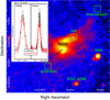 |
Fig. 3. Image by ROSAT of M 86 region. The approximate direction of M 86 motion is denoted by a black arrow. The green boxes show the field of views of the simulated XRISM/Athena spectra for the upstream, tail, and downstream regions. Inset: simulated XRISM (left, 400 ks) and Athena (right, 30 ks) spectra of a narrow band around the blended Ne X and Fe XXIII lines at 1.017 keV. The turbulence in the downstream region (red) is assumed to be 565 km s−1, higher than that in the upstream region (black) by Δσ = 400 km s−1. |
6. Summary
Based on a number of data-oriented X-ray studies, and by adopting simple assumptions on the static and dynamical aspects, we develop a physical model that involves the member galaxies to interact with the cluster environment (particularly the ICM) through ram pressure, g-mode, and other MHD effects. As a result, a large amount of energy is expected to flow from the moving galaxies into the ICM, first in a form of turbulence, which then dissipates into heat that may significantly offset the long-term radiative cooling of the ICM. The evidence of cosmological infall of member galaxies, which is a natural consequence of the above view, has been found in previous works. Our scenario is also well in line with the recent Hitomi result because the galaxy-ICM interaction predicts a mild subsonic turbulence with a good spatial uniformity, just as observed with Hitomi. We speculate that the galaxy-ICM interaction might be universally present across the cluster field, creating a significant and persistent energy flow in the present Universe.
Acknowledgments
L.G. is supported by the RIKEN Special Postdoctoral Researcher Program. SRON is supported financially by NWO, the Netherlands Organization for Scientific Research. H.X. acknowledges the supports of the National Natural Science Foundation of China (grant nos. 11621303, 11835009, 11973033) and the Ministry of Science and Technology of China (grant nos. 2018YFA0404601).
References
- Abadi, M. G., Moore, B., & Bower, R. G. 1999, MNRAS, 308, 947 [NASA ADS] [CrossRef] [Google Scholar]
- Abramson, A., Kenney, J. D. P., Crowl, H. H., et al. 2011, AJ, 141, 164 [NASA ADS] [CrossRef] [Google Scholar]
- Allen, S. W., Schmidt, R. W., & Fabian, A. C. 2001, MNRAS, 328, L37 [NASA ADS] [CrossRef] [Google Scholar]
- Armitage, T. J., Barnes, D. J., Kay, S. T., et al. 2018, MNRAS, 474, 3746 [CrossRef] [Google Scholar]
- Asai, N., Fukuda, N., & Matsumoto, R. 2004, J. Korean Astron. Soc., 37, 575 [CrossRef] [Google Scholar]
- Asai, N., Fukuda, N., & Matsumoto, R. 2006, Astron. Nachr., 327, 605 [CrossRef] [Google Scholar]
- Asai, N., Fukuda, N., & Matsumoto, R. 2007, ApJ, 663, 816 [NASA ADS] [CrossRef] [Google Scholar]
- Aschwanden, M. J., & Schrijver, C. J. 2002, ApJS, 142, 269 [NASA ADS] [CrossRef] [Google Scholar]
- Bahcall, N. A. 1999, in Formation of Structure in the Universe, eds. A. Dekel, & J. P. Ostriker, 135 [Google Scholar]
- Balbus, S. A., & Soker, N. 1990, ApJ, 357, 353 [NASA ADS] [CrossRef] [Google Scholar]
- Balogh, M. L., Schade, D., Morris, S. L., et al. 1998, ApJ, 504, L75 [NASA ADS] [CrossRef] [Google Scholar]
- Balogh, M. L., Baldry, I. K., Nichol, R., et al. 2004, ApJ, 615, L101 [NASA ADS] [CrossRef] [Google Scholar]
- Bambic, C. J., Morsony, B. J., & Reynolds, C. S. 2018, ApJ, 857, 84 [CrossRef] [Google Scholar]
- Barkhouse, W. A., Yee, H. K. C., & López-Cruz, O. 2009, ApJ, 703, 2024 [NASA ADS] [CrossRef] [Google Scholar]
- Bilton, L. E., & Pimbblet, K. A. 2018, MNRAS, 481, 1507 [CrossRef] [Google Scholar]
- Böhringer, H., Chon, G., & Kronberg, P. P. 2016, A&A, 596, A22 [NASA ADS] [CrossRef] [EDP Sciences] [Google Scholar]
- Bösch, B., Böhm, A., Wolf, C., et al. 2013, A&A, 549, A142 [NASA ADS] [CrossRef] [EDP Sciences] [Google Scholar]
- Bourne, M. A., & Sijacki, D. 2017, MNRAS, 472, 4707 [NASA ADS] [CrossRef] [Google Scholar]
- Brunetti, G., & Lazarian, A. 2007, MNRAS, 378, 245 [NASA ADS] [CrossRef] [Google Scholar]
- Budzynski, J. M., Koposov, S. E., McCarthy, I. G., McGee, S. L., & Belokurov, V. 2012, MNRAS, 423, 104 [NASA ADS] [CrossRef] [Google Scholar]
- Butcher, H., & Oemler, A., Jr. 1984, ApJ, 285, 426 [NASA ADS] [CrossRef] [Google Scholar]
- Cappellari, M., Bacon, R., Bureau, M., et al. 2006, MNRAS, 366, 1126 [NASA ADS] [CrossRef] [Google Scholar]
- Chandran, B. D. G., & Rasera, Y. 2007, ApJ, 671, 1413 [NASA ADS] [CrossRef] [Google Scholar]
- Churazov, E., Brüggen, M., Kaiser, C. R., Böhringer, H., & Forman, W. 2001, ApJ, 554, 261 [NASA ADS] [CrossRef] [Google Scholar]
- Clarke, T. E. 2004, J. Korean Astron. Soc., 37, 337 [NASA ADS] [CrossRef] [Google Scholar]
- Conselice, C. J., Gallagher, J. S., III, & Wyse, R. F. G. 2001, AJ, 122, 2281 [NASA ADS] [CrossRef] [Google Scholar]
- Couch, W. J., Barger, A. J., Smail, I., Ellis, R. S., & Sharples, R. M. 1998, ApJ, 497, 188 [NASA ADS] [CrossRef] [Google Scholar]
- Crawford, C. S., Sanders, J. S., & Fabian, A. C. 2005, MNRAS, 361, 17 [NASA ADS] [CrossRef] [Google Scholar]
- de Plaa, J., Kaastra, J. S., Werner, N., et al. 2017, A&A, 607, A98 [NASA ADS] [CrossRef] [EDP Sciences] [Google Scholar]
- Deiss, B. M., Reich, W., Lesch, H., & Wielebinski, R. 1997, A&A, 321, 55 [NASA ADS] [Google Scholar]
- Dennis, T. J., & Chandran, B. D. G. 2005, ApJ, 622, 205 [NASA ADS] [CrossRef] [Google Scholar]
- Dressler, A. 1980, ApJ, 236, 351 [NASA ADS] [CrossRef] [Google Scholar]
- Dursi, L. J., & Pfrommer, C. 2008, ApJ, 677, 993 [NASA ADS] [CrossRef] [Google Scholar]
- Eckert, D., Gaspari, M., Vazza, F., et al. 2017, ApJ, 843, L29 [NASA ADS] [CrossRef] [Google Scholar]
- Eilek, J. A., & Owen, F. N. 2002, ApJ, 567, 202 [NASA ADS] [CrossRef] [Google Scholar]
- Enßlin, T. A., & Vogt, C. 2006, A&A, 453, 447 [NASA ADS] [CrossRef] [EDP Sciences] [Google Scholar]
- Fabian, A. C. 1994, ARA&A, 32, 277 [NASA ADS] [CrossRef] [Google Scholar]
- Fabian, A. C. 2012, ARA&A, 50, 455 [NASA ADS] [CrossRef] [Google Scholar]
- Fabian, A. C., Sanders, J. S., Ettori, S., et al. 2000, MNRAS, 318, L65 [NASA ADS] [CrossRef] [Google Scholar]
- Fabian, A. C., Sanders, J. S., Ettori, S., et al. 2001, MNRAS, 321, L33 [NASA ADS] [CrossRef] [Google Scholar]
- Fabian, A. C., Sanders, J. S., Allen, S. W., et al. 2003, MNRAS, 344, L43 [NASA ADS] [CrossRef] [Google Scholar]
- Fabian, A. C., Sanders, J. S., Taylor, G. B., & Allen, S. W. 2005, MNRAS, 360, L20 [NASA ADS] [CrossRef] [Google Scholar]
- Fabian, A. C., Sanders, J. S., Taylor, G. B., et al. 2006, MNRAS, 366, 417 [Google Scholar]
- Fabian, A. C., Walker, S. A., Russell, H. R., et al. 2017, MNRAS, 464, L1 [NASA ADS] [CrossRef] [Google Scholar]
- Feretti, L., Dallacasa, D., Govoni, F., et al. 1999, A&A, 344, 472 [NASA ADS] [Google Scholar]
- Fujita, Y., & Nagashima, M. 1999, ApJ, 516, 619 [NASA ADS] [CrossRef] [Google Scholar]
- Fujita, Y., & Suzuki, T. K. 2005, ApJ, 630, L1 [CrossRef] [Google Scholar]
- Fujita, Y., Tawa, N., Hayashida, K., et al. 2008, PASJ, 60, S343 [NASA ADS] [CrossRef] [Google Scholar]
- Fukazawa, Y., Botoya-Nonesa, J. G., Pu, J., Ohto, A., & Kawano, N. 2006, ApJ, 636, 698 [NASA ADS] [CrossRef] [Google Scholar]
- Goto, T., Okamura, S., Sekiguchi, M., et al. 2003, PASJ, 55, 757 [NASA ADS] [CrossRef] [Google Scholar]
- Govoni, F., Taylor, G. B., Dallacasa, D., Feretti, L., & Giovannini, G. 2001, A&A, 379, 807 [NASA ADS] [CrossRef] [EDP Sciences] [Google Scholar]
- Gu, L., Xu, H., Gu, J., et al. 2012, ApJ, 749, 186 [NASA ADS] [CrossRef] [Google Scholar]
- Gu, L., Gandhi, P., Inada, N., et al. 2013a, ApJ, 767, 157 [NASA ADS] [CrossRef] [Google Scholar]
- Gu, L., Yagi, M., Nakazawa, K., et al. 2013b, ApJ, 777, L36 [NASA ADS] [CrossRef] [Google Scholar]
- Gu, L., Wen, Z., Gandhi, P., et al. 2016, ApJ, 826, 72 [NASA ADS] [CrossRef] [Google Scholar]
- Gunn, J. E., & Gott, J. R., III 1972, ApJ, 176, 1 [NASA ADS] [CrossRef] [Google Scholar]
- Haugen, N. E., Brandenburg, A., & Dobler, W. 2004, Phys. Rev. E, 70, 016308 [NASA ADS] [CrossRef] [Google Scholar]
- Hillel, S., & Soker, N. 2017, MNRAS, 466, L39 [CrossRef] [Google Scholar]
- Hillel, S., & Soker, N. 2019, ApJ, submitted [arXiv:1912.04349] [Google Scholar]
- Hishi, U., Fujimoto, R., Kotake, M., et al. 2017, PASJ, 69, 42 [CrossRef] [Google Scholar]
- Hitomi Collaboration (Aharonian, F., et al.) 2016, Nature, 535, 117 [Google Scholar]
- Hitomi Collaboration (Aharonian, F., et al.) 2018a, PASJ, 70, 9 [NASA ADS] [Google Scholar]
- Hitomi Collaboration (Aharonian, F., et al.) 2018b, PASJ, 70, 11 [NASA ADS] [Google Scholar]
- Huchra, J. P., Geller, M. J., & Corwin, H. G., Jr. 1995, ApJS, 99, 391 [NASA ADS] [CrossRef] [Google Scholar]
- Huchra, J. P., Macri, L. M., Masters, K. L., et al. 2012, ApJS, 199, 26 [NASA ADS] [CrossRef] [Google Scholar]
- Ikebe, Y., Makishima, K., Fukazawa, Y., et al. 1999, ApJ, 525, 58 [NASA ADS] [CrossRef] [Google Scholar]
- Inoue, H. 2014, PASJ, 66, 60 [CrossRef] [Google Scholar]
- Johnson, R., Finoguenov, A., Ponman, T. J., Rasmussen, J., & Sanderson, A. J. R. 2011, MNRAS, 413, 2467 [CrossRef] [Google Scholar]
- Kaastra, J. S., Tamura, T., Peterson, J. R., et al. 2004, A&A, 413, 415 [NASA ADS] [CrossRef] [EDP Sciences] [Google Scholar]
- Kano, R., & Tsuneta, S. 1996, PASJ, 48, 535 [NASA ADS] [CrossRef] [Google Scholar]
- Kawaharada, M., Makishima, K., Kitaguchi, T., et al. 2009, ApJ, 691, 971 [NASA ADS] [CrossRef] [Google Scholar]
- Kenney, J. D. P., van Gorkom, J. H., & Vollmer, B. 2004, AJ, 127, 3361 [NASA ADS] [CrossRef] [Google Scholar]
- Koopmann, R. A., & Kenney, J. D. P. 1998, ApJ, 497, L75 [NASA ADS] [CrossRef] [Google Scholar]
- Koopmann, R. A., & Kenney, J. D. P. 2004, ApJ, 613, 851 [NASA ADS] [CrossRef] [Google Scholar]
- Kunz, M. W., Schekochihin, A. A., Cowley, S. C., Binney, J. J., & Sanders, J. S. 2011, MNRAS, 410, 2446 [NASA ADS] [CrossRef] [Google Scholar]
- Lau, E. T., Gaspari, M., Nagai, D., & Coppi, P. 2017, ApJ, 849, 54 [NASA ADS] [CrossRef] [Google Scholar]
- Makishima, K., Ezawa, H., Fukuzawa, Y., et al. 2001, PASJ, 53, 401 [NASA ADS] [CrossRef] [EDP Sciences] [Google Scholar]
- Matsushita, K., Finoguenov, A., & Böhringer, H. 2003, A&A, 401, 443 [NASA ADS] [CrossRef] [EDP Sciences] [Google Scholar]
- McCarthy, I. G., Frenk, C. S., Font, A. S., et al. 2008, MNRAS, 383, 593 [NASA ADS] [CrossRef] [Google Scholar]
- McDonald, M., Veilleux, S., & Rupke, D. S. N. 2012, ApJ, 746, 153 [NASA ADS] [CrossRef] [Google Scholar]
- McDonald, M., McNamara, B. R., van Weeren, R. J., et al. 2015, ApJ, 811, 111 [CrossRef] [Google Scholar]
- McNamara, B. R., & Nulsen, P. E. J. 2007, ARA&A, 45, 117 [NASA ADS] [CrossRef] [MathSciNet] [Google Scholar]
- Mernier, F., de Plaa, J., Kaastra, J. S., et al. 2017, A&A, 603, A80 [NASA ADS] [CrossRef] [EDP Sciences] [Google Scholar]
- Moore, B., Katz, N., Lake, G., Dressler, A., & Oemler, A. 1996, Nature, 379, 613 [NASA ADS] [CrossRef] [Google Scholar]
- Nandra, K., Barret, D., Barcons, X., et al. 2013, ArXiv e-prints [arXiv:1306.2307] [Google Scholar]
- Nath, B. B. 2008, MNRAS, 387, L50 [NASA ADS] [Google Scholar]
- Norman, M. L., & Bryan, G. L. 1999, in The Radio Galaxy Messier 87, eds. H. J. Röser, & K. Meisenheimer (Berlin: Springer-Verlag), Lect. Notes Phys., 530, 106 [NASA ADS] [CrossRef] [Google Scholar]
- Nulsen, P. E. J. 1982, MNRAS, 198, 1007 [NASA ADS] [CrossRef] [Google Scholar]
- Oemler, A., Jr. 1974, ApJ, 194, 1 [NASA ADS] [CrossRef] [Google Scholar]
- Ogorzalek, A., Zhuravleva, I., Allen, S. W., et al. 2017, MNRAS, 472, 1659 [NASA ADS] [CrossRef] [Google Scholar]
- Ostriker, E. C. 1999, ApJ, 513, 252 [NASA ADS] [CrossRef] [Google Scholar]
- Peterson, J. R., Paerels, F. B. S., Kaastra, J. S., et al. 2001, A&A, 365, L104 [NASA ADS] [CrossRef] [EDP Sciences] [Google Scholar]
- Pimbblet, K. A., Smail, I., Kodama, T., et al. 2002, MNRAS, 331, 333 [NASA ADS] [CrossRef] [Google Scholar]
- Pinto, C., Sanders, J. S., Werner, N., et al. 2015, A&A, 575, A38 [NASA ADS] [CrossRef] [EDP Sciences] [Google Scholar]
- Rodríguez Del Pino, B., Bamford, S. P., Aragón-Salamanca, A., et al. 2014, MNRAS, 438, 1038 [NASA ADS] [CrossRef] [Google Scholar]
- Roediger, E., Kraft, R. P., Nulsen, P. E. J., et al. 2015, ApJ, 806, 103 [NASA ADS] [CrossRef] [Google Scholar]
- Rosner, R., Tucker, W. H., & Vaiana, G. S. 1978, ApJ, 220, 643 [NASA ADS] [CrossRef] [Google Scholar]
- Ruszkowski, M., & Oh, S. P. 2011, MNRAS, 414, 1493 [NASA ADS] [CrossRef] [Google Scholar]
- Ruszkowski, M., Brüggen, M., & Begelman, M. C. 2004, ApJ, 611, 158 [NASA ADS] [CrossRef] [Google Scholar]
- Ruszkowski, M., Brüggen, M., Lee, D., & Shin, M.-S. 2014, ApJ, 784, 75 [NASA ADS] [CrossRef] [Google Scholar]
- Sanders, J. S., & Fabian, A. C. 2007, MNRAS, 381, 1381 [NASA ADS] [CrossRef] [Google Scholar]
- Sanders, J. S., Fabian, A. C., Smith, R. K., & Peterson, J. R. 2010, MNRAS, 402, L11 [NASA ADS] [CrossRef] [Google Scholar]
- Sanders, J. S., Fabian, A. C., Taylor, G. B., et al. 2016, MNRAS, 457, 82 [NASA ADS] [CrossRef] [Google Scholar]
- Sarazin, C. L. 1988, X-ray Emission from Clusters of Galaxies (Cambridge: Cambridge University Press) [Google Scholar]
- Sasaki, T., Matsushita, K., & Sato, K. 2014, ApJ, 781, 36 [NASA ADS] [CrossRef] [Google Scholar]
- Sato, K., Yamasaki, N. Y., Ishida, M., et al. 2007, PASJ, 59, 299 [NASA ADS] [Google Scholar]
- Sato, K., Matsushita, K., & Gastaldello, F. 2009a, PASJ, 61, S365 [CrossRef] [Google Scholar]
- Sato, K., Matsushita, K., Ishisaki, Y., et al. 2009b, PASJ, 61, S353 [NASA ADS] [Google Scholar]
- Scannapieco, E., & Brüggen, M. 2008, ApJ, 686, 927 [NASA ADS] [CrossRef] [Google Scholar]
- Seligman, D., Hopkins, P. F., & Squire, J. 2019, MNRAS, 485, 3991 [CrossRef] [Google Scholar]
- Shin, M.-S., & Ruszkowski, M. 2014, MNRAS, 445, 1997 [CrossRef] [Google Scholar]
- Subramanian, K., Shukurov, A., & Haugen, N. E. L. 2006, MNRAS, 366, 1437 [NASA ADS] [CrossRef] [Google Scholar]
- Suzuki, K., Ogawa, T., Matsumoto, Y., & Matsumoto, R. 2013, ApJ, 768, 175 [CrossRef] [Google Scholar]
- Takahashi, I., Kawaharada, M., Makishima, K., et al. 2009, ApJ, 701, 377 [CrossRef] [Google Scholar]
- Takahashi, T., Mitsuda, K., Kelley, R., et al. 2014, in Space Telescopes and Instrumentation 2014: Ultraviolet to Gamma Ray, Proc. SPIE, 9144, 914425 [Google Scholar]
- Tamura, T., Kaastra, J. S., Makishima, K., & Takahashi, I. 2003, A&A, 399, 497 [NASA ADS] [CrossRef] [EDP Sciences] [Google Scholar]
- Tamura, T., Yamasaki, N. Y., Iizuka, R., et al. 2014, ApJ, 782, 38 [NASA ADS] [CrossRef] [Google Scholar]
- Tashiro, M., Maejima, H., Toda, K., et al. 2018, in Space Telescopes and Instrumentation 2018: Ultraviolet to Gamma Ray, SPIE Conf. Ser., 10699, 1069922 [Google Scholar]
- Taylor, G. B., & Perley, R. A. 1993, ApJ, 416, 554 [NASA ADS] [CrossRef] [Google Scholar]
- van der Burg, R. F. J., McGee, S., Aussel, H., et al. 2018, A&A, 618, A140 [CrossRef] [EDP Sciences] [Google Scholar]
- van Gorkom, J. H. 2004, in Clusters of Galaxies: Probes of Cosmological Structure and Galaxy Evolution, eds. J. S. Mulchaey, A. Dressler, & A. Oemler, 305 [Google Scholar]
- Vijayaraghavan, R., & Ricker, P. M. 2017, ApJ, 841, 38 [CrossRef] [Google Scholar]
- Voigt, L. M., & Fabian, A. C. 2004, MNRAS, 347, 1130 [NASA ADS] [CrossRef] [Google Scholar]
- Vollmer, B., Reich, W., & Wielebinski, R. 2004, A&A, 423, 57 [NASA ADS] [CrossRef] [EDP Sciences] [Google Scholar]
- Vollmer, B., Soida, M., Otmianowska-Mazur, K., et al. 2006, A&A, 453, 883 [NASA ADS] [CrossRef] [EDP Sciences] [Google Scholar]
- Walker, S. A., Kosec, P., Fabian, A. C., & Sanders, J. S. 2015, MNRAS, 453, 2480 [NASA ADS] [Google Scholar]
- Werner, N., Urban, O., Simionescu, A., & Allen, S. W. 2013, Nature, 502, 656 [NASA ADS] [CrossRef] [Google Scholar]
- Wittmann, C., Kotulla, R., Lisker, T., et al. 2019, ApJS, 245, 10 [CrossRef] [Google Scholar]
- Xu, H., Makishima, K., Fukazawa, Y., et al. 1998, ApJ, 500, 738 [NASA ADS] [CrossRef] [Google Scholar]
- Xu, H., Kahn, S. M., Peterson, J. R., et al. 2002, ApJ, 579, 600 [NASA ADS] [CrossRef] [Google Scholar]
- Ye, J.-N., Guo, H., Zheng, Z., & Zehavi, I. 2017, ApJ, 841, 45 [NASA ADS] [CrossRef] [Google Scholar]
- Yoshizawa, A., Liou, W. W., Yokoi, N., & Shih, T.-H. 1997, Phys. Fluids, 9, 3024 [CrossRef] [Google Scholar]
- Yu, H., Diaferio, A., Agulli, I., Aguerri, J. A. L., & Tozzi, P. 2016, ApJ, 831, 156 [CrossRef] [Google Scholar]
- Zhang, Y.-Y., Andernach, H., Caretta, C. A., et al. 2011, A&A, 526, A105 [NASA ADS] [CrossRef] [EDP Sciences] [Google Scholar]
- Zhuravleva, I., Churazov, E., Schekochihin, A. A., et al. 2014, Nature, 515, 85 [Google Scholar]
- Zhuravleva, I., Allen, S. W., Mantz, A., & Werner, N. 2018, ApJ, 865, 53 [CrossRef] [Google Scholar]
- Zhuravleva, I., Churazov, E., Schekochihin, A. A., et al. 2019, Nat. Astron., 3, 832 [CrossRef] [Google Scholar]
- ZuHone, J. A., Miller, E. D., Bulbul, E., & Zhuravleva, I. 2018, ApJ, 853, 180 [NASA ADS] [CrossRef] [Google Scholar]
- Zweibel, E. G., Mirnov, V. V., Ruszkowski, M., et al. 2018, ApJ, 858, 5 [CrossRef] [Google Scholar]
All Tables
Properties of the hot and cool components in the centers of Perseus cluster, Centaurus cluster, and Abell 1795, within the specified radius.
All Figures
|
Fig. 1. Left panel: projected radial density profiles (left ordinate) of the galaxy surface number (black) and the ICM (red) in nearby (z ≤ 0.08) clusters, normalized at a radius of 0.05 R500. Both data are taken from the sample of Gu et al. (2016). The ICM to galaxy density ratio is plotted in blue (right ordinate). Right panel: observed GNIMR profiles averaged over clusters in different redshift bins. This plot shows a combination of two samples, 34 clusters (z = 0.1−0.9) from Gu et al. (2013a, open symbols), and 340 clusters (z = 0−0.5) from Gu et al. (2016, filled symbols). Error bars are at the 1σ level. The r-band luminosity functions of the identified member galaxies from the 340 cluster sample in different redshift bins are shown in the inset. |
| In the text | |
|
Fig. 2. Left panel: radial profiles of the volume cooling rate Q− (blue) and the volume heating rate Q+ from hydrodynamical (red; |
| In the text | |
|
Fig. 3. Image by ROSAT of M 86 region. The approximate direction of M 86 motion is denoted by a black arrow. The green boxes show the field of views of the simulated XRISM/Athena spectra for the upstream, tail, and downstream regions. Inset: simulated XRISM (left, 400 ks) and Athena (right, 30 ks) spectra of a narrow band around the blended Ne X and Fe XXIII lines at 1.017 keV. The turbulence in the downstream region (red) is assumed to be 565 km s−1, higher than that in the upstream region (black) by Δσ = 400 km s−1. |
| In the text | |
Current usage metrics show cumulative count of Article Views (full-text article views including HTML views, PDF and ePub downloads, according to the available data) and Abstracts Views on Vision4Press platform.
Data correspond to usage on the plateform after 2015. The current usage metrics is available 48-96 hours after online publication and is updated daily on week days.
Initial download of the metrics may take a while.