| Issue |
A&A
Volume 631, November 2019
|
|
|---|---|---|
| Article Number | A91 | |
| Number of page(s) | 10 | |
| Section | Extragalactic astronomy | |
| DOI | https://doi.org/10.1051/0004-6361/201935896 | |
| Published online | 28 October 2019 | |
Towards sub-kpc scale kinematics of molecular and ionized gas of star-forming galaxies at z ∼ 1⋆
1
Observatoire de Genève, Université de Genève, 51 Ch. des Maillettes, 1290 Sauverny, Switzerland
e-mail: This email address is being protected from spambots. You need JavaScript enabled to view it.
2
Observatoire de Paris, LERMA, Collège de France, CNRS, PSL Univ., Sorbonne University, UPMC, Paris, France
3
University of California – Santa Cruz, 1156 High Street, Santa Cruz, CA 95064, USA
4
DARK, Niels Bohr Institute, University of Copenhagen, Lyngbyvej 2, 2100 Copenhagen, Denmark
5
Univ. Lyon, Univ. Lyon1, Ens de Lyon, CNRS, Centre de Recherche Astrophysique de Lyon UMR5574, 69230 Saint-Genis-Laval, France
6
CNRS, IRAP, 14 Avenue E. Belin, 31400 Toulouse, France
Received:
15
May
2019
Accepted:
11
September
2019
Abstract
We compare the molecular and ionized gas kinematics of two strongly lensed galaxies at z ∼ 1 that lie on the main sequence at this redshift. The observations were made with ALMA and MUSE, respectively. We derive the CO and [O II] rotation curves and dispersion profiles of these two galaxies. We find a difference between the observed molecular and ionized gas rotation curves for one of the two galaxies, the Cosmic Snake, for which we obtain a spatial resolution of a few hundred parsec along the major axis. The rotation curve of the molecular gas is steeper than the rotation curve of the ionized gas. In the second galaxy, A521, the molecular and ionized gas rotation curves are consistent, but the spatial resolution is only a few kiloparsec on the major axis. Using simulations, we investigate the effect of the thickness of the gas disk and effective radius on the observed rotation curves and find that a more extended and thicker disk smoothens the curve. We also find that the presence of a strongly inclined (> 70°) thick disk (> 1 kpc) can smoothen the rotation curve because it degrades the spatial resolution along the line of sight. By building a model using a stellar disk and two gas disks, we reproduce the rotation curves of the Cosmic Snake with a molecular gas disk that is more massive and more radially and vertically concentrated than the ionized gas disk. Finally, we also obtain an intrinsic velocity dispersion in the Cosmic Snake of 18.5 ± 7 km s−1 and 19.5 ± 6 km s−1 for the molecular and ionized gas, respectively, which is consistent with a molecular disk with a smaller and thinner disk. For A521, the intrinsic velocity dispersion values are 11 ± 8 km s−1 and 54 ± 11 km s−1, with a higher value for the ionized gas. This could indicate that the ionized gas disk is thicker and more turbulent in this galaxy. These results highlight the diversity of the kinematics of galaxies at z ∼ 1 and the different spatial distribution of the molecular and ionized gas disks. It suggests the presence of thick ionized gas disks at this epoch and that the formation of the molecular gas is limited to the midplane and center of the galaxy in some objects.
Key words: galaxies: high-redshift / galaxies: kinematics and dynamics / gravitational lensing: strong
The reduced datacubes are only available at the CDS via anonymous ftp to cdsarc.u-strasbg.fr (130.79.128.5) or via http://cdsarc.u-strasbg.fr/viz-bin/cat/J/A+A/631/A91
© ESO 2019
1. Introduction
The kinematics of star-forming galaxies in the local Universe provide insight into their physical conditions (e.g., van der Kruit & Allen 1978; Sofue & Rubin 2001; van der Kruit & Freeman 2011; Glazebrook 2013; Bland-Hawthorn & Gerhard 2016). Their rotation curves in particular give information on the different structures in the galaxies, such as a nuclear bar (e.g., Sorai et al. 2000), but also on the fraction and distribution of baryonic and dark matter (e.g., van de Hulst et al. 1957; Schmidt 1957; Ford et al. 1971; Bosma & van der Kruit 1979; Rubin 1983; Carignan et al. 2006; de Blok et al. 2008).
The kinematics of star-forming galaxies can be measured using the hydrogen line at 21 cm, CO lines, nebular emission lines, and stellar absorption lines. These lines trace the neutral hydrogen gas (H I), molecular gas (H2), ionized gas, and the stars, respectively. Previous studies have found similar H I, CO, and Hα rotation curves in the disks of local spiral galaxies (Sofue 1996; Sofue et al. 1999). However, small discrepancies between Hα and CO can occur in the inner regions because the extinction and contamination from the bulge affects Hα (Sofue & Rubin 2001). Frank et al. (2016) observed small discrepancies between the CO and H I kinematics in the inner part of some galaxies, and attributed the discrepancies to a bar that only affects the CO emission. The H I line is also sometimes missing in the inner regions. Richards et al. (2016) found that the H I rotation curve rises more slowly than the Hα rotation curve in most of the galaxies when the neutral gas disk is more extended than the ionized gas disk. Comparing the molecular and ionized gas rotation curves of 17 rotation-dominated galaxies from the Extragalactic Database for Galaxy Evolution (EDGE) and Calar Alto Legacy Integral Field Area (CALIFA) surveys, respectively, Levy et al. (2018) obtained that 75% of their galaxies have a lower rotation velocity for the ionized gas than for the molecular gas. They argued that this might be due to a vertical rotation in a thick disk or to diffuse extraplanar ionized gas.
At high redshift, the easiest way to study the kinematics is to observe strong emission lines that trace the ionized gas (e.g., Förster Schreiber et al. 2009; Wisnioski et al. 2015; Stott et al. 2016; Swinbank et al. 2017; Turner et al. 2017; Girard et al. 2018a). The H I, CO, and stellar absorption lines are more difficult to detect in distant galaxies, but with recent advances in instrumentation, it is now possible to measure the CO kinematics (e.g., Calistro Rivera & Hodge 2018) and the stellar kinematics (e.g., Guérou et al. 2017). For example, Barro et al. (2017) presented the molecular gas kinematics of the center (< 1 kpc) of a galaxy at z = 2.3. The velocity map revealed a velocity gradient consistent with a rotating disk. They found υrot/σ0 ∼ 2.5, where υrot is the maximum rotation velocity and σ0 is the intrinsic velocity dispersion. This means that this galaxy is dominated by rotation (υrot/σ0 > 1) within the central 1 kpc. To obtain the kinematics at higher redshift (z > 4), some studies have also observed the [C II] emission line (e.g., Matthee et al. 2017; Smit et al. 2018). For example, Smit et al. (2018) found two galaxies that might be rotating at z ∼ 6.8.
Observing these new tracers at high redshift allows us to compare them to the ionized gas kinematics, similar to what has been done in the local Universe. Using deep observations from the NOrthern Extended Millimeter Array (NOEMA) and the Large Binocular Telescope (LBT), Übler et al. (2018) found a good agreement between the molecular and ionized gas kinematics for a massive galaxy at z = 1.4. Similarly, Guérou et al. (2017) compared the ionized gas and stellar kinematics of 17 galaxies at 0.2 < z < 0.8 and also found consistent kinematics. Swinbank et al. (2011) used CO observations to identify a rotation-dominated galaxy, but Olivares et al. (2016) obtained a very irregular Hα kinematics with no sign of ordered motion for the same object. It is therefore still unclear if the ionized gas traces the kinematics in these high-redshift galaxies well and why discrepancies between different kinematic tracers are observed in some galaxies.
The intrinsic velocity dispersion has also been measured from both the molecular and ionized gas in nearby galaxies and at high redshift. For example, Cortese et al. (2017) compared CO and Hα velocity dispersions of massive star-forming galaxies at z ∼ 0.2. They found that the Hα velocity dispersion is higher in most of the galaxies (∼20–40 km s−1) than the CO velocity dispersion (∼10–20 km s−1), with values comparable to what is observed in the local Universe. Additionally, Übler et al. (2018) obtained similar values (∼15–30 km s−1) of the velocity dispersion in CO and Hα for their massive galaxy at z ∼ 1.4. Übler et al. (2019) also found that both molecular gas and ionized gas dispersion increase at high redshift. According to this study, the ionized gas dispersion is higher than the molecular gas dispersion by ∼10–15 km s−1 on average at all redshifts.
Recent studies have used gravitational lensing to study the kinematics at higher spatial resolution and to analyze low-mass galaxies at high redshift (e.g., Jones et al. 2010; Livermore et al. 2015; Leethochawalit et al. 2016; Mason et al. 2017; Girard et al. 2018a,b; Patrício et al. 2018). For example, Leethochawalit et al. (2016) reached a resolution of < 500 pc for 15 low-mass galaxies (log(M⋆/M⊙)∼9.0–9.6) at z ∼ 2. They found that their velocity maps are highly disturbed. Patrício et al. (2018) analyzed 8 highly magnified galaxies for which they also obtained a spatial resolution of a few hundred parsec. They found for these galaxies with log(M⋆/M⊙)∼10.0–10.9 a smooth rotating disk with a ratio of υrot/σ between 2 and 10, as is typical for galaxies at 0.6 < z < 1.5.
In this work, we present the kinematic analysis of two strongly lensed galaxies from the Patrício et al. (2018) sample, the Cosmic Snake and A521, at z = 1.036 and z = 1.044. They are located behind the clusters MACS J1206.2−0847 and Abell 0521, respectively. A detailed study of the stellar clumps and the molecular clouds of the Cosmic Snake has already been performed, using observations with the Hubble Space Telescope (HST; Cava et al. 2018) and the Atacama Large Millimeter/submillimeter Array (ALMA; Dessauges-Zavadsky et al. 2019). The ionized gas kinematics of both galaxies have also been studied by Patrício et al. (2018) using observations of the ESO Multi Unit Spectroscopic Explorer (MUSE). By combining the CO(4-3) and [O II] observations, we can compare the molecular and ionized gas kinematics of these two galaxies at high spatial resolution (a few hundred parsec on average).
The paper is organized as follows: Sect. 2 describes the previous studies of these two galaxies. In Sect. 3 we explain the observations, data reduction, and gravitational lens modeling. The molecular and ionized gas kinematics are compared in Sect. 4. Sections 5 and 6 present the analysis and discussion of our results. We finally present our conclusions in Sect. 7.
In this paper, we adopt a Λ-CDM cosmology with H0 = 70 km s−1 Mpc−1, ΩM = 0.3, and ΩΛ = 0.7. We adopt a Salpeter (1955) initial mass function (IMF).
2. Cosmic Snake and A521
The Cosmic Snake and A521 are two strongly lensed galaxies located behind the clusters MACS J1206.2−0847 and Abell 0521. The foreground cluster bends and magnifies the light from the background galaxy, forming multiple images that are stretched into arcs on the sky of the same region within the background galaxy with magnification factors that vary from a few to several hundred.
The Cosmic Snake shows a four-folded multiple image of the same galaxy aligned along an arc. The northern and southern parts present two counter-images of a visible fraction larger than 50% of the source galaxy (see Fig. 1). The central part presents two counter-images, central-north and central-south, both showing a fraction of less than 20% of the source galaxy. From the CO kinematic maps (see Fig. 1), we clearly see the northern, central (that includes central-north and central-south), and the southern parts.
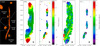 |
Fig. 1. HST/WFC3 F160W near-infrared image (left panel), [O II] (middle left panel) and CO (middle panel) emission line velocity maps, and [O II] (middle right panel) and CO (right panel) velocity dispersion maps of the Cosmic Snake in the image plane. The PSF of 0.51″ of the kinematic maps is shown as a gray circle in the bottom right corner. The black contours indicate velocities of 30 and 90 km s−1. The critical line from the lensing model is shown in white in the left panel. The HST image and kinematic maps are at the same scale. The velocity dispersion maps are corrected for the instrumental broadening, but uncorrected for beam-smearing. |
A521 is a typical disk galaxy that shows clear spiral arms (Richard et al. 2010; Patrício et al. 2018). This galaxy is lensed into three counter-images of the same galaxy. The first counter-image is located in the northeast (see Fig. 2) and shows a spiral galaxy that is barely distorted, with two clear spiral arms. The two other counter-images are more distorted and elongated due to higher magnifications and are located to the west. The second counter-image in the northeast region shows the same first spiral arm, and in the south region, a second spiral arm. The third image is smaller and represents only the last few spaxels in the southwest of the kinematic maps. In contrast to the Cosmic Snake, where we detect the CO emission only in the center of the galaxy, here the CO traces the spiral arms. Again, in the CO kinematic maps (right panels of Fig. 2), we clearly distinguish the east part (which includes the first counter-image) and the west part (which includes the second and third counter-images).
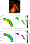 |
Fig. 2. HST/WFC3 F160W near-infrared image (top panel), [O II] emission line velocity map (middle left), CO line velocity map (middle right), [O II] emission line velocity dispersion map (bottom left) and CO line velocity dispersion map (bottom right) of A521 in the image plane. The PSF of 0.69″ of the kinematic maps is shown as a gray circle in the bottom left corner. Both velocity dispersion maps are corrected for the instrumental broadening, but uncorrected for beam-smearing. The critical line from the lensing model is shown in white in the top panel. The HST image and kinematic maps are at the same scale. |
The main properties of the Cosmic Snake and A521, including their stellar mass, M⋆, star formation rate, SFR, and redshift z, are presented in Table 1. The two galaxies show several star-forming clumps (see Cava et al. 2018 for the Cosmic Snake) and lie on the main sequence of star-forming galaxies at this redshift (see Fig. 3 in Patrício et al. 2018). They are also included in the sample studied by Patrício et al. (2018), who measured inclinations of 70° and 72° from kinematic models for the Cosmic Snake and A521, respectively. Using a model that takes the lensing and beam-smearing effects into account, they found υrot/σ0 ratios of 5.1 ± 3.6 and 2.1 ± 0.8 for the Cosmic Snake and A521, respectively, which are typical at z ∼ 1 (e.g., Wisnioski et al. 2015). This suggests that these two galaxies are disks that are dominated by rotation.
Galaxy properties.
3. Observations, data reduction, and analysis
3.1. [O II] observations with MUSE/VLT
The observations, data reduction, and emission line measurements are described in Patrício et al. (2018). The observations were seeing-limited for the Cosmic Snake, and A521 was observed with adaptive optics. The point spread functions (PSF) obtained during the observations were 0.51″ and 0.57″, respectively (see Table 1).
Patrício et al. (2018) derived the velocity field and velocity dispersion maps of the Cosmic Snake and A521 by fitting the [O II]λ3726, 3729 Å emission lines with Gaussian profiles in the image plane using the CAMEL code (Epinat et al. 2010). They used a Voronoi binning when the signal-to-noise ratio was lower than 5 in a spaxel in A521 (Cappellari & Copin 2003). The A521 maps have been slightly smoothed during this process. Therefore, the final PSFs of the Cosmic Snake and A521 are ∼0.51″ and ∼0.69″, respectively. The spectral resolution of MUSE is ∼50 km s−1.
3.2. CO observations with ALMA
Observations of the Cosmic Snake were carried out in Cycle 3 (project 2013.1.01330.S) and were performed in the extended C38-5 configuration with the maximum baseline of 1.6 km and 38 of the 12-m antennae. The total on-source integration time was of 52.3 min in band 6. We observed the CO(4-3) emission line at the observed frequency of 226.44 GHz, which corresponds to a redshift of z = 1.036. A521 was observed in Cycle 4 (project 2016.1.00643.S) using the C40-6 configuration with the maximum baseline of 3.1 km and 41 of the 12-m antennae. Similarly, the observations were carried out in band 6 to detect the CO(4-3) emission line at an observed frequency of 225.66 GHz, corresponding to a redshift of z = 1.043, with an on-source time of 89.0 min. The spectral resolution was tuned to 7.8125 MHz (∼10.3 km s−1) for both galaxies.
The data reduction was performed with the standard automated reduction procedure from the pipeline of the Common Astronomy Software Application (CASA) package (McMullin et al. 2007). To image the CO(4-3) line, we used the Briggs weighting and the robust factor of 0.5, which is a good compromise between resolution and sensitivity. We cleaned all channels interactively with the clean routine in CASA until convergence. To perform the cleaning, we used a custom mask for which we ensured that the CO emission of all the channels was included. We then applied the primary beam correction. The final synthesized beam size is 0.22″ × 0.18″ with a position angle of +85° for the Cosmic Snake and 0.20″ × 0.17″ at −71° for A521. We reach an rms of 0.29 mJy beam−1 and 0.34 mJy beam−1 per 7.8125 MHz channel for the Cosmic Snake and A521, respectively.
The data cubes for the Cosmic Snake and A521 were smoothed with the imsmooth routine in CASA to a spatial resolution of 0.51″ and 0.69″, respectively, to obtain the same final spatial resolution as for the MUSE data. We finally used the immoments routine in CASA to obtain the CO(4-3) moment maps, and applied a 3σ threshold parameter above the noise level when the first (velocity) and second (velocity dispersion) moment maps were produced.
3.3. Gravitational lens modeling
The two galaxies presented in this work are highly magnified and have multiple images, therefore we used a lensing model to recover the physical galactocentric radius corrected for the lensing magnification. We used the lensing models that were presented in detail in Cava et al. (2018) and Richard et al. (2010) for the Cosmic Snake and A521, respectively, which were based on multiple images identified in HST imaging. Lenstool was used to constrain the mass distribution and to optimize the models for these two galaxies using their multiple images. Uncertainties on the magnification vary between 10 and 20%. The lens model achieves an rms precision of 0.15″ and 0.23″ between the predicted and observed locations of the strong lensing constraints as measured in the image plane of the Cosmic Snake and A521 arcs, respectively.
4. Comparison of the molecular and ionized gas kinematics
Figures 1 and 2 show the observed velocity and velocity dispersion maps of the Cosmic Snake and A521 in the image plane at a spatial resolution of ∼0.51″ and ∼0.69″, respectively, with the HST/WFC3 F160W images (program #15435). The [O II] and CO(4-3) kinematic maps were measured in the galaxy rest-frame using the redshifts indicated in Table 1. The velocity dispersion maps were corrected for their corresponding instrumental broadening, σinstr, using the following relation:
 (1)
(1)
To measure the rotation curves and velocity dispersion profiles, we constructed concentric annuli in the source plane. The width of these annuli was chosen to be slightly larger than the physical spaxel size. We then projected them in the image plane with spaxels of the same size as the ALMA and MUSE data. We thus obtained the physical distance to the center in the source plane for every spaxel. We defined the major axis as the line following the direction of the steepest velocity gradient using the maximum and minimum values in each annulus on the velocity map. These major axes correspond well those derived in Patrício et al. (2018). The rotation curves and velocity dispersion profiles were measured directly from the velocity and velocity dispersion maps in the image plane by taking an aperture corresponding to the PSF along the major axis. This method was verified using a simulated galaxy in the source plane and projected in the image plane. We accurately recovered the kinematics (with an error smaller than 10%). To measure the final rotation curves, we took only the mean values of the positive side of the rotation curves of two counter-images for each galaxy that showed the highest visible fraction of the source galaxy: the north and south parts of the Cosmic Snake, and the northeast part (first image) and the east image of the west part (second image) of A521. We did not include negative velocities because less than 20% of the negative velocities from the background galaxies are lensed (see Sect. 2).
Figures 3 and 4 present the observed rotation curves, uncorrected for the inclination, and velocity dispersion profiles, uncorrected for the beam-smearing, of the CO and [O II] emission lines of the Cosmic Snake and A521, respectively. The solid line represents the average values obtained from the two counter-images in both cases. The error bars were determined from the velocity measurement in the two counter-images for the two galaxies. The profiles of the Cosmic Snake and A521 have an average spatial resolution of few hundred parsec (∼500 pc) and few kiloparsecs (∼2 − 3 kpc), respectively. Because the major axis of A521 is perpendicular to the stretching direction, the spatial resolution we obtained is not as high as for the Cosmic Snake.
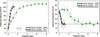 |
Fig. 3. Observed velocity (left panel) and velocity dispersion profiles (right panel) of the Cosmic Snake from the [O II] emission line (in green) and CO(4-3) line (in black). The solid line is the average rotation curve of the two counter-images. The curves are extracted from the observed data in the image plane, uncorrected for beam-smearing or inclination. The data cubes for CO and [O II] were convolved to the same spatial resolution of 0.51″ (∼500 pc on average). The two dashed lines indicate the intrinsic velocity dispersion of 19.5 ± 6 km s−1 and 18.5 ± 7 km s−1 measured from the [O II] (in green) and CO (in black) velocity dispersion maps at large radii (R > Re when possible), respectively. |
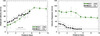 |
Fig. 4. Observed velocity (left panel) and velocity dispersion profiles (right panel) of A521 from the [O II] emission line (in green) and CO(4-3) line (in black). The solid line is the average rotation curve of the two counter-images. The curves are extracted from the observed data in the image plane, uncorrected for beam-smearing or inclination. The data cubes for CO and [O II] were convolved to the same spatial resolution of 0.69″ (∼2 − 3 kpc on average). The two dashed lines indicate the intrinsic velocity dispersion of 54 ± 11 km s−1 and 11 ± 8 km s−1 measured from the [O II] (in green) and CO (in black) velocity dispersion maps at large radii (R > Re when possible), respectively. |
Figure 3 shows a clear difference between the molecular and ionized gas rotation curves of the Cosmic Snake. The molecular gas curve is steeper and reaches the maximum rotation velocity at a smaller radius from the center than the ionized gas curve. On the other hand, A521 does not show a difference between the CO and [O II] rotation curves (Fig. 4).
We determined the intrinsic velocity dispersion by directly measuring the velocity dispersion maps along the major axis in the outer regions (at radii larger than the effective radius, Re, when possible) where the rotation curve is flat and beam-smearing is negligible (e.g., Förster Schreiber et al. 2009; Girard et al. 2018a). We obtained a similar intrinsic velocity dispersion of 18.5 ± 7 km s−1 and 19.5 ± 6 km s−1 for the molecular and ionized gas, respectively, for the Cosmic Snake. For A521, we find different values of 11 ± 8 km s−1 and 54 ± 11 km s−1, respectively. Patrício et al. (2018) used a different method to estimate the intrinsic velocity dispersion: they corrected in quadrature the beam-smearing determined from the modeled velocity dispersion. They obtained values of 44 ± 31 km s−1 and 63 ± 23 km s−1 for the ionized gas intrinsic velocity dispersion in the Cosmic Snake and A521, respectively.
5. Modeled gas rotation curves
We focus here on how the geometrical effects, such as the effective radius and thickness of the gas disk, can influence the shape of the rotation curve. We also study the differences this causes in the rotation curves of distinct gas tracers.
5.1. Model
In order to build a realistic and self-consistent rotation curve model, that includes a disk of stars and gas, and possibly a bulge or dark matter component, we chose to describe the various mass components by analytical density-potential pairs, and then performed a numerical simulation of gas particles in the resulting potential. This allowed us more flexibility to study the various gas tracers that can then sample the same rotation curve with different weights. We represented the stellar and gaseous disks by Miyamoto–Nagai disks (Miyamoto & Nagai 1975), with masses, radial scales, and heights corresponding to the observations. For the simulation, we typically distributed one million particles according to the analytical distributions of the gas disk components, with their relative effective radii and scale heights. The gas particles were distributed in nearly circular orbits, in equilibrium with the total potential, with a velocity distribution corresponding to the Toomre Q-parameter. The ratio between tangential and radial velocity dispersion was taken from the epicyclic theory (e.g., Toomre 1964).
To reconstruct a rotation curve from the particle positions and velocities, we assumed an inclination and then produced a 2D velocity map by taking the average velocity of the particles along the line of sight in each spatial element. The velocity map can be adjusted to the same average physical spatial resolution as the observations (in kiloparsec). Afterwards, we extracted the rotation curve in a similar way as an observed velocity map by measuring the values along the major axis.
We first investigated the general effect of the effective radius and scale height of a gas disk, Rgas and Hgas, on the rotation curve for a model that only includes a stellar disk and a single gas disk. We neglected the dark matter because we concentrated on the baryons in the center of a typical relatively massive galaxy. We also neglected the bulge because its effect on the molecular and ionized gas kinematics are negligible. This model used six fixed parameters for the stellar and gas disks: the stellar mass, M⋆, the stellar disk effective radius, R⋆, the stellar disk scale height, H⋆, the gas mass, Mgas(or the gas fraction, fgas, where fgas = Mgas/(Mgas + M⋆)), the Toomre stability parameter, Q, and the inclination, i. For the stellar mass and gas fraction, we used values similar to the molecular gas disks of the Cosmic Snake and A521 to represent a typical galaxy at high redshift with M⋆ = 3 × 10¹⁰ M⊙, fgas = 0.2, and an inclination of i = 70°. For the stellar disk, we adopted values established in the literature for nearby galaxies with R⋆ = 4.0 kpc and H⋆ = 0.5 kpc (e.g., van der Kruit & Freeman 2011; Ma et al. 2017). Finally, we fixed the Toomre Q-parameter to a value of 1, which represents a quasi-stable disk for a thin gas disk (e.g., Genzel et al. 2011).
Figure 5 shows the rotation curves obtained for an effective radius of the gas disk of 0.5 kpc (green), 1 kpc (orange), 5 kpc (blue), and 10 kpc (magenta). The upper and lower boundaries (taking absolute values) of the plotted rotation curves for the four effective radii correspond to a gas disk height of 50 pc and 3 kpc, respectively. A disk height of 50 pc is typically observed for a molecular gas disk in the local Universe (e.g., Glazebrook 2013). We adopted a maximum value of 3 kpc for the disk height, because the average and maximum disk height values reported for high-redshift galaxies are ∼0.63 kpc and ∼2.5 kpc, respectively (Elmegreen et al. 2017).
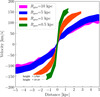 |
Fig. 5. Effect of the gas disk effective radius, Rgas, and height, Hgas, on the rotation curve. The values of the gas disk effective radius are 0.5 kpc (green), 1 kpc (orange), 5 kpc (blue), and 10 kpc (pink). The upper and lower boundaries (taking the absolute values) of each colored curve represent a disk height of 50 pc and 3 kpc, respectively. The other parameters are fixed to M⋆ = 3 × 10¹⁰ M⊙, R⋆ = 4.0 kpc, H⋆ = 0.5 kpc, fgas = 0.2, i = 70°, and Q = 1. |
The effective radius strongly affects the shape of the rotation curve. The rotation curve of a disk with a smaller radius reaches the maximum rotation velocity at a smaller radius than a more extended disk, meaning that the smaller the effective radius, the steeper the rotation curve. The thickness of the gas disk also affects the rotation curve. A thicker disk smoothens the rotation curve, such that the curve becomes flatter with increasing thickness. The effect of the thickness is less pronounced than the effect of the effective radius.
5.2. Effect of the thickness and inclination on the spatial resolution
The presence of a thick disk when a galaxy is strongly inclined limits the spatial resolution we can obtain on the observed rotation curve. The highest spatial resolution that can be obtained for an inclined thick disk can be described by
 (2)
(2)
where H is the height of the disk, and i is the inclination of the galaxy. This means that a galaxy with a thick disk and a high inclination could have a lower spatial resolution than the resolution expected from the observations. We investigated the effect of the spatial resolution on the rotation curve using the model described in Sect. 5.1, with Rgas = 1 kpc and Hgas = 1 kpc. We convolved the 2D velocity maps of this model for an inclination of i = 70° and i = 80° to derive their velocity maps at the spatial resolution determined by Eq. (2) with their corresponding inclination and gas height. We then extracted the respective rotation curves. Figure 6 shows the simulated rotation curves for an inclination of i = 70° (orange) and i = 80° (blue) together with the rotation curves smoothed due to the lower spatial resolution. The spatial resolution effect is much stronger for an inclination of i = 80°. Therefore, a high inclination also strongly smoothens the rotation curve when a thick disk is present (> 1 kpc).
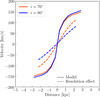 |
Fig. 6. Effect of the inclination on the rotation curve due to the spatial resolution. The solid curves represent the rotation curves that were simulated using the same parameters as in Fig. 5, with Rgas = 1 kpc and Hgas = 1 kpc for an inclination of i = 70° (orange) and i = 80° (blue). The dashed lines present the two models smoothed to the spatial resolution determined by Eq. (2) with their corresponding inclinations and Hgas = 1 kpc. |
6. Analysis of two lensed z ∼ 1 galaxies
In this section we investigate if the difference observed between the rotation curves and velocity dispersion values of the molecular and ionized gas can be explained by geometrical effects in the Cosmic Snake and A521.
6.1. Cosmic Snake
To build a realistic model that represents the Cosmic Snake, we distinguished two gas disks, one for the molecular component, and the second for the ionized gas component. Because we only observe the baryon-dominated central parts of a relatively massive galaxy, the contribution from the dark matter is negligible. The bulge component was also neglected because it does not strongly affect the gas kinematics.
For the stellar disk, the stellar mass was taken from the work of Cava et al. (2018). We measured a stellar effective radius of R⋆ = 3.8 ± 0.7 kpc from the radial mass profile, and we adopted a stellar scale height typical of nearby disk galaxies with H⋆ ∼ 0.5 kpc (e.g., van der Kruit & Freeman 2011; Ma et al. 2017). From the CO luminosity profile, we measured the molecular effective radius to be  kpc and estimated the molecular height to be Hmol < 450 pc. We chose to fix the height to 100 pc because using a value between 50 pc and 450 pc does not strongly influence the results (see Fig. 5). The mass of the molecular gas disk was determined from the gas fraction of fgas = 0.20 ± 0.03 obtained in Dessauges-Zavadsky et al. (2019). We estimated the ionized gas mass to be (2.0 ± 0.2)×107 M⊙ from the absolute B magnitude following the relation of López-Sánchez (2010). This mass is very low in comparison to the total mass of the galaxy (fion ≪ 1%) and does not contribute to the potential of the galaxy. Our results are therefore not sensitive to this estimate. We derived an effective radius of
  kpc for the ionized gas disk from the radial [O II] profile. We varied the ionized gas height between 1 and 3 kpc, because it does not affect the potential of the galaxy. Finally, the (Toomre 1964) stability parameter Q was directly measured using the relation
 (3)
(3)
where the instrinsic velocity dispersion is σ0 ∼ 19.5 ± 6 km s−1 (from this work), the rotation velocity corrected for the inclination is υrot = 225 ± 1 km s−1 (Patrício et al. 2018), and the gas fraction is fgas = 0.20 ± 0.03 (Dessauges-Zavadsky et al. 2019). We thus obtain Q ∼ 0.6 for both the molecular and ionized gas disks, because they show a similar velocity dispersion. We assumed an inclination, i, of 70 ° ±1° for the molecular and ionized gas disk according to the kinematic model obtained by Patrício et al. (2018) for this galaxy. A difference in inclination between these two disks is not expected because the ionized gas results from the stars that form inside the molecular clouds. The parameters are listed in Table 2.
Parameters of the model for the Cosmic Snake.
Figure 7 shows the simulated molecular and ionized gas rotation curves together with the observed rotation curves from the CO and [O II] of the Cosmic Snake. The simulations are in very good agreement with the observed rotation curves. The rotation curves of the molecular and ionized gas are well reproduced by disks with different radii and heights. This means that the molecular gas disk of the Cosmic Snake is likely more concentrated in the center of the galaxy and probably has a thinner disk than the ionized gas disk. Galaxies with a thin molecular disk are also typically observed in the local Universe (e.g., Glazebrook 2013). Some observations of local galaxies also reveal that the molecular gas is more concentrated in the center of several galaxies (e.g., Wong & Blitz 2002; Leroy et al. 2008).
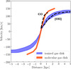 |
Fig. 7. Rotation curves obtained in the simulated mass distribution corresponding to the parameters listed in Table 2, with two tracers: the molecular and ionized components. The results from the simulation for the molecular and ionized gas disks are shown in orange and in blue, respectively. The upper and lower boundaries of the ionized gas disk (taking the absolute values) represent a height of 1 kpc and 3 kpc, respectively. The dashed black lines indicate the observed CO and [O II] rotation curves of the Cosmic Snake. |
This is in agreement with the relation relation of the radius and disk height to the rotation velocity and velocity dispersion of the disk (e.g., Genzel et al. 2011; White et al. 2017):
 (4)
(4)
where R and H are the radius and height of the disk. In the Cosmic Snake, we obtain a similar intrinsic velocity dispersion and rotation velocity in the ionized and molecular gas disks, meaning that both disks have similar υrot/σ0 ratios and radius-to-height ratios, R/H. This is consistent with lower values for both the radius and height of the molecular gas disk compared to the ionized gas disk.
With this model, we can also test how an ionized gas thick disk degrades the spatial resolution along the line of sight in the Cosmic Snake and how it affects the shape of the rotation curve. We convolved the 2D ionized gas velocity maps with an ionized gas disk height, Hion, of 1 kpc, 2 kpc, and 3 kpc to create velocity maps at the spatial resolution determined by Eq. (2) with their corresponding height and at the inclination of the Cosmic Snake (i = 70°). We then extracted the respective rotation curves. Figure 8 shows the simulated ionized gas rotation curves for an ionized gas disk height of 1 kpc (orange), 2 kpc (blue), and 3 kpc (pink) together with the rotation curves smoothed due to the lower spatial resolution. First, an ionized gas height of ∼1 kpc fits the observations relatively well. We also find that the spatial resolution effect increases for a thicker disk of Hion = 2 kpc and Hion = 3 kpc. This means that the lower spatial resolution caused by a thick disk plays a major role in shaping the ionized gas rotation curve of the Cosmic Snake because of the high inclination of i = 70° of this galaxy. As seen in Sect. 5.2, a thick disk affects the shape of the rotation curve even more as a result of this effect in the case of a more highly inclined disk.
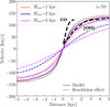 |
Fig. 8. Effect of the ionized gas disk height on the rotation curve due to the spatial resolution for the Cosmic Snake. The colored solid curves are the rotation curves simulated in the mass distribution corresponding to the parameters listed in Table 2 with an ionized disk height of 1 kpc (orange), 2 kpc (blue) and 3 kpc (pink). The dashed colored curves represent the curves smoothed to the spatial resolution determined by Eq. (2) with their corresponding disk height. The inclination has been fixed to i = 70°, which is the inclination of the Cosmic Snake. The dashed black lines indicate the observed CO and [O II] rotation curves of the Cosmic Snake. |
6.2. A521
In contrast to the Cosmic Snake, the [O II] and CO rotation curves are in good agreement in the galaxy A521, similar to the result of Übler et al. (2018). However, when we ran simulations at the spatial resolution observed in A521 (∼2 − 3 kpc), we obtained that the difference between the [O II] and CO rotation curves observed in the Cosmic Snake at a spatial resolution of few hundred parsec (∼500 pc) is much less pronounced. The lack of spatial resolution can easily prevent us from seeing a difference between two rotation curves. However, because the CO emission in A521 is also much more radially extended (Rmol = 5.8 ± 1.0 kpc) than [O II] (Rion = 6.5 ± 1.2 kpc), a molecular gas rotation curve as steep as for the Cosmic Snake is not expected according to Fig. 5.
We also observe a very different intrinsic velocity dispersion for the molecular and ionized gas in this galaxy with values of 11 ± 8 km s−1 and 54 ± 11 km s−1, respectively. Übler et al. (2018) found a similar value of ∼15 − 30 km s−1 from the molecular and ionized gas in their galaxy at z ∼ 1.4. Values of ∼10 − 20 km s−1 and ∼20 − 40 km s−1 for the molecular and ionized gas, respectively, have been found by Cortese et al. (2017) at z ∼ 0.2, which are very similar to what is found for typical spiral galaxies at z ∼ 0 (e.g., Epinat et al. 2010; Levy et al. 2018). The velocity dispersion of the molecular gas of A521 is similar to galaxies in the local Universe. However, the velocity dispersion from the ionized gas of A521 is higher than galaxies in the local Universe, but this is also observed for high-redshift galaxies in many studies (e.g., Förster Schreiber et al. 2009; Wisnioski et al. 2015; Johnson et al. 2018; Girard et al. 2018a). This could mean that the ionized gas disk is more turbulent than the molecular disk and might indicate the presence of a thick disk in this galaxy. Given also the high inclination of 72° in A521, a difference in thickness of the molecular and ionized gas disks is expected to cause a difference between the two rotation curves according to Figs. 6 and 8. It is therefore possible that the molecular gas has an intrinsically steeper rotation curve, but that the available spatial resolution does not resolve it.
7. Conclusions
We have presented the molecular gas kinematics from ALMA CO(4-3) observations of two highly magnified galaxies at z ∼ 1 and compared it with the [O II] kinematics obtained with MUSE/VLT (Patrício et al. 2018). These two galaxies, called the Cosmic Snake and A521, are located behind the clusters MACS J1206.2−0847 and Abell 0521.
We derived the observed rotation curves and velocity dispersion profiles in the image plane for both galaxies. For the Cosmic Snake, where we obtain a spatial resolution of only a few hundred parsec on the major axis, we observe a difference between the molecular and ionized gas rotation curves in the inner part of the galaxy (0 − 2 kpc). The molecular gas curve is steeper than the ionized gas curve. In A521, the molecular and ionized gas rotation curves agree, but the spatial resolution is only a few kiloparsec on the major axis.
Using simulations, we studied the effect of the effective radius and thickness of the gas disk on the observed rotation curve and find that a more extended and thicker disk smoothens the curve. We also find that a thick disk (Hgas > 1 kpc), when the galaxy is strongly inclined (i > 70°), can smoothen the rotation curve because it degrades the spatial resolution along the line of sight.
We reproduced the observed rotation curves of the Cosmic Snake using a model that includes a stellar disk and two gas disks, with a molecular gas disk that is more massive and more radially and vertically concentrated than the ionized gas disk. The model suggests a thick ionized gas disk with a scale height of Hion ∼ 1 kpc. We measure an intrinsic velocity dispersion of 18.5 ± 7 km s−1 and 19.5 ± 6 km s−1 for the molecular and ionized gas of the Cosmic Snake. Similar values of the maximum rotation velocity and intrinsic velocity dispersion agree with a molecular gas disk that is more concentrated in the center of the galaxy and thinner than the ionized gas disk. For A521, we obtain values of 11 ± 8 km s−1 and 54 ± 11 km s−1 for the velocity dispersion, with a higher value for the ionized gas. This difference could indicate the presence of a thick and turbulent ionized gas disk.
Taken together, these two galaxies highlight the diversity in the kinematics observed at z ∼ 1. The galaxy kinematics reflect the different spatial distribution of the molecular and ionized gas disks and confirm the presence of thick ionized gas disks at this epoch. These thick ionized gas disks are believed to be the result of the turbulence in the gas of young gas-rich galaxies (e.g., Förster Schreiber et al. 2009). A thinner and less radially extended molecular gas disk could also indicate that the formation of the molecular gas is limited to the central regions in some galaxies because of the low pressure or lack of metals outside the midplane and center of the galaxy (e.g., Wong & Blitz 2002).
Acknowledgments
This work was supported by the Swiss National Science Foundation. MG is grateful to the Fonds de recherche du Québec – Nature et Technologies (FRQNT) for financial support. JR acknowledges support from the ERC Starting Grant 336736-CALENDS. Based on observations made with the NASA/ESA Hubble Space Telescope, obtained from the Data Archive at the Space Telescope Science Institute, which is operated by the Association of Universities for Research in Astronomy, Inc., under NASA contract NAS 5-26555. These observations are associated with program #15435.
References
- Barro, G., Kriek, M., Pérez-González, P. G., et al. 2017, ApJ, 851, L40 [NASA ADS] [CrossRef] [Google Scholar]
- Bland-Hawthorn, J., & Gerhard, O. 2016, ARA&A, 54, 529 [NASA ADS] [CrossRef] [EDP Sciences] [Google Scholar]
- Bosma, A., & van der Kruit, P. C. 1979, A&A, 79, 281 [NASA ADS] [Google Scholar]
- Calistro Rivera, G., & Hodge, J. 2018, The Messenger, 173, 33 [NASA ADS] [Google Scholar]
- Cappellari, M., & Copin, Y. 2003, MNRAS, 342, 345 [NASA ADS] [CrossRef] [Google Scholar]
- Carignan, C., Chemin, L., Huchtmeier, W. K., & Lockman, F. J. 2006, ApJ, 641, L109 [NASA ADS] [CrossRef] [Google Scholar]
- Cava, A., Schaerer, D., Richard, J., et al. 2018, Nat. Astron., 2, 76 [Google Scholar]
- Cortese, L., Catinella, B., & Janowiecki, S. 2017, ApJ, 848, L7 [NASA ADS] [CrossRef] [Google Scholar]
- de Blok, W. J. G., Walter, F., Brinks, E., et al. 2008, AJ, 136, 2648 [NASA ADS] [CrossRef] [Google Scholar]
- Dessauges-Zavadsky, M., Richard, J., Combes, F., et al. 2019, Nat. Astron., 436 [Google Scholar]
- Elmegreen, B. G., Elmegreen, D. M., Tompkins, B., & Jenks, L. G. 2017, ApJ, 847, 14 [NASA ADS] [CrossRef] [Google Scholar]
- Epinat, B., Amram, P., Balkowski, C., & Marcelin, M. 2010, MNRAS, 401, 2113 [NASA ADS] [CrossRef] [Google Scholar]
- Ford, Jr., W. K., Rubin, V. C., & Roberts, M. S. 1971, AJ, 76, 22 [NASA ADS] [CrossRef] [Google Scholar]
- Förster Schreiber, N. M., Genzel, R., Bouché, N., et al. 2009, ApJ, 706, 1364 [NASA ADS] [CrossRef] [Google Scholar]
- Frank, B. S., de Blok, W. J. G., Walter, F., Leroy, A., & Carignan, C. 2016, AJ, 151, 94 [NASA ADS] [CrossRef] [Google Scholar]
- Genzel, R., Newman, S., Jones, T., et al. 2011, ApJ, 733, 101 [NASA ADS] [CrossRef] [Google Scholar]
- Girard, M., Dessauges-Zavadsky, M., Schaerer, D., et al. 2018a, A&A, 613, A72 [NASA ADS] [CrossRef] [EDP Sciences] [Google Scholar]
- Girard, M., Dessauges-Zavadsky, M., Schaerer, D., et al. 2018b, A&A, 619, A15 [NASA ADS] [CrossRef] [EDP Sciences] [Google Scholar]
- Glazebrook, K. 2013, PASA, 30, 56 [CrossRef] [Google Scholar]
- Guérou, A., Krajnović, D., Epinat, B., et al. 2017, A&A, 608, A5 [NASA ADS] [CrossRef] [EDP Sciences] [Google Scholar]
- Johnson, H. L., Harrison, C. M., Swinbank, A. M., et al. 2018, MNRAS, 474, 5076 [NASA ADS] [CrossRef] [Google Scholar]
- Jones, T. A., Swinbank, A. M., Ellis, R. S., Richard, J., & Stark, D. P. 2010, MNRAS, 404, 1247 [NASA ADS] [Google Scholar]
- Leethochawalit, N., Jones, T. A., Ellis, R. S., et al. 2016, ApJ, 820, 84 [NASA ADS] [CrossRef] [Google Scholar]
- Leroy, A. K., Walter, F., Brinks, E., et al. 2008, AJ, 136, 2782 [NASA ADS] [CrossRef] [Google Scholar]
- Levy, R. C., Bolatto, A. D., Teuben, P., et al. 2018, ApJ, 860, 92 [NASA ADS] [CrossRef] [Google Scholar]
- Livermore, R. C., Jones, T. A., Richard, J., et al. 2015, MNRAS, 450, 1812 [NASA ADS] [CrossRef] [Google Scholar]
- López-Sánchez, Á. R. 2010, A&A, 521, A63 [NASA ADS] [CrossRef] [EDP Sciences] [Google Scholar]
- Ma, X., Hopkins, P. F., Wetzel, A. R., et al. 2017, MNRAS, 467, 2430 [Google Scholar]
- Mason, C. A., Treu, T., Fontana, A., et al. 2017, ApJ, 838, 14 [NASA ADS] [CrossRef] [Google Scholar]
- Matthee, J., Sobral, D., Boone, F., et al. 2017, ApJ, 851, 145 [NASA ADS] [CrossRef] [Google Scholar]
- McMullin, J. P., Waters, B., Schiebel, D., Young, W., & Golap, K. 2007, in Astronomical Data Analysis Software and Systems XVI, eds. R. A. Shaw, F. Hill, & D. J. Bell, ASP Conf. Ser., 376, 127 [Google Scholar]
- Miyamoto, M., & Nagai, R. 1975, PASJ, 27, 533 [NASA ADS] [Google Scholar]
- Olivares, V., Treister, E., Privon, G. C., et al. 2016, ApJ, 827, 57 [NASA ADS] [CrossRef] [Google Scholar]
- Patrício, V., Richard, J., Carton, D., et al. 2018, MNRAS, 477, 18 [NASA ADS] [CrossRef] [Google Scholar]
- Richard, J., Smith, G. P., Kneib, J.-P., et al. 2010, MNRAS, 404, 325 [NASA ADS] [Google Scholar]
- Richards, E. E., van Zee, L., Barnes, K. L., et al. 2016, MNRAS, 460, 689 [NASA ADS] [CrossRef] [Google Scholar]
- Rubin, V. C. 1983, Sci. Am., 248, 96 [NASA ADS] [CrossRef] [Google Scholar]
- Salpeter, E. E. 1955, ApJ, 121, 161 [Google Scholar]
- Schmidt, M. 1957, Bull. Astron. Inst. Neth., 14, 17 [NASA ADS] [Google Scholar]
- Smit, R., Bouwens, R. J., Carniani, S., et al. 2018, Nature, 553, 178 [NASA ADS] [CrossRef] [Google Scholar]
- Sofue, Y. 1996, ApJ, 458, 120 [NASA ADS] [CrossRef] [Google Scholar]
- Sofue, Y., & Rubin, V. 2001, ARA&A, 39, 137 [NASA ADS] [CrossRef] [Google Scholar]
- Sofue, Y., Tomita, A., Honma, M., & Tutui, Y. 1999, PASJ, 51, 737 [NASA ADS] [CrossRef] [Google Scholar]
- Sorai, K., Nakai, N., Kuno, N., Nishiyama, K., & Hasegawa, T. 2000, PASJ, 52, 785 [NASA ADS] [CrossRef] [Google Scholar]
- Stott, J. P., Swinbank, A. M., Johnson, H. L., et al. 2016, MNRAS, 457, 1888 [NASA ADS] [CrossRef] [Google Scholar]
- Swinbank, A. M., Harrison, C. M., Trayford, J., et al. 2017, MNRAS, 467, 3140 [NASA ADS] [Google Scholar]
- Swinbank, A. M., Papadopoulos, P. P., Cox, P., et al. 2011, ApJ, 742, 11 [NASA ADS] [CrossRef] [Google Scholar]
- Toomre, A. 1964, ApJ, 139, 1217 [Google Scholar]
- Turner, O. J., Cirasuolo, M., Harrison, C. M., et al. 2017, MNRAS, 471, 1280 [NASA ADS] [CrossRef] [Google Scholar]
- Übler, H., Genzel, R., Tacconi, L. J., et al. 2018, ApJ, 854, L24 [NASA ADS] [CrossRef] [Google Scholar]
- Übler, H., Genzel, R., Wisnioski, E., et al. 2019, ApJ, 880, 48 [NASA ADS] [CrossRef] [Google Scholar]
- van de Hulst, H. C., Raimond, E., & van Woerden, H. 1957, Bull. Astron. Inst. Neth., 14, 1 [NASA ADS] [Google Scholar]
- van der Kruit, P. C., & Allen, R. J. 1978, ARA&A, 16, 103 [NASA ADS] [CrossRef] [Google Scholar]
- van der Kruit, P. C., & Freeman, K. C. 2011, ARA&A, 49, 301 [NASA ADS] [CrossRef] [Google Scholar]
- White, H. A., Fisher, D. B., Murray, N., et al. 2017, ApJ, 846, 35 [NASA ADS] [CrossRef] [Google Scholar]
- Wisnioski, E., Förster Schreiber, N. M., Wuyts, S., et al. 2015, ApJ, 799, 209 [NASA ADS] [CrossRef] [Google Scholar]
- Wong, T., & Blitz, L. 2002, ApJ, 569, 157 [NASA ADS] [CrossRef] [Google Scholar]
All Tables
All Figures
|
Fig. 1. HST/WFC3 F160W near-infrared image (left panel), [O II] (middle left panel) and CO (middle panel) emission line velocity maps, and [O II] (middle right panel) and CO (right panel) velocity dispersion maps of the Cosmic Snake in the image plane. The PSF of 0.51″ of the kinematic maps is shown as a gray circle in the bottom right corner. The black contours indicate velocities of 30 and 90 km s−1. The critical line from the lensing model is shown in white in the left panel. The HST image and kinematic maps are at the same scale. The velocity dispersion maps are corrected for the instrumental broadening, but uncorrected for beam-smearing. |
| In the text | |
|
Fig. 2. HST/WFC3 F160W near-infrared image (top panel), [O II] emission line velocity map (middle left), CO line velocity map (middle right), [O II] emission line velocity dispersion map (bottom left) and CO line velocity dispersion map (bottom right) of A521 in the image plane. The PSF of 0.69″ of the kinematic maps is shown as a gray circle in the bottom left corner. Both velocity dispersion maps are corrected for the instrumental broadening, but uncorrected for beam-smearing. The critical line from the lensing model is shown in white in the top panel. The HST image and kinematic maps are at the same scale. |
| In the text | |
|
Fig. 3. Observed velocity (left panel) and velocity dispersion profiles (right panel) of the Cosmic Snake from the [O II] emission line (in green) and CO(4-3) line (in black). The solid line is the average rotation curve of the two counter-images. The curves are extracted from the observed data in the image plane, uncorrected for beam-smearing or inclination. The data cubes for CO and [O II] were convolved to the same spatial resolution of 0.51″ (∼500 pc on average). The two dashed lines indicate the intrinsic velocity dispersion of 19.5 ± 6 km s−1 and 18.5 ± 7 km s−1 measured from the [O II] (in green) and CO (in black) velocity dispersion maps at large radii (R > Re when possible), respectively. |
| In the text | |
|
Fig. 4. Observed velocity (left panel) and velocity dispersion profiles (right panel) of A521 from the [O II] emission line (in green) and CO(4-3) line (in black). The solid line is the average rotation curve of the two counter-images. The curves are extracted from the observed data in the image plane, uncorrected for beam-smearing or inclination. The data cubes for CO and [O II] were convolved to the same spatial resolution of 0.69″ (∼2 − 3 kpc on average). The two dashed lines indicate the intrinsic velocity dispersion of 54 ± 11 km s−1 and 11 ± 8 km s−1 measured from the [O II] (in green) and CO (in black) velocity dispersion maps at large radii (R > Re when possible), respectively. |
| In the text | |
|
Fig. 5. Effect of the gas disk effective radius, Rgas, and height, Hgas, on the rotation curve. The values of the gas disk effective radius are 0.5 kpc (green), 1 kpc (orange), 5 kpc (blue), and 10 kpc (pink). The upper and lower boundaries (taking the absolute values) of each colored curve represent a disk height of 50 pc and 3 kpc, respectively. The other parameters are fixed to M⋆ = 3 × 10¹⁰ M⊙, R⋆ = 4.0 kpc, H⋆ = 0.5 kpc, fgas = 0.2, i = 70°, and Q = 1. |
| In the text | |
|
Fig. 6. Effect of the inclination on the rotation curve due to the spatial resolution. The solid curves represent the rotation curves that were simulated using the same parameters as in Fig. 5, with Rgas = 1 kpc and Hgas = 1 kpc for an inclination of i = 70° (orange) and i = 80° (blue). The dashed lines present the two models smoothed to the spatial resolution determined by Eq. (2) with their corresponding inclinations and Hgas = 1 kpc. |
| In the text | |
|
Fig. 7. Rotation curves obtained in the simulated mass distribution corresponding to the parameters listed in Table 2, with two tracers: the molecular and ionized components. The results from the simulation for the molecular and ionized gas disks are shown in orange and in blue, respectively. The upper and lower boundaries of the ionized gas disk (taking the absolute values) represent a height of 1 kpc and 3 kpc, respectively. The dashed black lines indicate the observed CO and [O II] rotation curves of the Cosmic Snake. |
| In the text | |
|
Fig. 8. Effect of the ionized gas disk height on the rotation curve due to the spatial resolution for the Cosmic Snake. The colored solid curves are the rotation curves simulated in the mass distribution corresponding to the parameters listed in Table 2 with an ionized disk height of 1 kpc (orange), 2 kpc (blue) and 3 kpc (pink). The dashed colored curves represent the curves smoothed to the spatial resolution determined by Eq. (2) with their corresponding disk height. The inclination has been fixed to i = 70°, which is the inclination of the Cosmic Snake. The dashed black lines indicate the observed CO and [O II] rotation curves of the Cosmic Snake. |
| In the text | |
Current usage metrics show cumulative count of Article Views (full-text article views including HTML views, PDF and ePub downloads, according to the available data) and Abstracts Views on Vision4Press platform.
Data correspond to usage on the plateform after 2015. The current usage metrics is available 48-96 hours after online publication and is updated daily on week days.
Initial download of the metrics may take a while.