| Issue |
A&A
Volume 678, October 2023
|
|
|---|---|---|
| Article Number | A183 | |
| Number of page(s) | 11 | |
| Section | Extragalactic astronomy | |
| DOI | https://doi.org/10.1051/0004-6361/202346951 | |
| Published online | 20 October 2023 | |
Resolved Kennicutt–Schmidt law in two strongly lensed star-forming galaxies at redshift 1
1
Département d’Astronomie, Université de Genève, Chemin Pegasi 51, 1290 Versoix, Switzerland
e-mail: david.nagy@unige.ch
2
Department of Astronomy, Stockholm University, AlbaNova University Centre, 106 91 Stockholm, Sweden
3
Université Lyon, Université Lyon1, ENS de Lyon, CNRS, Centre de Recherche Astrophysique de Lyon, UMR5574, Saint-Genis-Laval, France
4
Department of Physics and Astronomy, McMaster University, 1280 Main Street West, Hamilton, ON L8S 4M1, Canada
5
Canadian Institute for Theoretical Astrophysics (CITA), University of Toronto, 60 St George Street, Toronto, ON M5S 3H8, Canada
6
LERMA, Observatoire de Paris, PSL Research Université, CNRS, Sorbonne Université, UPMC, Paris, France
Received:
19
May
2023
Accepted:
5
July
2023
We study the star formation rate (SFR) vs. molecular gas mass (Mmol) scaling relation from hundreds to thousands of parsec in two strongly lensed galaxies at redshift z ∼ 1, the Cosmic Snake and A521. We trace the SFR using extinction-corrected rest-frame UV observations with the Hubble Space Telescope (HST), and Mmol using detections of the CO(4–3) line with the Atacama Large Millimeter/submillimeter Array (ALMA). The similar angular resolutions of our HST and ALMA observations of 0.15 − 0.2″ combined with magnifications reaching μ > 20 enable us to resolve structures in the galaxies of sizes lower than 100 pc. These resolutions are close to those of studies of nearby galaxies. This allows us to investigate for the first time the Kennicutt–Schmidt (KS) law (SFR–Mmol surface densities) at different spatial scales, from galactic scales to ∼100 pc scales, in galaxies at z ∼ 1. At integrated scales we find that both galaxies satisfy the KS law defined by galaxies at redshifts between 1 and 2.5. We test the resolved KS (rKS) law in cells of sizes down to 200 pc in the two galaxies. We observe that this relationship generally holds in these z ∼ 1 galaxies, although its scatter increases significantly with decreasing spatial scales. We check the scale dependence of the spatial correlation between the surface densities of SFR and Mmol by focusing on apertures centred on individual star-forming regions and molecular clouds. We conclude that star-forming regions and molecular clouds become spatially de-correlated at ≲1 kpc in the Cosmic Snake, whereas they appear de-correlated at all spatial scales (from 400 pc to 6 kpc) in A521.
Key words: galaxies: high-redshift / galaxies: structure / gravitational lensing: strong / stars: formation
© The Authors 2023
 Open Access article, published by EDP Sciences, under the terms of the Creative Commons Attribution License (https://creativecommons.org/licenses/by/4.0), which permits unrestricted use, distribution, and reproduction in any medium, provided the original work is properly cited.
This article is published in open access under the Subscribe to Open model. Subscribe to A&A to support open access publication.
1. Introduction
The star formation rate (SFR) and the total atomic (H I) and molecular (H2) gas mass (Mgas) of galaxies are closely related. Hydrogen being the primary fuel for star formation, its mass content is expected to correlate with SFR. A study of the SFR–Mgas relation by Schmidt (1959) revealed a clear correlation between the volume densities of SFR and Mgas, and in Schmidt (1963) it was recast as a power law relationship between surface densities (Σ): ΣSFR = A(ΣMgas)n. Kennicutt (1998) measured a power law index n of the relation of 1.4 ± 0.15 in local galaxies. H2 is the gas phase in which the majority of star formation occurs, as it is the densest and coldest phase of the interstellar medium. A galaxy with a high H2 mass (Mmol) content is thus expected to form stars more efficiently. Therefore, the SFR–Mmol relation, commonly called the molecular Kennicutt–Schmidt (KS) law, has been extensively studied. It has the form of a power law: ΣSFR = A(ΣMmol)n. Recent studies of the KS law report an index n of 1.03 ± 0.08 (e.g., de los Reyes & Kennicutt 2019).
The surface densities in the KS law are integrated quantities measured on the whole galaxy. With the increasing availability of high-resolution multiwavelength data for nearby galaxies, recent studies have been focusing on the investigation of the KS law at sub-galactic scales (Bigiel et al. 2008; Feldmann et al. 2011; Pessa et al. 2021; Leroy et al. 2013; Sun et al. 2023). A conclusion of these studies is that the resolved KS (rKS) law holds down to sub-kiloparsec spatial scales with a power law index of around 1 − 1.1, depending on the resolution. However, the scatter of the relation is expected to increase as the spatial scale decreases due to the statistical undersampling of the stellar IMF and to the time evolution of individual star-forming regions (e.g., Schruba et al. 2010; Kruijssen et al. 2018; Pessa et al. 2021).
The molecular gas-to-SFR ratio, also called the molecular depletion time (τdep = ΣMmol/ΣSFR), is the quantity that traces the time it would take for the molecular gas reservoir to be consumed assuming a constant SFR. If stars are formed in giant molecular clouds (GMCs) for many dynamical times, in other words if the star-forming process is in quasi-equilibrium at the scale of a single GMC, then the molecular gas and young stars are expected to correlate on small scales. On the contrary, if the star formation is a rapid cycle and GMCs are quickly destroyed by massive stars, then a decorrelation is expected at small scales between gas and young stars. In nearby galaxies, this is the phenomenon that has been clearly observed, and the star-forming process is a rapid cycle at small scales (e.g., Schruba et al. 2010; Kruijssen et al. 2019; Chevance et al. 2020; Kim et al. 2022).
Sub-kiloparsec studies are challenging at higher redshifts (z) because of the fine resolution needed. One can take advantage of strong gravitational lensing to probe a target galaxy behind massive galaxies or galaxy clusters at increased spatial resolutions and magnified luminosities (e.g., Richard et al. 2010; Jones et al. 2010; Bayliss et al. 2014; Livermore et al. 2015; Patrício et al. 2018). These background galaxies are often strongly stretched and sometimes show multiple images, so one needs to model the foreground mass distribution in order to reconstruct the shape of the target at a given redshift. This allows us to probe sub-kiloparsec sizes, and in the most strongly lensed regions even scales < 100 pc. Using this methodology, in galaxies at z > 1 it is possible to resolve small-scale structures such as star-forming clumps (e.g., Cava et al. 2018; Messa et al. 2022; Claeyssens et al. 2023), giant molecular clouds (GMCs, e.g., Dessauges-Zavadsky et al. 2019, 2023), or to make other measurements at sub-kiloparsec scales, such as metallicity gradients (e.g., Patrício et al. 2019), kinematics (e.g., Girard et al. 2019), or radial profiles (e.g., Nagy et al. 2022).
In this paper we investigate the rKS law in two strongly lensed galaxies at z ∼ 1: the Cosmic Snake galaxy behind the galaxy cluster MACS J1206.2−0847, and A521-sys1, which we refer to as A521, behind the galaxy cluster Abell 0521. These two galaxies are typical main sequence (MS) star-forming galaxies at their redshifts, for which multiwavelength observations are available from, in particular, the Hubble Space Telescope (HST) in several filters, and the Atacama Large Millimeter/submillimeter Array (ALMA).
The paper is structured as follows. In Sect. 2 we present the HST and ALMA observations of the Cosmic Snake and A521 and their data reductions, as well as their gravitational lens modelling. In Sect. 3 we present the measurements of ΣSFR and ΣMmol in both galaxies. In Sect. 4 we analyse and discuss the integrated and resolved KS laws in the Cosmic Snake and A521. Finally, we give our conclusions in Sect. 5.
Throughout this paper, we adopt the Lambda cold dark matter (Λ-CDM) cosmology with H0 = 70 km s−1 Mpc−1, ΩM = 0.3, and ΩΛ = 0.7. We adopt the Salpeter (1955) initial mass function (IMF).
2. Observations and data reduction
2.1. Cosmic Snake and A521 galaxies
The Cosmic Snake and A521 are two strongly lensed galaxies located behind the galaxy clusters MACS J1206.2−0847 and Abell 0521, respectively. They have several multiple images that are magnified by factors of a few to hundreds. For both of these galaxies we can see an arc including several images of the source galaxy with significant stretching and amplification, as well as an isolated counter-image with almost no stretching and amplification of a few (see Figs. 1–3). These galaxies are representative of MS star-forming galaxies at z ∼ 1, with the Cosmic Snake having a stellar mass M⋆ = (4.0 ± 0.5)×1010 M⊙ and SFR = 30 ± 10 M⊙ yr−1, and A521 having M⋆ = (7.4 ± 1.2)×1010 M⊙ and SFR = 26 ± 5 M⊙ yr−1, as listed in Table 1. More detailed descriptions of these galaxies can be found in Patrício et al. (2018, 2019), Girard et al. (2019), Nagy et al. (2022), Messa et al. (2022), and Dessauges-Zavadsky et al. (2019, 2023).
 |
Fig. 1. Rest-frame UV image with the F390W filter of HST of the Cosmic Snake galaxy’s arc. The red contours correspond to the ALMA CO(4–3) velocity integrated intensity in levels of 4σ, 5σ, 6σ, 7σ, 8σ, 10σ, and 12σ with an RMS noise of 0.020 Jy beam−1 km s−1. The ALMA beam (0.22″ × 0.18″) is displayed in blue. The green crosses indicate bright foreground sources. |
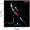 |
Fig. 2. Rest-frame UV image with the F390W filter of HST of the Cosmic Snake galaxy’s isolated counter-image. The red contours correspond to the ALMA CO(4–3) velocity integrated intensity in levels of 4σ, 5σ, 6σ, 7σ, 8σ, and 10σ with an RMS noise of 0.025 Jy beam−1 km s−1. The ALMA beam (0.21″ × 0.18″) is displayed in blue. |
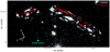 |
Fig. 3. Rest-frame UV image with the F390W filter of HST of the A521. The red contours correspond to the ALMA CO(4–3) velocity integrated intensity in levels of 4σ, 5σ, 6σ, 7σ, 8σ, 10σ, 12σ, and 14σ with an RMS noise of 0.010 Jy beam−1 km s−1. The ALMA beam (0.19″ × 0.16″) is displayed in blue. The green crosses indicate bright foreground sources. |
Properties of the Cosmic Snake and A521.
2.2. HST observations
We used the image of MACS J1206.2−0847 observed in F390W with WFC3/UVIS in the context of the Cluster Lensing And Supernova survey with Hubble (CLASH) as this filter corresponds to rest-frame ultraviolet (UV) wavelengths1. The map we used has a point spread function (PSF) resolution of ∼0.1″ and a pixel scale of 0.03″ (Cava et al. 2018), and the exposure time was ∼4959 s. A full description of the CLASH dataset can be found in Postman et al. (2012).
We took the A521 images observed in F390W with WFC3/UVIS from the HST archive (ID: 15435, PI: Chisholm). The exposure time was 2470 s. The software Multidrizzle (Koekemoer et al. 2007) was used to align and combine in a single image individual calibrated exposures. The final image has a PSF resolution of 0.097″ and a pixel scale of 0.06″ (Messa et al. 2022).
2.3. ALMA observations
The CO(4–3) emission of the Cosmic Snake was detected with ALMA in band 6 at 226.44 GHz, corresponding to a redshift of z = 1.03620. The observations were acquired in Cycle 3 (project 2013.1.01330.S) in the extended C38-5 configuration with a maximum baseline of 1.6 km and 38 antennas of the 12 m array. The total on-source integration time was 52.3 min (Dessauges-Zavadsky et al. 2019). The isolated counter-images of the Cosmic Snake and A521 were observed in band 6 in Cycle 4 (project 2016.1.00643.S) in the C40-6 configuration with a maximum baseline of 3.1 km and 41 antennas of the 12 m array. For the isolated counter-image of the Cosmic Snake, the total on-source time was 51.8 min. For A521, it was 89.0 min. The CO(4–3) line in A521 was detected at 225.66 GHz, which corresponds to a redshift of z = 1.04356 (Dessauges-Zavadsky et al. 2023). The spectral resolution was set to 7.8125 MHz for all three observations.
The data reduction was performed using the standard automated reduction procedure from the pipeline of the Common Astronomy Software Application (CASA) package (McMullin et al. 2007). Briggs weighting was used to image the CO(4–3) emission with a robust factor of 0.5. Using the clean routine in CASA interactively on all channels until convergence, the final synthesised beam size obtained for the Cosmic Snake galaxy was 0.22″ × 0.18″ with a position angle of 85° for the arc, and 0.21″ × 0.18″ with an angle of 49° for the isolated counter-image. For A521 the final synthesised beam size was 0.19″ × 0.16″ at −74°. The adopted pixel scale for the CO(4–3) data cube is 0.04″ for the Cosmic Snake arc and 0.03″ for the Cosmic Snake isolated counter-image and A521. The achieved root mean square (RMS) values are 0.29 mJy beam−1, 0.42 mJy beam−1, and 0.20 mJy beam−1, per 7.8125 MHz channel, for the Cosmic Snake arc, the Cosmic Snake isolated counter-image, and A521, respectively. The CO(4–3) moment-zero maps were obtained using the immoments routine from CASA by integrating the flux over the total velocity range where CO(4–3) emission was detected.
3. Methodology
3.1. Gravitational lens model
The gravitational lens models used for the Cosmic Snake and A521 galaxies are constrained by multiple images found in HST observations. Lenstool (Jullo et al. 2007) was used to compute and optimise the models. The RMS accuracies of the lens models for the positions in the image plane of the Cosmic Snake and A521 galaxies are 0.15″ and 0.08″, respectively. More details on the gravitational lens models used for the Cosmic Snake and A521 can be found in Cava et al. (2018) for the Cosmic Snake, and in Richard et al. (2010) and Messa et al. (2022) for A521.
3.2. Convolution
Since we compared quantities derived from ALMA and HST fluxes in small regions of the galaxies, we ensured that our HST and ALMA maps of a given galaxy were comparable by matching their resolutions. First, we adjusted the pixel scale of the HST and ALMA images, and then we convolved the HST images with the synthesised beam of the ALMA observations, and the ALMA images with the PSF of HST.
3.3. Determination of physical quantities
3.3.1. Molecular gas mass
We used the CO(4–3) line detected with ALMA as the tracer of Mmol. First, we converted the velocity-integrated flux of the CO(4–3) line (SCOΔV) into luminosity ( ) using this equation from Solomon et al. (1997)

with SCOΔV in Jy km s−1, and where νobs is the observed frequency in GHz, and DL the luminosity distance of the source in Mpc. The luminosity is then converted into Mmol (Dessauges-Zavadsky et al. 2019)
where we used the CO luminosity correction factor  , which was extrapolated from r4, 2 and r2, 1 measured in the Cosmic Snake (Dessauges-Zavadsky et al. 2019) and z ∼ 1.5 BzK galaxies (Daddi et al. 2015), respectively. We assumed the Milky Way CO-to-H2 conversion factor αCO = 4.36 M⊙ (K km s−1 pc2)−1 since both in the Cosmic Snake and A521 αCO was found to be close to the Milky Way value from the virialised mass of detected GMCs (Dessauges-Zavadsky et al. 2019, 2023).
The CO(2–1) line was also detected with the Plateau de Bure Interferometer (PdBI) for the Cosmic Snake (Dessauges-Zavadsky et al. 2019), and with the Institut de radioastronomie millimétrique (IRAM) 30 m single dish antenna for A521 (Dessauges-Zavadsky et al. 2023). In both cases, the total molecular gas content traced by the CO(2–1) emission was identical to that traced by CO(4–3). We therefore conclude that using the CO(4–3) line to trace the molecular gas mass is reliable.
3.3.2. Star formation rate
We used the HST rest-frame UV observations with the F390W filter to compute SFR using Eq. (1) of Kennicutt (1998)

where Lν is the UV luminosity. Furthermore, we applied an extinction correction on the SFR, as in Calzetti (2001), as the UV continuum may be significantly affected by extinction

with the obscuration curve for the stellar continuum ke(λ) = 1.17(−2.156 + 1.509/λ − 0.198/λ2 + 0.011/λ3)+1.78 given by Calzetti et al. (2000), where λ is the rest-frame wavelength in μm. The colour excess E(B − V) was computed in Nagy et al. (2022), in radial bins and in the isolated counter-images of the galaxies, by performing spectral energy distribution (SED) fitting on multiple HST bands. The values of E(B − V) obtained from SED fits are in agreement with the value estimated from the Balmer decrement by Messa et al. (2022).
4. Analysis and discussion
4.1. Integrated Kennicutt–Schmidt law
We measured the integrated ΣMmol and ΣSFR on the isolated counter-image to the north-east of the arc for the Cosmic Snake, and on the counter-image to the east for A521. These counter-images show the entire galaxy for both galaxies, unlike the arcs where only a fraction of the galaxy is imaged. To compute ΣMmol and ΣSFR we used the following method. We integrated both the CO(4–3) emission and the UV flux inside the half-light radius measured in the F160W band (Nagy et al. 2022), and then we converted them into the corresponding physical quantities Mmol (using Eqs. (1) and (2)) and SFR (using Eq. (3)), by correcting the SFR for extinction using E(B − V) computed in the same counter-images. To obtain ΣMmol and ΣSFR we then divided by the respective half-light surfaces of the galaxies in the image plane. As the fluxes and the surfaces were both measured in the image plane, there is no need to correct for gravitational lensing if we assume a uniform amplification over the integration area. This is a fair assumption because the magnification varies only by ∼0.3 and ∼0.5 over the counter-images of the Cosmic Snake and A521, respectively.
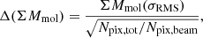
The uncertainty on ΣMmol (Δ(ΣMmol)) was computed following
where ΣMmol(σRMS) is the root mean square noise (σRMS) around the galaxy converted into ΣMmol units, Npix, tot is the total number of pixels inside the integration area, and Npix, beam is the number of pixels in the beam. The uncertainty on ΣSFR (Δ(ΣSFR)) was computed following
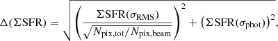
where ΣSFR(σRMS) is the root mean square noise (σRMS) around the galaxy converted into ΣSFR, and ΣSFR(σphot) is the photometric error converted into ΣSFR. We add the magnification uncertainties in quadrature, although they are negligible in comparison to other sources of uncertainties.
We find for the Cosmic Snake ΣSFR = 1.5 ± 0.1 M⊙ yr−1 kpc−2 and ΣMmol = 570 ± 60 M⊙ pc−2. For A521 we have ΣSFR = 1.8 ± 0.1 M⊙ yr−1 kpc−2 and ΣMmol = 430 ± 50 M⊙ pc−2. We show in Fig. 4 the Cosmic Snake and A521 in the (integrated) KS diagram (ΣSFR − ΣMmol), along with a compilations of 25 galaxies from Genzel et al. (2010; z = 1 − 2.5), 73 galaxies from Tacconi et al. (2013; z = 1 − 2.4), and 4 galaxies from Freundlich et al. (2013; z ∼ 1.2). These galaxies are all MS star-forming galaxies (SFGs). We also plot the slope from de los Reyes & Kennicutt (2019) for local spiral galaxies, as well as the slope obtained for stacks of MS SFGs by Wang et al. (2022) at z = 0.4 − 3.6. The Cosmic Snake and A521 are clearly within the distribution of z ≳ 1 galaxies.
 |
Fig. 4. Integrated KS relation of the Cosmic Snake (red) and A521 (purple), along with a compilation of z = 1 − 2.5 galaxies from Genzel et al. (2010; yellow), Tacconi et al. (2013; green), and Freundlich et al. (2013; violet). The blue line is the slope obtained by Wang et al. (2022) for MS SFGs at z = 0.4 − 3.6. The dashed black line is the slope obtained for local galaxies by de los Reyes & Kennicutt (2019). The shaded areas indicate the uncertainties of the respective slopes. |
Furthermore, the compilation of z ≳ 1 galaxies globally satisfies the KS relation with a slope of 1.13 ± 0.09 (Wang et al. 2022), and thus higher than z = 0 galaxies. This steeper slope implies, for a given ΣMmol, a higher ΣSFR in distant galaxies than in the nearby ones. This might indicate that z ≳ 1 galaxies have higher star formation efficiencies. This is indeed the case since the study of the integrated star formation efficiencies (SFE = Mmol/SFR) of MS galaxies shows a mild increase in SFE with redshift (Tacconi et al. 2018; Dessauges-Zavadsky et al. 2020; Wang et al. 2022).
4.2. Resolved Kennicutt–Schmidt law
We studied the rKS law in different bin sizes in the Cosmic Snake and A521. To do so we created six grids paving the reconstructed source plane images of each galaxy, with boxes of 200 pc, 400 pc, 800 pc, 1600 pc, 2800 pc, and 3200 pc for the Cosmic Snake, and 200 pc, 400 pc, 800 pc, 1600 pc, 3200 pc, and 6400 pc for A521. We considered an additional larger bin size in A521 as the galaxy is more extended than the Cosmic Snake, with star formation happening up to a galactocentric radius of 8 kpc and molecular gas detected up to 6 kpc, compared to, respectively, 7 kpc and 1.7 kpc in the Cosmic Snake (Nagy et al. 2022). We then lensed the grids in the corresponding image plane. Due to the differential lensing, the area of some of these boxes is smaller than the matched PSF (HST PSF convolved with ALMA beam) in the image plane, so we discarded those boxes. This is the case for about half of the boxes of 200 pc, and 20% of the boxes of 400 pc. We then measured ΣMmol and ΣSFR inside each of the remaining boxes for both galaxies. In A521, one cluster member is present in front of a small part of the arc (corresponding to the upper green cross in Fig. 3). It has no significant diffuse emission so we simply masked it for our analysis.
To estimate the flux inside a given box from the ALMA maps, we applied the technique developed for the Cosmic Snake galaxy in Dessauges-Zavadsky et al. (2019) in the context of the search of molecular clouds. The method takes into account the three dimensions of the CO(4–3) datacube. To evaluate the detection threshold, the fidelity was computed as
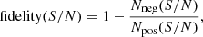
where Npos and Nneg are respectively the number of positive and negative emission detections with a given signal-to-noise ratio (S/N) in the primary beam (Walter et al. 2016; Decarli et al. 2019). The fidelity of 100% was achieved at S/N = 4.4 in individual channel maps in both the Cosmic Snake and A521, and when considering co-spatial emission in two adjacent channels, it was reached at S/N = 4.0 in the Cosmic Snake and at S/N = 3.6 in A521. Therefore, in the ALMA datacube of the Cosmic Snake, we extracted for a given box the emission from each individual channel where the flux inside the box was above a 4.4σ RMS threshold, or above a 4.0σ threshold if the flux inside the same box in an adjacent channel was also above 4.0σ. We did the same for the ALMA maps of A521 with thresholds of 4.4σ and 3.6σ, respectively. Boxes below the ALMA RMS detection threshold were excluded, we did not consider upper limits. The HST flux is always detected where we detect CO. For each box we applied the extinction correction corresponding to the radial bin (computed in Nagy et al. 2022) where the majority of the pixels of the box lies. The uncertainties on Mmol and SFR were computed inside each box following Eqs. (5) and (6), respectively.
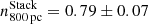
The results for the rKS relation in the Cosmic Snake and A521 are displayed in Figs. 5 and 6, respectively; each panel corresponds to a different bin size. We display with orange squares the ΣMmol values corresponding to the means in six x-axis bins with and equal number of datapoints. By performing a linear regression on all datapoints using the Levenberg–Marquardt algorithm2 and least squares statistic in the Cosmic Snake for scales ≤1600 pc, we obtain slopes of  ,
,  ,
, 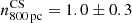 , and
, and 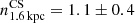 . Uncertainties in the slope measurements increase with spatial scale due to the decrease in the number of datapoints. For the Cosmic Snake, the overall slope of the distribution for the bin sizes ≤1600 pc is similar to the slope reported for local galaxies. For larger scales (> 1600 pc) the number of boxes is too low for a reliable fit. For A521, no overall slope can be inferred at any bin size. The horizontal alignment of the binned means in Fig. 6 can be due to a lack of correlation in the data, as the binned means of a random distribution of points has the same horizontal alignment. We investigate below the differences between the two galaxies and, in particular, in the context of nearby samples from the literature.
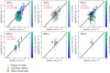 |
Fig. 5. rKS diagram of the Cosmic Snake at different spatial scales. Each panel corresponds to a given bin size in the source plane, as indicated. The contours plotted in the first two panels are kernel density estimates of the data. The five different contours correspond (from inside to outside) to 10%, 30%, 50%, 70%, and 90% iso-proportions of the density. The black line is the rKS slope obtained by Pessa et al. (2021) at the closest spatial scale to ours (n100 pc = 1.06, n500 pc = 1.06, and n1 kpc = 1.03), with the grey shaded area showing the corresponding scatter (σ100 pc = 0.41, σ500 pc = 0.33, and σ1 kpc = 0.27). The datapoints are coloured according to their galactocentric distance, as shown in the colour bars. The orange squares correspond to the ΣSFR means of datapoints within six ΣMmol bins with and equal number of datapoints. Reported in the upper left corner is the scatter (σ) of the datapoints with respect to the fits from Pessa et al. (2021), as well as the slopes (n) obtained from a linear fitting for the bin sizes between 200 pc and 1600 pc. |
In order to determine what is driving the difference in the distribution of datapoints between the two galaxies, we investigated the galactocentric effect, and used a colour-coding depending on the galactocentric distance of each box. For the smaller scales of 200 pc and 400 pc we clearly see a segregation with the galactocentric distance in the Cosmic Snake galaxy. The boxes closer to the centre have much higher ΣSFR and ΣMmol values than those at large galactocentric radii. The Cosmic Snake has steep radial profiles of ΣSFR and ΣMmol (Nagy et al. 2022), so seeing a correlation between the galactocentric distance and the positions of the datapoints in the rKS diagram is not surprising. In A521, no segregation with the galactocentric distance is seen. This is in line with the shallow radial profiles of ΣSFR and ΣMmol in A521, and hence no significant difference in the rKS diagram between regions closer to the centre and regions in the outskirts is seen.
Pessa et al. (2021) measured the rKS in 18 star-forming galaxies from the Physics at High Angular resolution in Nearby GalaxieS (PHANGS3) survey, at scales of 100 pc, 500 pc, and 1 kpc. They reported slopes4 of n100 pc = 1.06 ± 0.01, n500 pc = 1.06 ± 0.02, and n1 kpc = 1.03 ± 0.02, respectively, concluding that no evidence of systematic dependence on spatial scale is shown by the slopes. The slopes of local galaxies match those of the Cosmic Snake within the error bars, although our measurements have much bigger uncertainties due to sparser sampling.
Moreover, in both galaxies, and specifically in A521, we lack dynamical range in ΣSFR and ΣMmol, especially for small values, to consistently constrain the rKS slope in z ∼ 1 galaxies. ΣSFR spans ∼3.5 orders of magnitude in the Cosmic Snake and ∼2.5 in A521, compared to ∼5 in the sample of 18 galaxies from Pessa et al. (2021), and ΣMmol spans ∼2 orders of magnitude in the Cosmic Snake and in A521, compared to ∼3 in Pessa et al. (2021). Higher sensitivity observations could allow us to refine the estimation of the slope in the Cosmic Snake or to estimate the slope in A521. It is important to note, however, that the lack of dynamical range in A521 is not only due to a poor S/N as the Cosmic Snake has a S/N comparable to that of A521, but a much better dynamical range.
We plot the combined rKS of the Cosmic Snake and A521 in Fig. 7 in order to increase the dynamical range of ΣSFR and ΣMmol. The slopes of the stacks (nStack) are 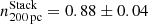 ,
, 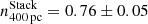 ,
,  , and
, and 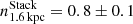 . These slopes are shallower than the slopes of the Cosmic Snake galaxy alone, and also than the slopes obtained by Pessa et al. (2021). The reason is that A521 has a high density of points below the rKS line from Pessa et al. (2021), as illustrated by the contours in Fig. 6. One possible reason that these points have such a low SFR may be that the extinction is underestimated, and specifically where the molecular gas density is high. It may also be due to the SFR tracer we use (rest-frame UV), which traces star-forming regions with ages ∼100 Myr. For a long continuous star formation history (SFH), the estimated SFR by Eq. (3) would be accurate. However, in the case of a more bursty star formation with a constant SFH over a shorter time frame of ∼10 Myr, Eq. (3) underestimates the real SFR.
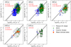 |
Fig. 7. Same as Figs. 5 and 6, but for the combination of the Cosmic Snake and A521. The datapoints are no longer coloured according to galactocentric distance. Instead, the colour indicates the corresponding galaxy: green for A521 and blue for the Cosmic Snake. |
For each set of datapoints at a given bin size, we compute the scatter in dex (σ) as the standard deviation of the datapoints around the rKS power law fits from Pessa et al. (2021) at the closest reported spatial scale (100 pc, 500 pc, or 1 kpc). We use this method instead of computing the scatter around the best-fitting power law, as in Pessa et al. (2021), due to the uncertainty of the fit for the Cosmic Snake, and the meaningless fit if performed for A521. The values are reported in Table 2. Although the number of datapoints per grid binning size and the global shape of their distribution is notably different between the Cosmic Snake and A521, their respective scatters are similar at bin sizes up to 800 pc. The scatter of the two galaxies is also similar to the stack of the two at those scales. At 1600 pc the scatter of the Cosmic Snake decreases significantly, whereas that of A521 stays constant up to 3200 pc, then it decreases as well. The scatter decrease with increasing spatial scale is consistent with the results from Bigiel et al. (2008), Schruba et al. (2010), and Leroy et al. (2013). As a comparison, Pessa et al. (2021) reported scatters for the rKS law of σ100 pc = 0.41, σ500 pc = 0.33, and σ1 kpc = 0.27. They argued that the decrease in scatter at increasing spatial scales is due to the averaging out of small-scale variations.
Scatter (σ) of the rKS at spatial scales of 200 pc, 400 pc, 800 pc, 1.6 kpc, 3.2 kpc, and 6.4 kpc, computed as the standard deviation with respect to the fits from Pessa et al. (2021) at the closest spatial scale.
4.3. Scale dependence of the ΣSFR − ΣMmol spatial correlation
We investigate the scale dependence of the spatial correlation between ΣSFR and ΣMmol in the Cosmic Snake and A521. As in Schruba et al. (2010), we do this by considering τdep = ΣMmol/ΣSFR. The value of τdep is computed for apertures centred on CO and rest-frame UV peaks. The peaks were identified in the arcs of both galaxies, using the CO(4–3) emission from ALMA by Dessauges-Zavadsky et al. (2019) for the Cosmic Snake and by Dessauges-Zavadsky et al. (2023) for A521, and the rest-frame UV emission from HST by Cava et al. (2018) for the Cosmic Snake and Messa et al. (2022) for A521. The CO peaks trace the GMCs, and the rest-frame UV peaks trace the star-forming regions. We then project the locations of the peaks in the source plane, and we centre apertures of different sizes on those positions. We use circular apertures with diameters of 200, 400, 800, 1200, and 1400 pc for the Cosmic Snake, and 400, 800, 1600, 3200, and 6400 pc for A521. These apertures are then lensed into the image plane, and we measure fluxes within each of them. As in Sect. 4.2, we apply a 4.4σ RMS detection threshold to each individual channel of the ALMA datacubes for both the Cosmic Snake and A521, and a 4.0σ detection threshold in the case of co-spatial emission detections in two adjacent channels for the Cosmic Snake and 3.6σ for A521. Again, as the HST rest-frame UV emission is always detected where we also detect CO; we do not apply any detection threshold to the HST maps. We only consider apertures that are larger than the matched PSF in the image plane. We compute an average τdep for each set of apertures of a given size and centred on a given type of peak (CO or UV). The uncertainty of a given average τdep measurement (Δτdep) is computed as
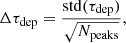
where std(τdep) is the standard deviation of all the τdep used to compute the average, and Npeaks is the number of peaks.
The molecular gas depletion times for apertures of different sizes are given in Fig. 8, showing separately the results for the apertures centred on CO peaks (blue points) and rest-frame UV peaks (red points). The value of τdep varies strongly with the spatial scale (aperture size) and the type of emission targeted (CO or UV). From apertures larger than ∼1 kpc in the Cosmic Snake and ∼6 kpc in A521, the depletion times around CO peaks and those around rest-frame UV peaks converge towards a common value.
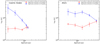 |
Fig. 8. Scale dependence of molecular gas depletion time in Cosmic Snake (left) and A521 (right). The y-axis shows the average of τdep = ΣMmol/ΣSFR for different apertures, and centred on CO peaks (blue points) or on rest-frame UV peaks (red points). The diameters of the apertures are 200, 400, 800, 1200, and 1400 pc for the Cosmic Snake, and 400, 800, 1600, 3200, and 6400 pc for A521. |
The overall behaviour of the molecular gas depletion time curves, commonly known as the tuning fork diagram, resembles that reported in the literature for local galaxies (e.g., Schruba et al. 2010; Kruijssen et al. 2019; Chevance et al. 2020; Kim et al. 2022). However, the uncertainties are much larger for the z ∼ 1 galaxies because of the lack of statistics as the number of detected clumps is about ten times lower than in a typical local galaxy. The τdep convergence seems to happen at slightly larger scales in the Cosmic Snake (≳1 kpc), and much larger scales in A521 (∼6 kpc), than in local galaxies (500 pc − 1 kpc). Some plausible explanations for these differences are given below.
The differences might be due to the difference in tracer; the local studies used Hα as the tracer of star-forming regions, but we used rest-frame UV emission which traces, on average, older star cluster complexes. As a result, the UV clumps that we detect are on average older (∼100 Myr) than the Hα clumps (10 Myr) detected in nearby galaxies. This may imply that the dynamical drift is more significant because UV-bright star-forming regions have moved further away from their parent clouds for a given drift velocity.
The drift of young stars from their parent molecular clouds might be faster in z ∼ 1 galaxies than in local galaxies. This is expected because of the larger gas fraction of high-redshift galaxies, and also because of their higher compactness. Cloud-cloud collisions are enhanced and the gas is more dissipative, while the newly formed stars are collisionless, and decouple faster from the gas. However, as argued in Schruba et al. (2010) and Chevance et al. (2020), the dynamical drift alone, at least in nearby galaxies, is not significant enough to be the cause of such large separations between GMCs and star-forming regions.
Unless the stellar feedback is not strong enough, after 100 Myr the GMC parents of the UV clumps should already be destroyed if their lifetime is comparable to local GMCs (10 − 30 Myr; Kruijssen et al. 2019; Chevance et al. 2020), explaining the lack of correspondence between the CO and UV peaks. Resolved Hα observations are needed to check how significantly the difference in tracers impacts the observed results.
The star-forming regions detected in our high-redshift galaxies might not have been born in the GMCs that we observe, but in other undetected clouds. In other words, there is no correspondence between the GMCs and the star-forming regions that we detect. In the Cosmic Snake and A521, small apertures only contain few a peaks, and the majority are of the kind the aperture is centred on (CO or UV). Apertures of increasing sizes will include more peaks of both kinds, so the ratio of the CO peaks to the UV peaks will converge towards 1. Therefore, the scale dependence of τdep would actually trace the number of CO and UV peaks inside each aperture.
An explanation of the increasing scatter at smaller spatial scales seen in the rKS plots (Figs. 5–7) and discussed in Sect. 4.2 may be found in the divergence at small scales of the molecular gas depletion time curves. At large scales (> 1 kpc in the Cosmic Snake and > 6 kpc in A521), any aperture chosen results in proportional fluxes of molecular gas and SFR tracers, even when focusing specifically at either star-forming regions or GMCs. This means that at these large scales, a randomly selected aperture will likely have a ΣSFR and a ΣMmol that satisfy the rKS relation, and consequently the scatter of the relation for a sample of randomly selected apertures larger than 1 kpc (Cosmic Snake) or 6 kpc (A521) will be low, which is what we observe (Table 2). However, as apertures get smaller, there is much larger scatter because individual star-forming regions are at different stages of time evolution, and thus have different CO-to-UV ratios. Focusing for example on a GMC results in a large τdep because the flux from the tracer of SFR is missed, and τdep is dominated by the numerator ΣMmol (and vice versa). This is the reason for the divergence at small spatial scales seen in Fig. 8. However, when using a random gridding with a small bin size, as in the ΣSFR − ΣMmol plots, the boxes happen to be sometimes between a CO peak and a rest-UV peak, resulting in a datapoint that satisfies the rKS relation, but sometimes they also fall right on a given peak, which yields a datapoint with either a high ΣSFR and a low ΣMmol, or the opposite. This is the cause of the large scatter seen at small scales in the rKS diagrams. As a result, the majority of the datapoints do not satisfy the rKS law at small scales, but the entire cloud of datapoints is centred on it, and even the slope is close to the value obtained for scales > 1 kpc (in the case of the Cosmic Snake). If the rKS law were valid at small scales, any randomly selected aperture would fall on the slope of the relation, within the scatter observed for the largest scales.
5. Conclusions
We analysed the KS law in the Cosmic Snake and A521, two strongly lensed galaxies at z ∼ 1, at galactic integrated scales down to sub-kiloparsec scales. We used the rest-frame UV emission from HST to trace SFR and the CO(4–3) emission line detected with ALMA to trace Mmol. In addition to several multiple images with magnifications of μ > 20 that are significantly stretched and where only a fraction of the galaxy is visible, the two galaxies show an isolated counter-image with overall uniform magnifications of 4.3 and 3 for the Cosmic Snake and A521, respectively. In these counter-images, the entirety of the galaxies is visible, and thus we used them to compute integrated values of SFR and Mmol. We found ΣSFR = 1.5 ± 0.1 M⊙ yr−1 kpc−2 and ΣMmol = 570 ± 60 M⊙ pc−2 in the Cosmic Snake, and ΣSFR = 1.8 ± 0.1 M⊙ yr−1 kpc−2 and ΣMmol = 430 ± 50 M⊙ pc−2 in A521. The two galaxies satisfy the integrated KS relation derived at z = 1 − 2.5 (Genzel et al. 2010; Tacconi et al. 2013; Freundlich et al. 2013; Wang et al. 2022).
To study the rKS law by taking advantage of the strong gravitational lensing in the Cosmic Snake and A521, we defined six different grids in the source plane of each galaxy. We then lensed those grids in the image plane, and computed ΣMmol and ΣSFR inside each box. The grids that we used had sizes of 200 pc, 400 pc, 800 pc, 1600 pc, 2800 pc, and 3200 pc for the Cosmic Snake, and 200 pc, 400 pc, 800 pc, 1600 pc, 3200 pc, and 6400 pc for A521.
We derived the following results from the analysis of the rKS law in the Cosmic Snake and A521:
-
We were able to perform a linear regression on the measurements in the Cosmic Snake for scales ≤1600 pc, obtaining slopes of
 ,
,  ,
,  , and
, and  . These slopes are similar to those typically found in local galaxies. For A521 no overall slope could be inferred at any scale. We measured slopes for the combined rKS of the Cosmic Snake and A521 of
  ,
,  ,
,  , and
, and  .
. -
To consistently constrain the rKS slopes in the analysed z ∼ 1 galaxies, we lack dynamical range in both ΣMmol and ΣSFR. In the study of 18 PHANGS galaxies from Pessa et al. (2021), the two quantities span at least one more order of magnitude than our study.
-
We see a clear spatial segregation in the distribution of the datapoints in the rKS diagram of the Cosmic Snake. Points close to the galactic centre tend to have higher ΣMmol and ΣSFR, whereas measurements in the outskirts show lower values. No such segregation is observed in A521. These observations match the results from Nagy et al. (2022) showing that the Cosmic Snake has much steeper radial profiles than A521, in ΣMmol and ΣSFR in particular.
-
The scatter of the datapoints in the Cosmic Snake and A521 is very similar at small scales up to 800 pc. The scatter of the galaxies decreases at higher scales of 1600 pc for the Cosmic Snake and 6400 pc for A521. The decrease in scatter with increasing bin sizes is similar to what is observed in z = 0 galaxies, and is due to the averaging out of small-scale variations.
We measured the average τdep inside apertures of different diameters centred on either rest-frame UV or CO(4–3) emission peaks in the Cosmic Snake and A521. In both galaxies we observe the same overall behaviour as in local galaxies; that is, the τdep values measured using small apertures are clearly different whether the apertures are centred on rest-frame UV peaks or on CO(4–3) peaks, and they converge towards a common value at large enough spatial scales. In nearby galaxies, the convergence typically happens in apertures of diameters of 500 pc − 1 kpc. In the Cosmic Snake the τdep measurements converge at higher but comparable apertures of size ≳1 kpc, whereas in A521 it happens in much larger apertures of ∼6 kpc.
We conclude that the increasing scatter in the rKS diagrams in small bin sizes is partly explained by the divergence observed between τdep measured when focusing on rest-frame UV peaks and CO(4–3) peaks at small scales. By taking values of ΣSFR and ΣMmol from randomly selected boxes of small sizes, the corresponding datapoint may satisfy the rKS law, but may also be significantly off if the aperture happens to capture only one kind of peak. In boxes larger than the size for which the τdep values converge, any datapoint will tend to fall on the rKS, and hence the smaller scatter. In the Cosmic Snake and A521, the scales at which τdep converges are the scales at which the scatter of those galaxies in the rKS diagram decreases.
The data from CLASH are available at https://archive.stsci.edu/prepds/clash/
The slopes from Pessa et al. (2021) were computed by binning the x-axis and averaging the y-axis values inside each ΣSFR bin, whereas our slopes were computed by taking into account every measurement.
Acknowledgments
This work was supported by the Swiss National Science Foundation. Based on observations made with the NASA/ESA Hubble Space Telescope, and obtained from the Data Archive at the Space Telescope Science Institute, which is operated by the Association of Universities for Research in Astronomy, Inc., under NASA contract NAS 5-26555. These observations are associated with program #15435. This paper makes use of the following ALMA data: ADS/JAO.ALMA#2013.1.01330.S, and ADS/JAO.ALMA#2016.1.00643.S. ALMA is a partnership of ESO (representing its member states), NSF (USA) and NINS (Japan), together with NRC (Canada), MOST and ASIAA (Taiwan), and KASI (Republic of Korea), in cooperation with the Republic of Chile. The Joint ALMA Observatory is operated by ESO, AUI/NRAO and NAOJ. M.M. acknowledges the support of the Swedish Research Council, Vetenskapsrådet (internationell postdok grant 2019-00502). J.S. acknowledges support by the Natural Sciences and Engineering Research Council of Canada (NSERC) through a Canadian Institute for Theoretical Astrophysics (CITA) National Fellowship.
References
- Bayliss, M. B., Rigby, J. R., Sharon, K., Gladders, M. D., & Wuyts, E. 2014, Proc. Int. Astron. Union, 10, 251 [Google Scholar]
- Bigiel, F., Leroy, A., Walter, F., et al. 2008, AJ, 136, 2846 [NASA ADS] [CrossRef] [Google Scholar]
- Calzetti, D. 2001, PASP, 113, 1449 [Google Scholar]
- Calzetti, D., Armus, L., Bohlin, R. C., et al. 2000, ApJ, 533, 682 [NASA ADS] [CrossRef] [Google Scholar]
- Cava, A., Schaerer, D., Richard, J., et al. 2018, Nat. Astron., 2, 76 [Google Scholar]
- Chevance, M., Kruijssen, J. M. D., Hygate, A. P. S., et al. 2020, MNRAS, 493, 2872 [NASA ADS] [CrossRef] [Google Scholar]
- Claeyssens, A., Adamo, A., Richard, J., et al. 2023, MNRAS, 520, 2180 [NASA ADS] [CrossRef] [Google Scholar]
- Daddi, E., Dannerbauer, H., Liu, D., et al. 2015, A&A, 577, A46 [NASA ADS] [CrossRef] [EDP Sciences] [Google Scholar]
- Decarli, R., Walter, F., Gónzalez-López, J., et al. 2019, ApJ, 882, 138 [Google Scholar]
- de los Reyes, M. A. C., & Kennicutt, R. C. 2019, ApJ, 872, 16 [NASA ADS] [CrossRef] [Google Scholar]
- Dessauges-Zavadsky, M., Richard, J., Combes, F., et al. 2019, Nat. Astron., 3, 1115 [NASA ADS] [CrossRef] [Google Scholar]
- Dessauges-Zavadsky, M., Ginolfi, M., Pozzi, F., et al. 2020, A&A, 643, A5 [NASA ADS] [CrossRef] [EDP Sciences] [Google Scholar]
- Dessauges-Zavadsky, M., Richard, J., Combes, F., et al. 2023, MNRAS, 519, 6222 [NASA ADS] [CrossRef] [Google Scholar]
- Feldmann, R., Gnedin, N. Y., & Kravtsov, A. V. 2011, ApJ, 732, 115 [NASA ADS] [CrossRef] [Google Scholar]
- Freundlich, J., Combes, F., Tacconi, L. J., et al. 2013, A&A, 553, A130 [NASA ADS] [CrossRef] [EDP Sciences] [Google Scholar]
- Genzel, R., Tacconi, L. J., Gracia-Carpio, J., et al. 2010, MNRAS, 407, 2091 [NASA ADS] [CrossRef] [Google Scholar]
- Girard, M., Dessauges-Zavadsky, M., Combes, F., et al. 2019, A&A, 631, A91 [NASA ADS] [CrossRef] [EDP Sciences] [Google Scholar]
- Jones, T. A., Swinbank, A. M., Ellis, R. S., Richard, J., & Stark, D. P. 2010, MNRAS, 404, 1247 [NASA ADS] [Google Scholar]
- Jullo, E., Kneib, J.-P., Limousin, M., et al. 2007, New J. Phys., 9, 447 [Google Scholar]
- Kennicutt, R. C. 1998, ARA&A, 36, 189 [NASA ADS] [CrossRef] [Google Scholar]
- Kim, J., Chevance, M., Kruijssen, J. M. D., et al. 2022, MNRAS, 516, 3006 [NASA ADS] [CrossRef] [Google Scholar]
- Koekemoer, A. M., Aussel, H., Calzetti, D., et al. 2007, ApJS, 172, 196 [Google Scholar]
- Kruijssen, J. M. D., Schruba, A., Hygate, A. P. S., et al. 2018, MNRAS, 479, 1866 [NASA ADS] [CrossRef] [Google Scholar]
- Kruijssen, J. M. D., Schruba, A., Chevance, M., et al. 2019, Nature, 569, 519 [NASA ADS] [CrossRef] [Google Scholar]
- Leroy, A. K., Walter, F., Sandstrom, K., et al. 2013, ApJ, 146, 19 [CrossRef] [Google Scholar]
- Livermore, R. C., Jones, T. A., Richard, J., et al. 2015, MNRAS, 450, 1812 [Google Scholar]
- McMullin, J. P., Waters, B., Schiebel, D., Young, W., & Golap, K. 2007 in Astronomical Data Analysis Software and Systems XVI, eds. R. A. Shaw, F. Hill, D. J. Bell, ASP Conf. Ser., 376,127 [NASA ADS] [Google Scholar]
- Messa, M., Dessauges-Zavadsky, M., Richard, J., et al. 2022, MNRAS, 516, 2420 [Google Scholar]
- Nagy, D., Dessauges-Zavadsky, M., Richard, J., et al. 2022, A&A, 657, A25 [NASA ADS] [CrossRef] [EDP Sciences] [Google Scholar]
- Patrício, V., Richard, J., Carton, D., et al. 2018, MNRAS, 477, 18 [Google Scholar]
- Patrício, V., Richard, J., Carton, D., et al. 2019, MNRAS, 489, 224 [Google Scholar]
- Pessa, I., Schinnerer, E., Belfiore, F., et al. 2021, A&A, 650, A134 [NASA ADS] [CrossRef] [EDP Sciences] [Google Scholar]
- Postman, M., Coe, D., Benítez, N., et al. 2012, ApJS, 199, 25 [Google Scholar]
- Richard, J., Smith, G. P., Kneib, J.-P., et al. 2010, MNRAS, 404, 325 [NASA ADS] [Google Scholar]
- Salpeter, E. E. 1955, ApJ, 121, 161 [Google Scholar]
- Schmidt, M. 1959, ApJ, 129, 243 [NASA ADS] [CrossRef] [Google Scholar]
- Schmidt, M. 1963, ApJ, 137, 758 [Google Scholar]
- Schruba, A., Leroy, A. K., Walter, F., Sandstrom, K., & Rosolowsky, E. 2010, ApJ, 722, 1699 [NASA ADS] [CrossRef] [Google Scholar]
- Solomon, P. M., Downes, D., Radford, S. J. E., & Barrett, J. W. 1997, ApJ, 478, 144 [NASA ADS] [CrossRef] [Google Scholar]
- Sun, J., Leroy, A. K., Ostriker, E. C., et al. 2023, ApJ, 945, L19 [NASA ADS] [CrossRef] [Google Scholar]
- Tacconi, L. J., Neri, R., Genzel, R., et al. 2013, ApJ, 768, 74 [NASA ADS] [CrossRef] [Google Scholar]
- Tacconi, L. J., Genzel, R., Saintonge, A., et al. 2018, ApJ, 853, 179 [Google Scholar]
- Walter, F., Decarli, R., Aravena, M., et al. 2016, ApJ, 833, 67 [Google Scholar]
- Wang, T.-M., Magnelli, B., Schinnerer, E., et al. 2022, A&A, 660, A142 [NASA ADS] [CrossRef] [EDP Sciences] [Google Scholar]
All Tables
Scatter (σ) of the rKS at spatial scales of 200 pc, 400 pc, 800 pc, 1.6 kpc, 3.2 kpc, and 6.4 kpc, computed as the standard deviation with respect to the fits from Pessa et al. (2021) at the closest spatial scale.
All Figures
|
Fig. 1. Rest-frame UV image with the F390W filter of HST of the Cosmic Snake galaxy’s arc. The red contours correspond to the ALMA CO(4–3) velocity integrated intensity in levels of 4σ, 5σ, 6σ, 7σ, 8σ, 10σ, and 12σ with an RMS noise of 0.020 Jy beam−1 km s−1. The ALMA beam (0.22″ × 0.18″) is displayed in blue. The green crosses indicate bright foreground sources. |
| In the text | |
|
Fig. 2. Rest-frame UV image with the F390W filter of HST of the Cosmic Snake galaxy’s isolated counter-image. The red contours correspond to the ALMA CO(4–3) velocity integrated intensity in levels of 4σ, 5σ, 6σ, 7σ, 8σ, and 10σ with an RMS noise of 0.025 Jy beam−1 km s−1. The ALMA beam (0.21″ × 0.18″) is displayed in blue. |
| In the text | |
|
Fig. 3. Rest-frame UV image with the F390W filter of HST of the A521. The red contours correspond to the ALMA CO(4–3) velocity integrated intensity in levels of 4σ, 5σ, 6σ, 7σ, 8σ, 10σ, 12σ, and 14σ with an RMS noise of 0.010 Jy beam−1 km s−1. The ALMA beam (0.19″ × 0.16″) is displayed in blue. The green crosses indicate bright foreground sources. |
| In the text | |
|
Fig. 4. Integrated KS relation of the Cosmic Snake (red) and A521 (purple), along with a compilation of z = 1 − 2.5 galaxies from Genzel et al. (2010; yellow), Tacconi et al. (2013; green), and Freundlich et al. (2013; violet). The blue line is the slope obtained by Wang et al. (2022) for MS SFGs at z = 0.4 − 3.6. The dashed black line is the slope obtained for local galaxies by de los Reyes & Kennicutt (2019). The shaded areas indicate the uncertainties of the respective slopes. |
| In the text | |
|
Fig. 5. rKS diagram of the Cosmic Snake at different spatial scales. Each panel corresponds to a given bin size in the source plane, as indicated. The contours plotted in the first two panels are kernel density estimates of the data. The five different contours correspond (from inside to outside) to 10%, 30%, 50%, 70%, and 90% iso-proportions of the density. The black line is the rKS slope obtained by Pessa et al. (2021) at the closest spatial scale to ours (n100 pc = 1.06, n500 pc = 1.06, and n1 kpc = 1.03), with the grey shaded area showing the corresponding scatter (σ100 pc = 0.41, σ500 pc = 0.33, and σ1 kpc = 0.27). The datapoints are coloured according to their galactocentric distance, as shown in the colour bars. The orange squares correspond to the ΣSFR means of datapoints within six ΣMmol bins with and equal number of datapoints. Reported in the upper left corner is the scatter (σ) of the datapoints with respect to the fits from Pessa et al. (2021), as well as the slopes (n) obtained from a linear fitting for the bin sizes between 200 pc and 1600 pc. |
| In the text | |
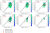 |
Fig. 6. Same as Fig. 5, but for A521. |
| In the text | |
|
Fig. 7. Same as Figs. 5 and 6, but for the combination of the Cosmic Snake and A521. The datapoints are no longer coloured according to galactocentric distance. Instead, the colour indicates the corresponding galaxy: green for A521 and blue for the Cosmic Snake. |
| In the text | |
|
Fig. 8. Scale dependence of molecular gas depletion time in Cosmic Snake (left) and A521 (right). The y-axis shows the average of τdep = ΣMmol/ΣSFR for different apertures, and centred on CO peaks (blue points) or on rest-frame UV peaks (red points). The diameters of the apertures are 200, 400, 800, 1200, and 1400 pc for the Cosmic Snake, and 400, 800, 1600, 3200, and 6400 pc for A521. |
| In the text | |
Current usage metrics show cumulative count of Article Views (full-text article views including HTML views, PDF and ePub downloads, according to the available data) and Abstracts Views on Vision4Press platform.
Data correspond to usage on the plateform after 2015. The current usage metrics is available 48-96 hours after online publication and is updated daily on week days.
Initial download of the metrics may take a while.