| Issue |
A&A
Volume 627, July 2019
|
|
|---|---|---|
| Article Number | A117 | |
| Number of page(s) | 17 | |
| Section | Stellar atmospheres | |
| DOI | https://doi.org/10.1051/0004-6361/201935306 | |
| Published online | 10 July 2019 | |
Chemical (in)homogeneity and atomic diffusion in the open cluster M 67★,★★
1
Lund Observatory, Department of Astronomy and Theoretical physics, Lund University, Box 43, 22100 Lund, Sweden
e-mail: This email address is being protected from spambots. You need JavaScript enabled to view it.
2
Research School of Astronomy and Astrophysics, Australian National University,
Canberra, ACT 2611, Australia
3
ARC Centre of Excellence for All Sky Astrophysics in 3 Dimensions (ASTRO 3D), Canberra, Australia
4
Harvard-Smithsonian Center for Astrophysics,
Cambridge,
MA 02138, USA
5
Departamento de Astronomia do IAG/USP, Universidade de Sao Paulo,
Rua do Matao 1226,
Sao Paulo 05508-900, SP, Brazil
6
Tacoma Community College,
Washington, USA
Received:
19
February
2019
Accepted:
6
June
2019
Abstract
Context. The benchmark open cluster M 67 is known to have solar metallicity and an age similar to that of the Sun. It thus provides us with a great opportunity to study the properties of solar twins, as well as the evolution of Sun-like stars.
Aims. Previous spectroscopic studies of M 67 reported possible subtle changes in stellar surface abundances throughout the stellar evolutionary phase, namely the effect of atomic diffusion. In this study we attempt to confirm and quantify more precisely the effect of atomic diffusion, and to explore the level of chemical (in)homogeneity in M 67.
Methods. We presented a strictly line-by-line differential chemical abundance analysis of two groups of stars in M 67: three turn-off stars and three subgiants. Stellar atmospheric parameters and elemental abundances were obtained with very high precision using the Keck/HIRES spectra.
Results. The subgiants in our sample show negligible abundance variations (≤0.02 dex), which implies that M 67 was born chemically homogeneous. We note that there is a significant abundance difference (~0.1–0.2 dex) between subgiants and turn-off stars, which can be interpreted as the signature of atomic diffusion. Qualitatively stellar models with diffusion agree with the observed abundance results. Some turn-off stars do not follow the general pattern, which suggests that in some cases diffusion can be inhibited, or they might have undergone some sort of mixing event related to planets.
Conclusions. Our results pose additional challenges for chemical tagging when using turn-off stars. In particular, the effects of atomic diffusion, which could be as large as 0.1–0.2 dex, must be taken into account in order for chemical tagging to be successfully applied.
Key words: stars: abundances / stars: atmospheres / stars: evolution / open clusters and associations: individual: NGC 2682
Table A.1 is only available at the CDS via anonymous ftp to cdsarc.u-strasbg.fr (130.79.128.5) or via http://cdsarc.u-strasbg.fr/viz-bin/qcat?J/A+A/627/A117
The data presented here were obtained at the W.M. Keck Observatory, which is operated as a scientific partnership among the California Institute of Technology, the University of California, and the National Aeronautics and Space Administration. The Observatory was made possible by the generous financial support of the W.M. Keck Foundation.
© ESO 2019
1 Introduction
Stars form in clustered environments. It is often assumed that the gas in proto-clusters is well-mixed, which means that the stars that form from that gas should all have the same chemical composition (e.g. De Silva et al. 2006, 2007; Feng & Krumholz 2014). Open clusters dissolve on timescales that are short compared to Galactic timescales, thus the clusters build up the field stellar population when they dissolve. The assumption of chemical homogeneity in the clustered environments where stars form inspired the concept of chemical tagging. The idea of chemical tagging is that by obtaining precise elemental abundances we will be able to identify the star-forming events that first provided the stars and/or identify how many such star-forming regions have contributed to the stellar field population and help us to recreate, for example, the star formation history of the stellar disc (Freeman & Bland-Hawthorn 2002). This is a very exciting prospect that merits detailed scrutiny. In a series of investigations we study different cases that will help us to quantify the power of chemical tagging.
The first aspect to investigate is whether open clusters, those that have not yet dissolved, actually are chemically homogenous. We have found that in fact not all clusters are chemically homogenous. We also find that the level of chemical inhomogeneity can be different for light and heavy elements. This was found for the first time in the open cluster Hyades by Liu et al. (2016a), with a strictly line-by-line differential analysis and extremely high precision (σ < 0.02 dex). It thus appears that if a precision of less than 0.03 dex is needed to chemically tag star-forming regions, then current surveys might find the task challenging.
Another aspect that must be accounted for is the fact that many stars have planets and it is now understood that it is possible that planet formation might affect the chemical composition of the host star (see e.g. Meléndez et al. 2009; Ramírez et al. 2010; Liu et al. 2016b). This could lead to changes in the surface abundance of some elements. Spina et al. (2018) conducted a high-precision spectroscopic study of five members of the open cluster Pleiades and reported variations in the elemental abundances. They attributed the observed chemical inhomogeneity to the process of forming planets since the abundance differences correlate with condensation temperature of the elements analysed. One hypothesis is that the refractory materials (elements with high condensation temperature) in the proto-stellar nebula were locked up in the terrestrial planets. The remaining dust-cleansed gas was then accreted on to the host star. Therefore the stars hosting terrestrial planets might be depleted in refractories. Also, planets could be accreted onto their host stars, causing an increase in the abundances of refractory elements.
A third important fact is that even if all stars in an open cluster initially have the same chemical composition, physical processes will change the elemental abundances in their surface layers. One important and little studied process that changes the elemental abundances in the surface layers is atomic diffusion. Atomic diffusion is a combination of the effect of gravitational settling, forcing different elements to sink to below the convection zone of the star, and radiative acceleration playing against it (Michaud et al. 1984, 2015). Atomic diffusion is expected to alter the elemental abundances in the upper layers of a star depending on the star’s evolutionary stage. The elemental abundances in the surface layers should decrease when the star evolves along the main sequence until they reach the turn-off point. After that the convection zone in the star will deepen and thus will start to restore the original chemical composition in the atmosphere during the subgiant and red giant phases. Therefore we need to use stellar evolutionary models to infer the original chemical abundances of stars from what we observe (Dotter et al. 2017), in order to use the stars for chemical tagging exercises.
Several studies have reported on variations of elemental abundances for different evolutionary stages in metal-poor globular clusters like NGC 6397 (see e.g. Korn et al. 2007; Lind et al. 2008; Nordlander et al. 2012). Similar phenomena were detected in NGC 6752 at higher metallicities (Gruyters et al. 2013), although with smaller amplitude of the variations in the elemental abundances.However, it is more challenging to test the effect of atomic diffusion in the open clusters since the expected signature is very small particularly for solar mass, solar metallicity, and solar age objects (see e.g. Dotter et al. 2017).
M 67 is an old benchmark open cluster that offers great opportunities to study the effect of stellar evolution of Sun-like stars. The metallicity for main sequence stars in M 67 have been measured to be similar to that of the Sun (Pasquini et al. 2008; Önehag et al. 2011, 2014; Liu et al. 2016c). The age of M 67 is about 4 Gyr (Yadav et al. 2008; Sarajedini et al. 2009), also comparable with that of the Sun. This makes M 67 an ideal target to probe and test the effect of atomic diffusion and the related stellar evolution models. M 67 has been studied by several high-resolution spectroscopic studies in recent years. Önehag et al. (2011) presented the first high-resolution analysis of a solar twin in M 67 and found that it has a similar chemical composition to that of the Sun. Önehag et al. (2014) observed the reduction in surface abundances of heavy elements of the dwarfs and turn-off point stars relative to the subgiants and they suspected this could be due to the processes of diffusion. Liu et al. (2016c) studied two solar twins in M 67 and confirmed that their chemical abundances are identical to that of the Sun for the elements with atomic number (Z) ≤ 30, while one of the solar twins is enriched for the neutron-capture elements, possibly due to the contribution of its binary companion. Souto et al. (2018) reported the detection of a possible effect of atomic diffusion by studying a total of eight stars in different evolutionaryphases, using the spectra from the Apache Point Observatory Galactic Evolution Experiment (APOGEE) with resolution of ~20 000. Three later studies also found a similar effect using the spectra from the GALactic Archaeology with HERMES (GALAH) survey (Gao et al. 2018), Gaia-ESO spectra (Bertelli Motta et al. 2018), and APOGEE spectra of additional stars (Souto et al. 2019). In these studies, the abundance differences between the turn-off and subgiant stars were 0.05–0.07 dex, comparable to the typical measurement uncertainties. A more compelling demonstration of atomic diffusion in this cluster would be provided if the abundance errors were a factor of 2–3 smaller than the atomic diffusion signature.
In this paper, we presented a strictly line-by-line differential elemental abundance analysis of three turn-off stars and three subgiant stars in the old open cluster M 67. For the analysis we obtained high-resolution, very high signal-to-noise ratio (S/N) spectra. We used these spectra to examine the possible effect of atomic diffusion in this old open cluster.
2 Observations and data reduction
We carefully selected our targets depending on their position in the colour–magnitude diagram (see Fig. 1). In particular we selected stars in two groups: turn-off stars and subgiant stars. We note that our programme stars, taken from Yadav et al. (2008), are all members of M 67 at a high level of probability based on their proper motions. According to the Gaia Data Release 2 (Gaia Collaboration 2018), our sample stars also have very similar parallaxes, around 1.0848 mas, further confirming their membership. The basic data for our sample stars are listed in Table 1.
For this project, we observed three turn-off stars (Y1388, Y535, and Y2235) and three subgiant stars (Y1844, Y519, and Y923). We obtained the high-resolution (R = λ∕Δλ = 50 000), high S/N spectra with the 0.86″ slit, kv408 filter of the High Resolution Echelle Spectrometer (HIRES, Vogt et al. 1994) on the 10 m Keck I telescope during the nights of February 1, April 8, and April 9, 2017. The spectral wavelength coverage is nearly complete from 400 to 840 nm.
The Keck-MAKEE pipeline was used for standard echelle spectra reduction including bias subtraction, flat fielding, scattered-light subtraction, spectra extraction and wavelength calibration. We normalized, barycentric velocity corrected, and co-added the spectra using packages within IRAF1. The spectrum of each star has been radial velocity (RV) calibrated to the rest wavelength, using the rv package of IRAF. The individual frames of each star were combined into a single spectrum with S∕N ≈ 250–300 per pixel in most wavelength regions. We note that one of our programme stars (Y535) shows RV variation when compared to the other stars, which indicates that this star might have a wide binary companion. We note that no double-line features could be identified in the spectrum of Y535. Portions of the reduced spectra for the subgiant and turn-off stars are shown in Fig. 2.
We included a solar spectrum by observing the asteroid Hebe (S∕N ≈ 450 per pixel); we also included the spectrum of a main sequence solar twin in M 67 (Y1194, S∕N ≈ 270 per pixel) in this study. Thesetwo spectra2 share the same instrumental configuration as the spectra of our programme stars, and were reduced using the same method.
The spectral line list of 22 elements (C, O, Na, Mg, Al, Si, S, Ca, Sc, Ti, V, Cr, Mn, Fe, Co, Ni, Cu, Zn, Sr, Y, Ba, and Ce) used in our analysis was adopted mainly from Scott et al. (2015a,b) and Grevesse et al. (2015), and complemented with additional unblended lines from Bensby et al. (2005) and Meléndez et al. (2014). Equivalent widths were measured manually using the splot task in IRAF. We note that each spectral line was measured consecutively for all the programme stars by setting a consistent continuum, resulting in precise measurements in a differential sense. Strong lines with EW ≥ 120 mÅ were excluded from the analysis to limit the effects of saturation with the exception of a few Mg I, Mn I, and Ba I lines. The atomic line data and the measured equivalent widths that we adopted for our analysis are listed in Table A1.
Information of our programme stars.
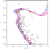 |
Fig. 1 Our programme stars in the colour magnitude diagram, selected from Yadav et al. (2008), all with a high probability of membership. The red symbols correspond to our targets: solar twin Y1194 (red circle), turn-off stars (red rectangles), subgiant stars (red triangles). The blue, magenta, and red solid lines correspond to the isochrones for an age of 4 Gyr, |

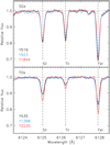 |
Fig. 2 Top panel: portion of the reduced spectra for the subgiant stars in our sample; Y519, Y923, and Y1844 are plotted in black, blue, and red, respectively. A few atomic lines (Si I, Ti I, Fe I) used in our analysis in this region are marked by the dashed lines. Bottom panel: similar to the top panel, but for the turn-off stars in our sample; Y535, Y1388, and Y2235 are plotted in black, blue, and red, respectively. |
3 Analysis and results
In this section we present the process of data analysis and our results, including stellar atmospheric parameters and elemental abundances.
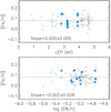 |
Fig. 3 Top panel: [Fe/H] of Y923 derived on a line-by-line basis with respect to the Sun as a function of LEP; open circles and blue filled circles represent Fe I and Fe II lines, respectively. The black dotted line shows the location of mean [Fe/H], the green dashed line represents the linear least-squares fit to the data. Bottom panel: same as the top panel, but as a function of reduced equivalent width. |
3.1 Stellar atmospheric parameters
We conducted a 1D, local thermodynamic equilibrium (LTE) elemental abundance analysis using MOOG (version 2014, Sneden 1973; Sobeck et al. 2011) with the Kurucz model atmospheres (ODFNEW grid, Castelli & Kurucz 2003). Stellar atmospheric parameters (i.e. effective temperature Teff, surface gravity log g, microturbulent velocity ξt, and metallicity [Fe/H]) were obtained by forcing differential excitation and ionization balance of Fe I and Fe II lines on a strictly line-by-line basis relative to the Sun (reflected light from the Hebe asteroid). The following parameters for the Sun were adopted: Teff = 5772 K, log g = 4.44 (cm s−2), ξt = 1.00 km s−1, and [Fe/H] = 0.00. The stellar parameters of our programme stars were derived individually using an automatic grid searching technique described in Liu et al. (2014). Briefly, the best combination of stellar atmospheric parameters, which minimized the slopes in [Fe I/H] versus lower excitation potential (LEP) and reduced equivalent width (log (EW/λ) as well as the difference between [Fe I/H] and [Fe II/H], was determined from a successively refined grid of stellar atmospheric models. The final solution was achieved when the grid step-size decreased to ΔTeff = 1 K, Δ log g = 0.01 (cm s−2), and Δξt = 0.01 km s−1. We also require the derived average [Fe/H] to be consistent with the adopted model atmospheric value. Lines whose elemental abundances departed from the average by more than 3 σ were clipped. Figure 3 shows an example of obtaining the stellar atmospheric parameters of the subgiant star Y923 relative to the Sun. The adopted stellar parameters satisfy the excitation and ionization balance in a differential sense.
The final adopted stellar atmospheric parameters of our programme stars, and the data for the solar twin Y1194 and the Sun and their parameters as a reference point, are listed in Table 2. The adopted uncertainties in the stellar parameters were calculated using the method described by Epstein et al. (2010) and Bensby et al. (2014), which accounts for the co-variances between changes in the stellar parameters and the differential iron abundances. High precision was achieved thanks to the high-quality spectra and the strictly line-by-line differential method, which greatly reduces the systematic errors from atomic line data and from shortcomings in the 1D LTE modelling of the stellar atmospheres and spectral line formation (see e.g. Asplund et al. 2009). In this study, we were able to reproduce the results for the solar twin Y1194 as we did in our previous study (Liu et al. 2016c). In addition, we repeated the whole analysis by choosing a typical subgiant star (Y923) and a typical turn-off star (Y1388) as a reference. The results are essentially the same, albeit with slightly different uncertainties, and do not change our final results and conclusion. Since the parameters of the Sun are closer to both turn-off and subgiant stars, leading to results with slightly smaller uncertainties, we chose the Sun as the reference star in the following analyses. We note that the overall metallicities of the subgiant stars are higher than that of the turn-off stars by more than 0.1 dex. We also note that the turn-off star Y2235 has a highermetallicity than the other two other turn-off stars. A detailed discussion of this outlier is presented in Sect. 4.2.
We compared the stellar parameters derived from this study to several previous spectroscopic studies for the stars in common. Our turn-offstar Y1388 has been studied in Gao et al. (2018) and our subgiant star Y1844 in the two studies (Gao et al. 2018; Souto et al. 2018). For both stars, our results agree well with the previous studies in terms of Teff and log g with consideration of the estimated errors. The metallicity ([Fe/H]) for Y1388 in this study is higher than that from Gao et al. (2018) by ≈ 0.07 dex, while [Fe/H] for Y1844 in this studyis higher by ≈0.08 dex and 0.05 dex than that from Gao et al. (2018) and Souto et al. (2018), respectively. The differences in [Fe/H] are most likely due to a zero-point offset, which has little impact on the conclusion. As mentioned in Sect. 1, we have achieved our goal of obtaining a precision that is two or three times better than the previous studies mainly because our spectra have higher resolution (especially when compared to APOGEE spectra), as well as higher S∕N (250– 300 in this study; 50–150 in previous studies).
3.2 Elemental abundances
Having established the stellar atmospheric parameters of our programme stars, we then derived abundances for 21 elements in addition to Fe (C, O, Na, Mg, Al, Si, S, Ca, Sc, Ti, V, Cr, Mn, Co, Ni, Cu, Zn, Sr, Y, Ba, and Ce) based on the spectral lines and measured equivalent widths listed in Table A1. We derived line-by-line differential elemental abundances ([X/H]) of our programme stars relative to the Sun. We note that we considered one element with different ionization stages as two species in our analysis, rather than combining their elemental abundances together. We took hyperfine structure (HFS) into account for six elements (Sc, V, Mn, Co, Cu, and Ba) and calculated corrections strictly line by line. The HFS data were taken from Kurucz & Bell (1995) for Sc, V, Co, Cu, and Ba. For Mn, the HFS corrections were applied using the data from Prochaska et al. (2000) and Battistini & Bensby (2015). The average corrections are smaller than 0.01 dex for Sc, V, Cu, and Ba. However for Mn the average corrections are ≈ −0.06 dex for subgiant stars and ≈ +0.09 dex for turn-off stars, while for Co the average corrections are ≈ −0.02 dex for the subgiant stars and ≈ +0.03 dex for turn-off stars.
We then applied differential non-LTE (NLTE) corrections3 for our sample stars for those essential elements (O, Na, Mg, Al, Si, Ti, and Fe) for this study. We briefly describe the process used for each element below.
Adopted solar parameters and derived stellar parameters for our programme stars (relative to the Sun).
Oxygen
We adopted 3D NLTE corrections for the abundance determination using the 777 nm triplet. The corrections were based on Amarsi et al. (2016). The differential 3D NLTE abundance corrections for oxygen are about −0.100 dex for the subgiant stars and −0.134 dex for the turn-off stars for these lines. These corrections are substantial and should not be ignored.
Sodium
For the Na lines at 615.4 and 616.0 nm 1D NLTE corrections were calculated using the INSPECT database4. These corrections are based on Lind et al. (2011). The differential 1D NLTE abundance corrections for Na are about −0.009 dex for the subgiant stars and −0.008 dex for the turn-off stars.
Magnesium
For the Mg lines at 571.1, 631.8, and 631.9 nm the differential 1D NLTE abundance corrections were calculated using the GUI web tool from Maria Bergemann’s group5. These corrections are based on Bergemann et al. (2015). The differential 1D NLTE abundance corrections for Mg are almost zero for the subgiant stars and about +0.013 dex for the turn-off stars.
Aluminium
For the Al lines at 669.6 and 669.8 nm we adopted ⟨3D⟩ NLTE corrections from Nordlander & Lind (2017). The differential ⟨3D⟩ NLTE abundance correction for Al are about −0.013 dex for the subgiant stars and +0.017 dex for the turn-off stars.
Silicon, titannium, and iron
1D NLTE corrections for our Si, Ti I, and Fe I lines were derived using the GUI web tool based on Bergemann et al. (2012, 2013) and Bergemann (2011), respectively. The differential 1D NLTE abundance corrections for Si are about −0.005 dex for the subgiant stars and −0.003 dex for the turn-off stars. For Ti I, the abundance corrections are almost zero for the subgiant stars and +0.030 dex for the turn-off stars. For Fe I, the abundance corrections are +0.002 dex for the subgiant stars and +0.005 dex for the turn-off stars.
Figure 4 shows the NLTE corrections for the subgiant star Y923 and the turn-off star Y1388 relative to the Sun as a function of atomic number. We can tell that in a differential sense only the NLTE corrections for the oxygen triplet are significant enough to alter our final results. The amplitude of the NLTE corrections in our study agrees with that from Gao et al. (2018), except for Na where they found large difference (0.18 dex) between NLTE and LTE abundances. However their corrections are based on two different Na lines.
Table 3 lists the adopted differential chemical abundances of all our sample stars relative to the Sun for a total of 22 elements (24 species). The errors in the elemental abundances were calculated following the method described by Epstein et al. (2010): the standard errors in the mean abundances, as derived from the different spectral lines, were added in quadrature to the errors introduced by the uncertainties in the stellar atmospheric parameters. For elements where only one spectral line was measured (i.e. S, Sr, and Ce), we estimated the uncertainties by taking into consideration errors due to the S/N, the continuum setting, and the stellar parameters. The quadratic sum of the three uncertainties sources give the errors for these two elements. The inferred errors on differential elemental abundances are listed in Table 3. Most derived elemental abundances have uncertainties ≤ 0.025 dex, which further underscores the advantages of a strictly differential abundance analysis. When considering all species, the average uncertainties are 0.023 ± 0.002 (σ = 0.008) dex for the subgiant stars and 0.025 ± 0.002 (σ = 0.009) dex for the turn-off stars, relative to the Sun. We note that the errors in stellar parameters and elemental abundances for the subgiant stars are slightly smaller than those for the turn-off stars.
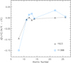 |
Fig. 4 NLTE corrections Δ[X/H] (NLTE − LTE) for the subgiant star Y923 (black triangles) and the turn-off star Y1388 (blue rectangles) as a function of atomic number. The corrections were calculated line by line relative to the Sun. |
Differential chemical abundances of our sample stars for 22 elements (24 species), relative to the Sun.
4 Discussion
In this section we discuss the elemental abundances of our programme stars, the effect of atomic diffusion, and the implications for chemicaltagging.
4.1 Elemental abundances of the subgiant stars in M 67
It is of particular interest to explore the elemental abundances of all our sample stars, and of the abundance variations within each stellar group. Figure 5 shows the elemental abundances of our subgiant stars (relative to the Sun) as a function of atomic number. In order to clarify the quantities of chemical homogeneity in the subgiant stars, we list the average elemental abundances, related dispersions (standard deviations of the mean), and the corresponding average errors for the subgiant stars in our sample for the 24 species in Table 4. We note that the dispersions are comparable to or smaller than the average errors for almost all the elements. The average elemental abundance of all the elements for the three subgiant stars in our sample is 0.074 dex, with an average dispersion of 0.016 dex, and an average error of 0.022 dex. Therefore, in spite of our small sample size, we would argue that the subgiant stars in our sample are chemically homogenous, also at a extremely high precision level (~0.02 dex).
4.2 Elemental abundances of turn-off stars in M 67
The elemental abundances of turn-off stars (relative to the Sun) in our sample as a function of atomic number is shown in Fig. 6. The average elemental abundances, related dispersions, and the average errors for the turn-off stars in our sample are listed in Table 4. It is clear that the variations in the elemental abundances in our turn-off stars are much larger than those of the subgiant stars. For the turn-off stars we find an average elemental abundance of −0.065 dex and an average dispersion in of 0.076 dex, while the average error is 0.023 dex. According to Table 4, all the species haveelemental abundance dispersions that are two to four times larger than the average errors.
At first glance, such a significant variation in elemental abundances in turn-off stars might be due to one outlier, Y2235. Y2235 has an overall metallicity of ≈0.04 dex, about 0.12 dex higher than that of Y1388 and 0.17 dex higher than that of Y535. However, we did not find any indications of binarity, for example an RV variation or visible double line feature from the spectrum of this star that could help explain the odd elemental abundances. Y2235 has a slightly cooler Teff and a slightly larger log g when compared to the other two turn-off stars. It is not likely that such a small difference in stellar parameters can cause such a large change in elemental abundance (>0.1 dex). We would have to decrease the Teff by about 150 K (seven timesthe uncertainty in Teff) or decrease the logg by about 0.2 dex (four times the uncertainty in logg) in order to force the metallicity of Y2235 to drop by about 0.1 dex, ignoring the impact of those changes on the excitation–ionization balance essential for obtaining the stellar parameters. Such a significant change would be neither realistic nor reasonable. In addition, by checking the spectrum, we note that Y2235 does have deeper spectral lines when compared to the two other turn-off stars (see Fig. 2). We cannot exclude the possibility that Y2235 has suffered some sort of mixing event related to planet engulfment. Since this is not the main scope of this paper, we only discuss briefly the planet-related scenarios in Appendix B.
We also found that the most metal-poor turn-off star, Y535, has a metallicity lower than Y1388 by about 0.05 dex (≲2 σ), although itsabundance behaviour seems similar to that of Y1388. This star has RV of ~20 km s−1, which is about 12 km s−1 lower than the average RV of the other programme stars. This indicates that Y535 might have a wide binary companion, although it is difficult to estimate how this companion would affect the chemical composition of Y535.
Because all three turn-off stars have a high probability of being members of M 67, our results imply that the turn-off stars in M 67 are chemically inhomogeneous. This phenomenon has been reported for main sequence dwarf stars in the Hyades (Liu et al. 2016a) and in the Pleiades (Spina et al. 2018), although these results were explained using different scenarios. Further discussion about abundance trends versus dust condensation temperature for our results are presented in Appendix B.
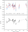 |
Fig. 5 Top panel: elemental abundances of our subgiant stars as a function of atomic number; black, blue, and red triangles represent the elemental abundances of Y519, Y923, and Y1844, respectively. Bottom panel: similar to the top panel, but for the average abundances of the subgiant stars (black filled triangles). The error bars represent the standard deviations of the mean values. |
4.3 Comparison to the previous studies of M 67
Before discussing the implications of our results, we compare our results to the previous spectroscopic studies of M 67. First, we compare our results to those from Gao et al. (2018)6 for the twostars in common, Y1844 (subgiant) and Y1388 (turn-off), and to that from Souto et al. (2018)7 for the one subgiant star we have in common, Y1844 (see Fig. 7). For Y1844 our derived elemental abundances for elements in common are more metal rich by 0.057 ± 0.027 (σ = 0.065) dex and 0.045 ± 0.010 (σ = 0.033) dex when compared to those from Gao et al. (2018) and Souto et al. (2018), respectively. For Y1388, our elemental abundances for common elements are also more metal rich than those from Gao et al. (2018) by 0.056 ± 0.018 (σ = 0.044) dex. For the individual stars our results agree with these two studies within the errors since the typical errors in the elemental abundances are ~0.05–0.1 dex in the two studies we used for comparison.
Second, we compared the average elemental abundance values of our stars to those from Önehag et al. (2014), Gao et al. (2018), and Souto et al. (2018) for the subgiant and turn-off stars separately (see Fig. 8). We found that the average elemental abundance values for the subgiant stars in our study are higher by about 0.06, 0.08, and 0.05 dex when compared to the values from Gao et al. (2018) and Souto et al. (2018). In addition, the average elemental abundance value for the turn-off stars in this study is slightly lower than that from Önehag et al. (2014) by about 0.03 dex, similar to that from Gao et al. (2018), and lower than that from Souto et al. (2018) by about 0.02 dex. We note that the average difference in elemental abundances between the subgiant and turn-off stars in our study is ≈ 0.07–0.08 dex higher compared to the two previous studies. Such a difference in elemental abundance between subgiant and turn-off stars is marginally comparable when taking into account the measurement uncertainties (and abundance scatters). The difference mainly originates from the quality of spectra and the level of uncertainties, as well as the selection of stars. For example, compared to the sample of our subgiant stars, the subgiants selected in Önehag et al. (2014) have in general similar log g values, but temperatures ~400 K higher. Therefore, their subgiants are located on an earlier stage of the stellar evolutionary track, which partly explains why the abundance difference reported in their study is smaller.
In general, our results clearly revealed the existence of abundance differences between the subgiant stars and the turn-off stars, where the subgiant stars are more metal-rich than the turn-off stars, although the observed abundance differences in this study (0.1–0.2 dex) are larger with higher significance than the previous spectroscopic studies. We recall that the typical uncertainty in abundance for individual stars from our study is ~0.02 dex, while the typical errors in abundances are between 0.05–0.15 dex in the previous studies (e.g. Önehag et al. 2014; Gao et al. 2018; Souto et al. 2018, 2019; Bertelli Motta et al. 2018).
4.4 Effects of atomic diffusion on derived elemental abundances
As noted in the introduction, atomic diffusion can cause surface abundances to vary as a function of stellar evolutionary phase. The maximum effect is seen near the turn-off point. As the star evolves from the turn-off point to the subgiant and red giant branches, the surface abundances return to nearly their original values due to the deepening of the surface convection zone.
From this study, we see that the subgiant stars in our sample are chemically homogeneous, to a high precision level (≈ 0.02 dex). Since the convection zones of subgiant stars are deep, any signatures of diffusion might be washed away. It is therefore also likely that the chemical composition of these stars is the closest to that of the primordial composition of the cluster based on this study. We note that the turn-off stars in our sample show large abundance variations (0.1–0.2 dex), implying that they are likely chemically inhomogeneous; the turn-off stars have the thinnest convective envelopes and diffusion has had the whole time of the main sequence evolution to affect their surface abundances, thus making their surface abundances variable. This might lead to the observed large abundance variations between the turn-off stars from our sample. We therefore suspect that the turn-off stars in M 67 might show the largest chemical inhomogeneity when compared to other stellar groups.
In order to test the effect of atomic diffusion in M 67, we compared our observational results to the stellar evolutionary models from Dotter et al. (2017) and O. Richard (priv. comm.). In Figs. 9–12, we show the elemental abundances for all the species analysed in this study, and for the values of solar twin Y1194. We then overplotted the values predicted by the model for those species which have been modelled. The adopted MIST models include overshooting mixing, turbulent diffusion and atomic diffusion, and radiative accelerations were included on an element-by-element basis. The elemental abundances predicted by the model were derived for solar metallicity (Asplund et al. 2009), initial mass ranging from 0.7 M⊙ to 1.4 M⊙, and ages of t = 4.0 Gyr and t = 5.0 Gyr. The model from O. Richard has taken into account atomic diffusion, but without additional mixing. The abundances predicted by his model were based on an age of ~3.7 Gyr and solar metallicity slightly differ (~ + 0.06 dex) from the value adopted by MIST models. We shifted the zero-point of the model predicted values to fit the results for the solar twin Y1194. We note that there are subtle differences between different models, but they agree in general.
For all elements, the relative elemental abundance ratios between the solar twin, the turn-off, and subgiant stars qualitatively matches the model. The turn-off stars have, on average, lower [X/H] than the solar twin, while the subgiant stars have, on average, higher [X/H] ratios than the solar twin. We note that our conclusion regarding diffusion does not hinge on a particular star such as the outlier Y2235. The best agreement between model predictions and observations occurs for oxygen. For other elements, the observed abundance differences are in general larger than the model predictions. We note that radiative levitation and turbulent mixing were taken into account for the models. Both of them have the effect of reducing the diffusion signatures in the turn-off stars. It has generally been found that a small amount of surface mixing, namely turbulent mixing, is required to match observations because the amount of depletion predicted by stellar models with diffusion but without any other mixing is too large. However, this extra mixing at the surface has not been completely tested by any means and not well justified physically. A physically motivated treatment of turbulent mixing in the surface layers would help in this regard. More observational results with high precision for the stars throughout the whole evolutionary stage are needed to better constrain or quantify the exact amount of turbulent mixing.
Average abundances, related dispersions (standard deviations of the mean), and the corresponding average errors for the subgiant stars and turn-off stars in our sample for 24 species, relative to the Sun.
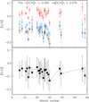 |
Fig. 6 Top panel: elemental abundances of the turn-off stars in our sample as a function of atomic number (black, blue, and red rectangles represent the abundances of Y535, Y1388, and Y2235, respectively). Bottom panel: similar to the top panel, but for the average elemental abundances of the turn-off stars (black filled rectangles). The error bars represent the standard deviations of the mean values. |
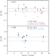 |
Fig. 7 Comparison of our results with those from Gao et al. (2018) and Souto et al. (2018) for the two stars in common. Top panel: comparison of elemental abundances of the subgiant star Y1844 (black, blue, and red triangles represent the results fromthis work, Gao et al. 2018, and Souto et al. 2018, respectively). Bottom panel: comparison of elemental abundances of the turn-off star Y1388 (black and blue rectangles represent the results from this work and Gao et al. 2018, respectively). The dashed lines represent the locations of mean elemental abundances from the corresponding studies. |
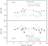 |
Fig. 8 Comparison of our results with those from Önehag et al. (2014), Gao et al. (2018), and Souto et al. (2018) for the average elemental abundances for subgiant and turn-off stars. Top panel: comparison of the average elemental abundances for the subgiant stars. Bottom panel: comparison of the average elemental abundances for the turn-off stars (black, green, blue, and red symbols represent the results from this work, Önehag et al. 2014, Gao et al. 2018, and Souto et al. 2018, respectively). |
4.5 Age and initial metallicity of M 67
As mentioned in Sect. 1, M 67 is an open cluster with near solar metallicity and an age of about 4 Gyr (VandenBerg et al. 2007; Yadav et al. 2008; Sarajedini et al. 2009; Önehag et al. 2011, 2014). Numerous theoretical studies by VandenBerg et al. (2006), Magic et al. (2010), Bressan et al. (2012), and Choi et al. (2016), among others, made use of M 67 to calibrate the efficiency of convective overshoot mixing in low-mass stars. The age estimation of M 67 could benefit from the high-precision stellar spectroscopic parameters derived in a strictly differential approach. Önehag et al. (2011) estimated the age of solar twin Y1194 in M 67 to be 4.2 ± 1.6 Gyr by fitting stellar evolutionary tracks using the Victoria stellar evolutionary code (based on VandenBerg et al. 2007) to their accurately determined stellar spectroscopic parameters.
In this study, we tried to fit the isochrones to our spectroscopic parameters for further exploration and verification. Figure 13 shows our results compared to a set of MIST isochrones with initial metallicities of [Fe/H] between 0 and 0.1, and age of 4 and 4.5 Gyr (Dotter 2016; Choi et al. 2016). The values of spectroscopic log g of our sample stars seem slightly higher than the values from MIST models by ~0.05 dex, but they arestill marginally comparable considering the uncertainties from observations and from theoretical models. It is difficult to tell which isochrone provides the best fit. We would argue, for the isochrones with an age of 4 Gyr, that [Fe/H] = +0.05 shows a good match for the two hottest stars, while the other stars clearly lie nearer to [Fe/H] = 0.1; instead, for the isochrones with an age of 4.5 Gyr, [Fe/H] = 0 shows a better match than [Fe/H] = 0.05 and 0.1. It has been suggested by Önehag et al. (2014) that the diffusion-corrected initial metallicity of M 67 is estimated to be [Fe/H] = 0.06. In this study, the average [Fe/H] of the subgiant stars in M 67 is ~0.07 dex. Based on our observational results in combination with the comparison with the theoretical isochrones, we estimate that the initial chemical composition of M 67 is probably between 0.05 and 0.1. Nevertheless, Choi et al. (2018) discussed the theoretical uncertainties in the model-based Teff scale. It is entirely possible that our Teff scale and that of the models differ by some small amount (~25–50 K), and this could cause a significant difference in the conclusion of which initial metallicity is to be preferred. In addition, the difference between different theoretical isochrones (e.g. MIST, PARSEC, and YY) would also affect the conclusion of the initial chemical composition of M 67.
Another method used to estimate the stellar ages is using [Y/Mg] abundance ratios. Nissen (2015, 2016) found that [Y/Mg] ratios correlate strongly with stellar ages for the solar twins and such abundance ratios can be used as a “chemical clock”. The empirical relation between [Y/Mg] and age was presented in these two studies. Feltzing et al. (2017) confirmed the relation for dwarfs of solar metallicity, but found that it disappears for stars with [Fe/H] ~−0.5 dex and below. Slumstrup et al. (2017) claimed that the empirical relation between [Y/Mg] and age as presented by Nissen (2016) was found to hold also for helium-core-burning giants of close to solar metallicity.
In this study we derived the chemical age of a solar twin Y1194 in M 67, using the [Y/Mg] ratio and the relation proposed by Nissen (2016). We found the chemical age of Y1194 to be: 4.15 ± 0.59 Gyr. This agrees well with the age estimation using isochrone fitting to our results and with that from Önehag et al. (2011). However, for the turn-off and subgiant stars in our sample, the chemical ages were found to be about 1.5 Gyr higher than that of the solar twin Y1194. The [Y/Mg] ratio in average is approximately −0.03 dex for our sample stars, agree well with that from Önehag et al. (2014) (approximately −0.04 dex); however, this is lower than the value for a giant star in M 67 (see Fig. 3, Slumstrup et al. 2017). Therefore, we suspect that the empirical relation between [Y/Mg] and age might not work well for the turn-off and subgiant stars.
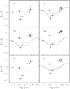 |
Fig. 9 Elemental abundances of C, O, Na, Mg, Al, and Si for our sample stars. The black and green dashed lines represent the model predictions with solar metallicity and at an age of 4.0 and 5.0 Gyr, respectively (Dotter et al. 2017). The red dotted line represents the model predictions by O. Richard (priv. comm.). Open triangles and rectangles represent the elemental abundances for the subgiant and turn-off stars, respectively. The solar twin Y1194 is shown as an open circle. |
4.6 Implications for chemical tagging
A basic assumption for chemical tagging to work is that open clusters, which are surviving star-forming aggregates in the Galactic disc, should be chemically homogeneous (Bland-Hawthorn et al. 2010; Blanco Cuaresma et al. 2015; De Silva et al. 2015; Ting et al. 2015).Determining the level of chemical homogeneity in open clusters is thus of fundamental importance to studying the evolution of star-forming clouds and that of the Galactic disc (Bovy 2016).
In the current study, we focus on the type of stars that are the prime targets for chemical tagging: dwarf stars on the main sequence, around the turn-off, and stars on the subgiant branch. Ideally, stars in these different evolutionary phases should have, if they formed from a single chemically homogenous star-forming event, the same elemental abundances. Our target stars have a high probability of being members of the old open cluster M 67.
We find that basically all elemental abundances in M 67 vary as a function of evolutionary stage of the star. This can be seen in Fig. 9–12, where we show the elemental abundances as a function of the surface gravity of the stars. The main sequence star in the sample has essentially solar elemental abundances, stars at the turn-off dip abut 0.1 dex below solar values (but note the one star that differs, see discussion in Sect. 4.4), while the subgiant stars again rise to super-solar values. Our study is of a highly differential nature, reaching high precision in the elemental abundances. A similar precision is rarely if ever reached in large spectroscopic catalogues such as the Gaia-ESO survey (Gilmore et al. 2012), the GALAH survey (De Silva et al. 2015), and the APOGEE survey (Majewski et al. 2017), due to the lower quality spectra (relative to our study).
From this study, we find that the subgiant stars in our sample are chemically homogeneous, under a high precision level (≈ 0.02 dex). As discussed in Sect. 4.4 we expect stars in this evolutionary phase to have well-mixed atmospheres and they are thus likely to have chemical compositions close to the primordial composition of the cluster ([Fe/H] ~ 0.05–0.1). This makes subgiant stars ideal targets for the application of the chemical tagging technique. We find that our turn-off stars show large abundance variations (0.1–0.2 dex). Again as discussed in Sect. 4.4, this is likely because diffusion has had the whole time of the main sequence evolution to act on their surface abundances, and on their thin convective envelopes, leading to the large variations in elemental abundances inside this group of stars. If this is true, then turn-off stars are probably not ideal targets for the chemical tagging technique and the purpose of Galactic archeology, unless the effects of atomic diffusion can be accurately corrected.
We note that this work is limited by the small number of stars studied. A high-precision differential abundance analysis on more M 67 members (especially turn-off stars) is necessary to probe and test the possible chemical inhomogeneity in the M 67 turn-off stars. Still, we believe that some general comments on which stars to choose for chemical tagging may already be done now (keeping in mind that we have not yet probed the chemical homogeneity of the main sequence stars). First, it would appear that sticking to one type of star might be highly advantageous if we want to find stars formed from the same star formation event, and that the best type of star appears to be the subgiant stars in our study. This is a sub-optimum conclusion as subgiant stars are, due to the short duration of this stellar evolutionary phase, relatively rare stars (e.g. see Fig. 1). Technically, it should be possible to correct the elemental abundances for the turn-off stars to reflect initial composition of the star-forming event; however, given the as yet limited number of models and knowledge about how the exact mixture of different elements in the atmosphere influences processes like diffusion, such corrections would at best have rather poor precision, which would mean that the corrected elemental abundances are not good enough for chemical tagging to work.
5 Conclusions
We presented a strictly line-by-line differential chemical abundance analysis of three turn-off stars and three subgiants in M 67 in order to confirm and quantify more precisely the effect of atomic diffusion in this old benchmark open cluster. Our targets are all members of M 67, at a high level of probability, according to Yadav et al. (2008) and Gaia Collaboration (2018). We obtained high-precision (~0.02 dex) relative abundance measurements for 22 elements for the sample stars.
Firstly, we found that the subgiant stars in our sample are chemically homogenous at a level of 0.02 dex, with an average elemental abundance of 0.074 dex, an abundance dispersion of 0.016 dex, and an average error on the elemental abundances of 0.022 dex. These stars are mirrors reflecting closely the original chemical composition of the open cluster, making them ideal targets for the application of chemical tagging. Secondly, we note that the turn-off stars in our sample show significant variations in the elemental abundances, with an average elemental abundance of −0.065 dex, with an average dispersion of 0.076 dex, and an average error in elemental abundance of 0.023 dex. Our results imply that the turn-off stars in our sample are likely chemically inhomogeneous, possibly due to the influence of turbulent mixing and diffusion in their interiors. If confirmed by future studies, this poses a major challenge to the concept of chemical tagging when using the turn-off stars as tracers or a mixture of stars from different evolutionary stages. Finally, we clearly showed that overall the subgiant stars are more metal rich than the turn-off stars by more than 0.1 dex, higher than the findings from previous spectroscopic studies. The relative elemental abundances for the solar twin, turn-off, and subgiant stars are qualitatively in agreement with stellar models that include atomic diffusion. We also find that the amplitude of the differences between the turn-off and subgiant stars is larger than the model predictions. Our results indicate that the effect of atomic diffusion, resulting in changes in surface abundances of stars during the different evolutionary phases, is prominent and should be taken into account when applying the chemical tagging technique to track the stars at different evolutionary stages.
Again, we note that the results reported here are based on a small number of stars. The most urgent action is now to extend the sample of stars studied in this way in M 67 and in a few selected open clusters with somewhat different properties (higher and lower iron abundances and lower ages) to further strengthen the empirical evidence for the size of atomic diffusion on final derived elemental abundances and to probe the level of chemical (in)homogeneity in the open cluster.
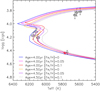 |
Fig. 13 Stellar spectroscopic parameters (Teff and log g) of our programme stars. The open circle, open rectangles, and open triangles correspond to our targets: solar twin Y1194, turn-off stars, and subgiant stars, respectively. The solar value is indicated by a red star. A set of MIST isochrones with initial metallicities of [Fe/H] between 0 and 0.1, and age of 4 and 4.5 Gyr (Dotter 2016; Choi et al. 2016) are shown as solid lines. |
Acknowledgements
F.L. and S.F. acknowledge support by the grant “The New Milky Way” from the Knut and Alice Wallenberg Foundation and the grant 184/14 from the Swedish National Space Agency. F.L. was also supported by the Märta and Eric Holmberg Endowment from the Royal Physiographic Society of Lund. This work has been supported by the Australian Research Council (grants FL110100012, FT140100554, and DP120100991). Parts of this research were conducted by the Australian Research Council Centre of Excellence for All Sky Astrophysics in 3 Dimensions (ASTRO 3D), through project number CE170100013. J.M. acknowledges support by FAPESP (2018/04055-8). We acknowledge valuable discussions with Dr. Ross Church. We thank the referee for the suggestions and comments that helped us to improve our manuscript. The authors thank the ANU Time Allocation Committee for awarding observation time to this project. The authors wish to acknowledge the very significant cultural role and reverence that the summit of Mauna Kea has always had within the indigenous Hawaiian community. We are most fortunate to have the opportunity to conduct observations from this mountain.
Appendix A Supplementary material
Table A.1 is only available at the CDS. It lists the atomic line data and the measured equivalent widths used for our analysis.
Appendix B Elemental abundances versus Tcond
Meléndez et al. (2009) conducted a high-precision differential abundance analysis for the Sun and the solar twins. They found that the Sun is depleted in refractory elements (with high Tcond) when compared to the majority (≈85%) of solar twins. The observed abundance differences correlate with Tcond, and were attributed to the influence of terrestrial planet formation. With a large sample, Bedell et al. (2018) confirmed that the Sun indeed has a special abundance pattern when compared to the other Sun-like stars. However, the hypothesis proposed by Meléndez et al. (2009) for the solar abundance pattern is still under debate. Adibekyan et al. (2014) and Nissen (2015) claimed that the detected abundances versus Tcond trends might be due to the effect of Galactic chemical evolution. Another possible scenario, namely “dust-cleansing”, suggested that the Sun was born in a dense environment where some of the dust in the proto-solar nebula was radiatively cleansed by luminous hot stars before the formation of the Sun, and left its refractory elemental abundances deficient. This was proposed and discussed by Önehag et al. (2011, 2014) for their studies on M 67 stars, where they found the M 67 stars have a chemical composition closer to solar composition than most solar twins. Their results indicate that the star-forming location and environment might play an important role in explaining the solar abundance pattern.
It is therefore of interest to examine the abundances versus Tcond trends for our sample stars. In Figs. B.1–B.6 we show the differential elemental abundances relative to the Sun as a function of Tcond8. We found that the slopes of [X/H] versus Tcond are positive with > 2 σ significance level for two subgiant stars (Y923 and Y1844), and relatively flat for one subgiant star (Y519). The slopes of [X/H] versus Tcond for two turn-off stars (Y1388 and Y2235) are flat, while negative with about 2.5σ significance level for one turn-off star (Y535). Because of the relatively large scatters in the [X/H] versus Tcond plots, we cannot identify any chemical signatures due to planet formation. We note that the abundance behaviours of our sample stars agree well with those from Önehag et al. (2014), and slightly favour the dust-cleansing hypothesis proposed in their study.
Considering that our turn-off stars are likely not chemically homogeneous, we examined the detailed abundance differences between these three turn-off stars. We show the differential elemental abundances of Y2235 and Y535 relative to Y1388 (the turn-off star with medium metallicity), as a function of Tcond in Figs. B.7 and B.8. We find that the slope of Δ[X/H] versus Tcond is almost flat when compared Y535 to Y1388, while the corresponding slope is positive with 2.4 σ significance level when compared Y2235 to Y1388. The phenomena are similar to the findings by Spina et al. (2018), who found trends with condensation temperature in the differential abundances of Pleiades stars, and suggested a possible connection with planets.
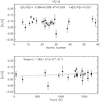 |
Fig. B.1 Top panel: differential abundances of subgiant star Y519 relative to the Sun as a function of atomic number. Bottom panel: differential abundances of Y519 relative to the Sun as a function of Tcond; the blue dashed line represents the linear least-squares fit to the data and the red dotted line represents the Tcond trend taken from Meléndez et al. (2009). |
References
- Adibekyan, V. Z., González Hernández, J. I., Delgado Mena, E., et al. 2014, A&A, 564, L15 [NASA ADS] [CrossRef] [EDP Sciences] [Google Scholar]
- Amarsi, A. M., Asplund, M., Collet, R., & Leenaarts, J. 2016, MNRAS, 455, 3735 [NASA ADS] [CrossRef] [Google Scholar]
- Asplund, M., Grevesse, N., Sauval, A. J., & Scott, P. 2009, ARA&A, 47, 481 [NASA ADS] [CrossRef] [Google Scholar]
- Battistini, C., & Bensby, T. 2015, A&A, 577, A9 [NASA ADS] [CrossRef] [EDP Sciences] [Google Scholar]
- Bedell, M., Bean, J. L., Meléndez, J., et al. 2018, ApJ, 865, 68 [NASA ADS] [CrossRef] [Google Scholar]
- Bensby, T., Feltzing, S., Lundström, I., & Ilyin, I. 2005, A&A, 433, A185 [NASA ADS] [CrossRef] [EDP Sciences] [Google Scholar]
- Bensby, T., Feltzing, S., & Oey, M. S. 2014, A&A, 562, A71 [NASA ADS] [CrossRef] [EDP Sciences] [Google Scholar]
- Bergemann, M. 2011, MNRAS, 413, 2184 [NASA ADS] [CrossRef] [Google Scholar]
- Bergemann, M., Lind, K., Collet, R., Magic, Z., & Asplund, M. 2012, MNRAS, 427, 27 [NASA ADS] [CrossRef] [Google Scholar]
- Bergemann, M., Kudritzki, R.-P., Würl, M., et al. 2013, ApJ, 764, 115 [NASA ADS] [CrossRef] [Google Scholar]
- Bergemann, M., Kudritzki, R.-P, Gazak, Z., Davies, B., & Plez, B. 2015, ApJ, 804, 113 [NASA ADS] [CrossRef] [Google Scholar]
- Bertelli Motta, C., Pasquali, A., Richer, J., et al. 2018, MNRAS, 478, 425 [NASA ADS] [CrossRef] [Google Scholar]
- Blanco-Cuaresma, S., Soubiran, C., Heiter, U., et al. 2015, A&A, 577, A47 [NASA ADS] [CrossRef] [EDP Sciences] [Google Scholar]
- Bland-Hawthorn, J., Karlsson, T., Sharma, S., et al. 2010, ApJ, 721, 582 [NASA ADS] [CrossRef] [Google Scholar]
- Bovy, J. 2016, ApJ, 817, 49 [NASA ADS] [CrossRef] [Google Scholar]
- Bressan, A., Marigo, P., Girardi, L., et al. 2012, MNRAS, 427, 127 [NASA ADS] [CrossRef] [Google Scholar]
- Castelli, F., & Kurucz, R. L. 2003, IAU Symp., 210, 20 [Google Scholar]
- Choi, J., Dotter, A., Conroy, C., et al. 2016, ApJ, 823, 102 [NASA ADS] [CrossRef] [Google Scholar]
- Choi, J., Dotter, A., Conroy, C., & Ting, Y. 2018, ApJ, 860, 131 [NASA ADS] [CrossRef] [Google Scholar]
- De Silva, G. M., Sneden, C., Paulson, D. B., et al. 2006, AJ, 131, 455 [NASA ADS] [CrossRef] [Google Scholar]
- De Silva, G. M., Freeman, K., Asplund, M., et al. 2007, AJ, 133, 1161 [NASA ADS] [CrossRef] [Google Scholar]
- De Silva, G. M., Freeman, K., Bland-Hawthorn, J., et al. 2015, MNRAS, 449, 2604 [NASA ADS] [CrossRef] [MathSciNet] [Google Scholar]
- Dotter, A. 2016, ApJS, 222, 8 [NASA ADS] [CrossRef] [Google Scholar]
- Dotter, A., Conroy, C., Cargile, P., & Asplund, M. 2017, ApJ, 840, 99 [NASA ADS] [CrossRef] [Google Scholar]
- Epstein, C. R., Johnson, J. A., Dong, S., et al. 2010, ApJ, 709, 447 [NASA ADS] [CrossRef] [Google Scholar]
- Feltzing, S., Howes, L. M., McMillan, P. J., & Stonkute, E. 2017, MNRAS, 465, L109 [NASA ADS] [CrossRef] [Google Scholar]
- Feng, Y., & Krumholz, M. R. 2014, Nature, 513, 523 [NASA ADS] [CrossRef] [Google Scholar]
- Freeman, K., & Bland-Hawthorn, J. 2002, ARA&A, 40, 487 [NASA ADS] [CrossRef] [Google Scholar]
- Gaia Collaboration (Brown A. G. A., et al.) 2018, A&A, 616, A1 [NASA ADS] [CrossRef] [EDP Sciences] [Google Scholar]
- Gao, X., Lind,K., Amarsi, A. M., et al. 2018, MNRAS, 481, 2666 [NASA ADS] [CrossRef] [Google Scholar]
- Gilmore, G., Randich, S., Asplund, M., et al. 2012, The Messenger, 147, 25 [NASA ADS] [Google Scholar]
- Grevesse, N., Scott, P., Asplund, M., & Sauval, A. J. 2015, A&A, 573, A27 [NASA ADS] [CrossRef] [EDP Sciences] [Google Scholar]
- Gruyters, P., Korn, A. J., Richard, O., et al. 2013, A&A, 555, A31 [NASA ADS] [CrossRef] [EDP Sciences] [Google Scholar]
- Korn, A. J., Grundahl, F., Richard, O., et al. 2007, ApJ, 671, 402 [NASA ADS] [CrossRef] [Google Scholar]
- Kurucz, R., & Bell, B. 1995, Kurucz CD-ROM, NO. 23, Harvard-Smithsonian Centre for Astrophysics [Google Scholar]
- Lind, K., Korn, A. J., Barklem, P. S., & Grundahl, F. 2008, A&A, 490, 777 [NASA ADS] [CrossRef] [EDP Sciences] [Google Scholar]
- Lind, K., Asplund, M., Barklem, P. S., & Belyaev, A. K. 2011, A&A, 528, A103 [NASA ADS] [CrossRef] [EDP Sciences] [Google Scholar]
- Liu, F., Asplund, M., Ramírez, I, Yong, D., & Meléndez, J. 2014, MNRAS, 442, L51 [NASA ADS] [CrossRef] [Google Scholar]
- Liu, F., Yong, D., Asplund, M., Ramírez, I., & Meléndez, J. 2016a, MNRAS, 457, 3934 [NASA ADS] [CrossRef] [Google Scholar]
- Liu, F., Yong, D., Asplund, M., et al. 2016b, MNRAS, 456, 2636 [NASA ADS] [CrossRef] [Google Scholar]
- Liu, F., Asplund, M., Yong, D., et al. 2016c, MNRAS, 463, 696 [NASA ADS] [CrossRef] [Google Scholar]
- Lodders, K. 2003, ApJ, 591, 1220 [NASA ADS] [CrossRef] [Google Scholar]
- Magic, Z., Serenelli, A., Weiss, A., & Chaboyer, B. 2010, ApJ, 718, 1378 [NASA ADS] [CrossRef] [Google Scholar]
- Majewski, S. R., Schiavon, R. P., Frinchaboy, P. M., et al. 2017, AJ, 154, 94 [NASA ADS] [CrossRef] [Google Scholar]
- Meléndez, J., Asplund, M., Gustafsson, B., & Yong, D. 2009, ApJ, 704, L66 [NASA ADS] [CrossRef] [Google Scholar]
- Meléndez, J., Ramírez, I., Karakas, A. I., et al. 2014, A&A, 791, A14 [Google Scholar]
- Michaud, G., Fontaine, G., & Beaudet, G. 1984, ApJ, 282, 206 [NASA ADS] [CrossRef] [Google Scholar]
- Michaud, G., Alecian, G., & Richer, J. 2015, Atomic Diffusion in Stars, Astronomy and Astrophysics Library (Cham: Springer) [CrossRef] [Google Scholar]
- Nissen, P. E. 2015, A&A, 579, A52 [NASA ADS] [CrossRef] [EDP Sciences] [Google Scholar]
- Nissen, P. E. 2016, A&A, 593, A65 [NASA ADS] [CrossRef] [EDP Sciences] [Google Scholar]
- Nordlander, T., & Lind, K. 2017, A&A, 607, A75 [NASA ADS] [CrossRef] [EDP Sciences] [Google Scholar]
- Nordlander, T., Korn, A. J., Richard, O., & Lind, K. 2012, ApJ, 753, 48 [NASA ADS] [CrossRef] [Google Scholar]
- Önehag, A., Korn, A. J., Gustafsson, B., Stempels, E., & VandenBerg, D. A. 2011, A&A, 528, A85 [NASA ADS] [CrossRef] [EDP Sciences] [Google Scholar]
- Önehag, A., Gustafsson, B., & Korn, A. J. 2014, A&A, 562, A102 [NASA ADS] [CrossRef] [EDP Sciences] [Google Scholar]
- Pasquini, L., Biazzo, K., Bonifacio, P., Randich, S., & Bedin, L. R. 2008, A&A, 489, 677 [NASA ADS] [CrossRef] [EDP Sciences] [Google Scholar]
- Prochaska, J. X., Naumov, S. O., Carney, B. W., McWilliam, A., & Wolfe, A. M. 2000, AJ, 120, 2513 [NASA ADS] [CrossRef] [Google Scholar]
- Ramírez, I., Asplund, M., Baumann, P., Meléndez, J., & Bensby, T. 2010, A&A, 521, A33 [NASA ADS] [CrossRef] [EDP Sciences] [Google Scholar]
- Sarajedini, A., Dotter, A., & Kirkpatrick, A. 2009, ApJ, 698, 1872 [NASA ADS] [CrossRef] [Google Scholar]
- Scott, P., Grevesse, N., Asplund, M., et al. 2015a, A&A, 573, A25 [NASA ADS] [CrossRef] [EDP Sciences] [Google Scholar]
- Scott, P., Asplund, M., Grevesse, N., et al. 2015b, A&A, 573, A26 [NASA ADS] [CrossRef] [EDP Sciences] [Google Scholar]
- Slumstrup, D., Grundahl, F., Brogaard, K., et al. 2017, A&A, 604, L8 [NASA ADS] [CrossRef] [EDP Sciences] [Google Scholar]
- Sneden, C. 1973, ApJ, 184, 839 [NASA ADS] [CrossRef] [Google Scholar]
- Sobeck, J. S., Kraft, R. P., Sneden, C., et al. 2011, AJ, 141, 175 [NASA ADS] [CrossRef] [Google Scholar]
- Souto, D., Cunha, K., Smith, V. V., et al. 2018, ApJ, 857, 14 [NASA ADS] [CrossRef] [Google Scholar]
- Souto, D., Allende Prieto, C., Cunha, K., et al. 2019, ApJ, 874, 97 [NASA ADS] [CrossRef] [Google Scholar]
- Spina, L., Meléndez, J., Casey, A. R., Karakas, A. I., & Tucci-Maia, M. 2018, ApJ, 863, 179 [NASA ADS] [CrossRef] [Google Scholar]
- Ting, Y. S., Conroy, C., & Goodman, A. 2015, ApJ, 807, 104 [NASA ADS] [CrossRef] [Google Scholar]
- VandenBerg, D. A., Bergbusch, P. A., & Dowler, P. D. 2006, ApJS, 162, 375 [NASA ADS] [CrossRef] [MathSciNet] [Google Scholar]
- VandenBerg, D. A., Gustafsson, B., Edvardsson, B., Eriksson, K., & Ferguson, J. 2007, ApJ, 666, L105 [NASA ADS] [CrossRef] [Google Scholar]
- Vogt, S. S., Allen, S. L., Bigelow, B. C., et al. 1994, SPIE, 2198, 362 [Google Scholar]
- Yadav, R. K. S., Bedin, L. R., Piotto, G., et al. 2008, A&A, 484, 609 [NASA ADS] [CrossRef] [EDP Sciences] [Google Scholar]
IRAF is distributed by the National Optical Astronomy Observatory, which is operated by Association of Universities for Research in Astronomy, Inc., under cooperative agreement with National Science Foundation.
These two spectra were used in our previous study (Liu et al. 2016c), but re-analysed in this study for comparison and consistency purposes.
All the corrections were made line by line, differentially relative to the Sun.
We adopted their NLTE results for all the common elements.
Only LTE results are available and thus being adopted.
50% Tcond of each element was taken from Lodders (2003).
All Tables
Adopted solar parameters and derived stellar parameters for our programme stars (relative to the Sun).
Differential chemical abundances of our sample stars for 22 elements (24 species), relative to the Sun.
Average abundances, related dispersions (standard deviations of the mean), and the corresponding average errors for the subgiant stars and turn-off stars in our sample for 24 species, relative to the Sun.
All Figures
|
Fig. 1 Our programme stars in the colour magnitude diagram, selected from Yadav et al. (2008), all with a high probability of membership. The red symbols correspond to our targets: solar twin Y1194 (red circle), turn-off stars (red rectangles), subgiant stars (red triangles). The blue, magenta, and red solid lines correspond to the isochrones for an age of 4 Gyr, |
| In the text | |
|
Fig. 2 Top panel: portion of the reduced spectra for the subgiant stars in our sample; Y519, Y923, and Y1844 are plotted in black, blue, and red, respectively. A few atomic lines (Si I, Ti I, Fe I) used in our analysis in this region are marked by the dashed lines. Bottom panel: similar to the top panel, but for the turn-off stars in our sample; Y535, Y1388, and Y2235 are plotted in black, blue, and red, respectively. |
| In the text | |
|
Fig. 3 Top panel: [Fe/H] of Y923 derived on a line-by-line basis with respect to the Sun as a function of LEP; open circles and blue filled circles represent Fe I and Fe II lines, respectively. The black dotted line shows the location of mean [Fe/H], the green dashed line represents the linear least-squares fit to the data. Bottom panel: same as the top panel, but as a function of reduced equivalent width. |
| In the text | |
|
Fig. 4 NLTE corrections Δ[X/H] (NLTE − LTE) for the subgiant star Y923 (black triangles) and the turn-off star Y1388 (blue rectangles) as a function of atomic number. The corrections were calculated line by line relative to the Sun. |
| In the text | |
|
Fig. 5 Top panel: elemental abundances of our subgiant stars as a function of atomic number; black, blue, and red triangles represent the elemental abundances of Y519, Y923, and Y1844, respectively. Bottom panel: similar to the top panel, but for the average abundances of the subgiant stars (black filled triangles). The error bars represent the standard deviations of the mean values. |
| In the text | |
|
Fig. 6 Top panel: elemental abundances of the turn-off stars in our sample as a function of atomic number (black, blue, and red rectangles represent the abundances of Y535, Y1388, and Y2235, respectively). Bottom panel: similar to the top panel, but for the average elemental abundances of the turn-off stars (black filled rectangles). The error bars represent the standard deviations of the mean values. |
| In the text | |
|
Fig. 7 Comparison of our results with those from Gao et al. (2018) and Souto et al. (2018) for the two stars in common. Top panel: comparison of elemental abundances of the subgiant star Y1844 (black, blue, and red triangles represent the results fromthis work, Gao et al. 2018, and Souto et al. 2018, respectively). Bottom panel: comparison of elemental abundances of the turn-off star Y1388 (black and blue rectangles represent the results from this work and Gao et al. 2018, respectively). The dashed lines represent the locations of mean elemental abundances from the corresponding studies. |
| In the text | |
|
Fig. 8 Comparison of our results with those from Önehag et al. (2014), Gao et al. (2018), and Souto et al. (2018) for the average elemental abundances for subgiant and turn-off stars. Top panel: comparison of the average elemental abundances for the subgiant stars. Bottom panel: comparison of the average elemental abundances for the turn-off stars (black, green, blue, and red symbols represent the results from this work, Önehag et al. 2014, Gao et al. 2018, and Souto et al. 2018, respectively). |
| In the text | |
|
Fig. 9 Elemental abundances of C, O, Na, Mg, Al, and Si for our sample stars. The black and green dashed lines represent the model predictions with solar metallicity and at an age of 4.0 and 5.0 Gyr, respectively (Dotter et al. 2017). The red dotted line represents the model predictions by O. Richard (priv. comm.). Open triangles and rectangles represent the elemental abundances for the subgiant and turn-off stars, respectively. The solar twin Y1194 is shown as an open circle. |
| In the text | |
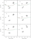 |
Fig. 10 Same as Fig. 9, but for S, Ca, Sc, Ti I, Ti II, and V. |
| In the text | |
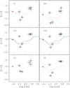 |
Fig. 11 Same as Fig. 9, but for Cr, Mn, Fe I, Fe II, Co, and Ni. |
| In the text | |
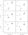 |
Fig. 12 Same as Fig. 9, but for Cu, Zn, Sr, Y, Ba, and Ce. |
| In the text | |
|
Fig. 13 Stellar spectroscopic parameters (Teff and log g) of our programme stars. The open circle, open rectangles, and open triangles correspond to our targets: solar twin Y1194, turn-off stars, and subgiant stars, respectively. The solar value is indicated by a red star. A set of MIST isochrones with initial metallicities of [Fe/H] between 0 and 0.1, and age of 4 and 4.5 Gyr (Dotter 2016; Choi et al. 2016) are shown as solid lines. |
| In the text | |
|
Fig. B.1 Top panel: differential abundances of subgiant star Y519 relative to the Sun as a function of atomic number. Bottom panel: differential abundances of Y519 relative to the Sun as a function of Tcond; the blue dashed line represents the linear least-squares fit to the data and the red dotted line represents the Tcond trend taken from Meléndez et al. (2009). |
| In the text | |
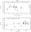 |
Fig. B.2 Same as Fig. B.1, but for subgiant star Y923 relative to the Sun. |
| In the text | |
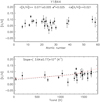 |
Fig. B.3 Same as Fig. B.1, but for subgiant star Y1844 relative to the Sun. |
| In the text | |
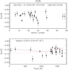 |
Fig. B.4 Same as Fig. B.1, but for turn-off star Y535 relative to the Sun. |
| In the text | |
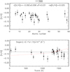 |
Fig. B.5 Same as Fig. B.1, but for turn-off star Y1388 relative to the Sun. |
| In the text | |
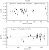 |
Fig. B.6 Same as Fig. B.1, but for turn-off star Y2235 relative to the Sun. |
| In the text | |
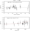 |
Fig. B.7 Same as Fig. B.1, but for Y535 relative to Y1388. |
| In the text | |
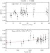 |
Fig. B.8 Same as Fig. B.1, but for Y2235 relative to Y1388. |
| In the text | |
Current usage metrics show cumulative count of Article Views (full-text article views including HTML views, PDF and ePub downloads, according to the available data) and Abstracts Views on Vision4Press platform.
Data correspond to usage on the plateform after 2015. The current usage metrics is available 48-96 hours after online publication and is updated daily on week days.
Initial download of the metrics may take a while.