| Issue |
A&A
Volume 599, March 2017
|
|
|---|---|---|
| Article Number | A141 | |
| Number of page(s) | 23 | |
| Section | Extragalactic astronomy | |
| DOI | https://doi.org/10.1051/0004-6361/201629802 | |
| Published online | 16 March 2017 | |
SDSS IV MaNGA: Deep observations of extra-planar, diffuse ionized gas around late-type galaxies from stacked IFU spectra⋆
1 Max-Planck Institute for Astrophysics, Karl-Schwarzschild-Str 1, 85748 Garching, Germany
e-mail: This email address is being protected from spambots. You need JavaScript enabled to view it.
2 Apache Point Observatory, PO Box 59, Sunspot, NM 88349, USA
3 Special Astrophysical Observatory of the Russian AS, 369167 Nizhnij Arkhyz, Russia
4 Space Telescope Science Institute, 3700 San Martin Drive, Baltimore, MD 21218, USA
5 Department of Astronomy, University of Wisconsin-Madison, 475N. Charter St., Madison WI 53703, USA
6 PITT PACC, Department of Physics and Astronomy, University of Pittsburgh, Pittsburgh, PA 15260, USA
7 Department of Physics and Astronomy, University of Utah, 115 S. 1400 E., Salt Lake City, UT 84112, USA
8 UCO/Lick Observatory, University of California, 1156 High St. Santa Cruz, Santa Cruz, CA 95064, USA
9 Center for Astrophysical Sciences, Department of Physics and Astronomy, Johns Hopkins University, 3400 North Charles Street, Baltimore, MD 21218, USA
10 Department of Physics and Astronomy, Bates College, Lewiston, ME 04240, USA
11 McDonald Observatory, The University of Texas at Austin, 1 University Station, Austin, TX 78712, USA
12 Departamento de Física, CCNE, Universidade Federal de Santa Maria, 97105-900, Santa Maria, RS, Brazil
13 Laboratório Interinstitucional de e-Astronomia-LInea, Rua Gal. José Cristino 77, 20921-400 Rio de Janeiro, Brazil
14 Instituto de Astronomia, Universidad Nacional Autónoma de México, A.P. 70-264, 04510 Mexico, D.F., Mexico
15 Institute of Cosmology & Gravitation, University of Portsmouth, Dennis Sciama Building, Portsmouth, PO1 3FX, UK
16 School of Physical Sciences, The Open University, Milton Keynes, MK1 15, UK
17 Department of Physics and Astronomy, University of Kentucky, 505 Rose Street, Lexington, KY 40506, USA
Received: 28 September 2016
Accepted: 8 December 2016
Abstract
We have conducted a study of extra-planar diffuse ionized gas using the first year data from the MaNGA IFU survey. We have stacked spectra from 49 edge-on, late-type galaxies as a function of distance from the midplane of the galaxy. With this technique we can detect the bright emission lines Hα, Hβ, [O ii]λλ3726, 3729, [O iii]λ5007, [N ii]λλ6549, 6584, and [S ii]λλ6717, 6731 out to about 4 kpc above the midplane. With 16 galaxies we can extend this analysis out to about 9 kpc, i.e. a distance of ~2Re, vertically from the midplane. In the halo, the surface brightnesses of the [O ii] and Hα emission lines are comparable, unlike in the disk where Hα dominates. When we split the sample by specific star-formation rate, concentration index, and stellar mass, each subsample’s emission line surface brightness profiles and ratios differ, indicating that extra-planar gas properties can vary. The emission line surface brightnesses of the gas around high specific star-formation rate galaxies are higher at all distances, and the line ratios are closer to ratios characteristic of H ii regions compared with low specific star-formation rate galaxies. The less concentrated and lower stellar mass samples exhibit line ratios that are more like H ii regions at larger distances than their more concentrated and higher stellar mass counterparts. The largest difference between different subsamples occurs when the galaxies are split by stellar mass. We additionally infer that gas far from the midplane in more massive galaxies has the highest temperatures and steepest radial temperature gradients based on their [N ii]/Hα and [O ii]/Hα ratios between the disk and the halo.
Key words: techniques: imaging spectroscopy / galaxies: halos / galaxies: evolution / galaxies: abundances / galaxies: spiral / galaxies: ISM
SDSS IV.
© ESO, 2017
1. Introduction
Ionized gas in the outskirts of galaxies has been the subject of study for several decades. In the Milky Way (MW), a layer of diffuse ionized gas (DIG) a few kpc above the plane of the galaxy (sometimes also referred to as a warm ionized medium (WIM) was discovered in the early 1970s and is commonly called the Reynolds Layer (Reynolds 1971; Reynolds et al. 1973). This layer contains most of the ionized gas in the MW, which is comparable (~30%) to the total mass of neutral hydrogen in the Galaxy (Reynolds 1990, 1991). More recently, several wide-angle surveys of MW Hα emission were combined by Finkbeiner (2003) to produce an all-sky map of Hα emission in the MW. Present practically everywhere, Hα emission contains much structure, such as loops, filaments, and blobs. Forbidden optical emission lines have also been studied. Similar to Hα, the luminosities of [S ii] and [N ii] vary spatially (e.g., Madsen et al. 2006). The ratios of [S ii] and [N ii] with respect to Hα are higher in the DIG compared to classic H ii regions, indicating that the properties of the DIG differ from those in H ii regions (e.g., Haffner et al. 2009).
Diffuse ionized gas has also been detected around other galaxies. Some of the first observations of diffuse gas in external galaxies were those of NGC 891 by Rand et al. (1990), Dettmar (1990). Hoopes et al. (1999) compared narrow-band Hα imaging of four nearby galaxies. They found that the Hα emission had substructure and that the Hα luminosity varied from galaxy to galaxy in their sample, with the more star-forming galaxies exhibiting stronger Hα emission. Lehnert & Heckman (1994) found that DIG was common in starforming galaxies. In face-on galaxies it was also seen that the DIG was correlated with H ii regions (e.g., Zurita et al. 2000, 2002). This work was followed up with a survey of 74 edge-on galaxies by Rossa & Dettmar (2003a,b) with a goal to understand how common Hα halos are around galaxies, as well as how the properties of these halos depend on star-formation rate. These authors found that Hα could be detected if the star-formation rate per unit area was above a threshold of 3.2 ± 0.5 × 1040 ergs-1kpc-2, with an estimated mean sensitivity for the galaxies observed with DFOSC at La Silla around 6 × 10-18 ergs-1 cm-2 arcsec-2 (Rand 1996).
In addition to narrow-band imaging, there have also been spectroscopic studies of nearby galaxies (Greenawalt et al. 1997; Hoopes & Walterbos 2003). The detection of multiple emission lines allows better constraints on a possible additional heating source, as well as the physical conditions of the extra-planar diffuse ionized gas (eDIG), such as its density and temperature. Radiation from OB stars escaping from the disk has been traditionally considered to be the main source of ionization (Haffner et al. 2009), however in some cases there is a need for an additional heating source beyond photoionization. Otte et al. (2001) studied the optical emission lines from [O ii]λ3727 to [S ii]λ6717 for three galaxies. All three galaxies had an [O ii]/Hα ratio that increased with distance from the galaxy midplane. Keeping the oxygen abundance constant while increasing the temperature as a function of radius yielded results in good agreement with the data. It is difficult to accommodate these results if only radiation from OB stars is considered; OB stars are confined to the disk and heating effects are expected to drop as a function of distance from the disk plane (however, see Wood et al. 2010; Barnes et al. 2014, for a contrasting view). Another possible additional heating source are hot, low-mass evolved stars (HOLMES) in the thick disk and stellar halo, which have been proposed to explain the emission line ratios in NGC 891 (Flores-Fajardo et al. 2011). Planetary nebulae and white dwarfs are hot and have a harder ionizing spectrum that could explain the observed emission line ratios, but it is unclear whether the density of such sources is high enough to maintain these temperatures at the required level. Other possible additional sources of heat in the diffuse halo gas are shocks (e.g., Collins & Rand 2001), photoelectric heating (Reynolds & Cox 1992), turbulence (e.g., Binette et al. 2009), and magnetic reconnection (e.g., Reynolds et al. 1999).
One of the main challenges in understanding the eDIG is to disentangle ionization from hot stars in the disk and other possible additional heating sources. This additional heating source may also depend on the galaxy mass or type, as seen in a study of irregular galaxies which have higher [O iii]/Hβ and lower [N ii]/Hα compared to spiral galaxies (Hidalgo-Gámez 2006). Finally, it is not yet understood whether the eDIG is inflowing, outflowing or simply in pressure-supported equilibrium around the galaxy. Inflowing gas from the circumgalactic medium (CGM) surrounding galaxies has been proposed to explain ongoing star-formation in spiral galaxies like the MW (White & Rees 1978). Inflowing gas is thought to come from gas that is cooling from the surrounding halo, or it may be recycled gas that is first ejected and then falls back onto the disk in the form of galactic fountains or chimneys (Putman et al. 2012, and references therein). Outflowing gas can be from galactic winds produced in supernovae explosions or from active galactic nuclei (AGN). Understanding the kinematics of the inflowing and outflowing gas around galaxies is key to understanding the processes that regulate star-formation in these systems. In a few studies (Heald et al. 2006a,b, 2007; Kamphuis et al. 2007), the outer regions of several galaxies, NGC 5775, NGC 891, and NGC 4302, were found to have negative velocity gradients with distance in the eDIG. These gradients were inconsistent with the ballistic model of Collins et al. (2002) for a star-formation driven disk-halo flow.
In a recent study, Ho et al. (2016) used the Sydney-AAO Multi-object Integral field spectrograph (SAMI) galaxy survey (Bryant et al. 2015) to study the eDIG of 40 galaxies. They only considered galaxies with a clear Hα detection in the outskirts, which limited their sample to galaxies with higher star-formation rates. They were interested in the connection between star-formation rates and galactic winds and they found higher amounts of eDIG in galaxies with a recent star-formation burst. They also detected emission lines (Hα, Hβ, [OI], [O ii], [O iii], [N ii], and [S ii]) out to ~10 kpc, however their galaxies are on average twice as large as the galaxies in our sample due to their higher median stellar mass. In our study we focus on how the average properties of the eDIG vary as a function of height above the disk and for galaxies with a range of properties.
Large IFU spectroscopic surveys, such as the Mapping Nearby Galaxies at Apache Point (MaNGA) survey, allow us to gain new and different perspectives on the eDIG. MaNGA will eventually obtain spectroscopic observations for 10000 nearby galaxies, with 1392 galaxies observed already in the first year. As we will show, a small, but significant fraction of these galaxies are edge-on, late-type systems for which it is possible to study the eDIG out to between approximately 4 and 9 kpc above and below the galactic plane. By stacking together spectra from similar galaxies, we can clearly detect emission lines farther out into the halo than previously possible due to the increased signal to noise for an average late-type galaxy. Previous very deep observations of NGC 891 and NGC 5775 have detections out to about 10kpc (Rand 1997, 2000). We can study how the properties of the emission lines depend on galaxy mass, morphological type, and specific star-formation rate. In this paper, we present results from the first year of observations. In Sect. 2 we describe the method for selecting our galaxy sample, our method for stacking the spectra, and our techniques for measuring emission line surface brightnesses and their associated errors. In Sect. 3, we present our main results for the full sample as well as for a sample in which it is possible to measure the radial profiles of the Hα and [O ii] lines out to ~9kpc. We also present results for several subsamples of galaxies which were selected according to specific star-formation rate, concentration index, and stellar mass. Finally, we conclude and summarize in Sect. 4.
In this paper, we refer to the ionized gas in the outskirts of galaxies as eDIG for simplicity, even though this ionized gas could also originate from outflows or shocks. The acronym DIG refers to the diffuse ionized gas that is present anywhere in the galaxy. We assume a Hubble constant H0 = 70kms-1 Mpc-1 throughout.
2. Method
In this section, we will first discuss the MaNGA survey and how we selected our galaxies (Sect. 2.1). We also show that our sample is representative of the late-type galaxies currently observed by MaNGA. We then discuss our stacking technique, including corrections and normalizations for each spectrum that is included into a stack, in Sect. 2.2. We also demonstrate the improvement to the achieved S/N by stacking. Lastly, in Sect. 2.3, we discuss the spectral fitting of the stacked spectra for extracting the emission line surface brightnesses.
2.1. Data set
We used the data from the SDSS-IV MaNGA survey (see Blanton et al. 2017, for an overview of SDSS-IV and for MaNGA Bundy et al. 2015). MaNGA began operations in 2014 and is a six year IFU survey of nearby galaxies. MaNGA uses the BOSS spectrographs, with a spectral range from 3622 to 10 354 Å and a resolution of R ~ 2000 (Smee et al. 2013). For this work we only used the wavelength range shortwards of 7000 Å, because sky residuals from the OH skylines limit the achievable depths in the outer low surface brightness regions of the galaxies at longer wavelengths (see Law et al. 2016).
The observations were taken with the 2.5 m Sloan Foundation telescope at Apache Point Observatory in New Mexico, USA (Gunn et al. 2006). Each observation is a plate containing 1423 fibers that are bundled into different sized units (Drory et al. 2015). For science purposes, there are five 127, two 91, four 61, four 37, and two 19 fiber bundles (Wake et al., in prep.). There are 12 seven-fiber bundles for observing spectrophotometric standard stars and 92 sky fibers for the sky background subtraction (Yan et al. 2016a). For the analysis presented in this paper, we mostly use the larger science bundles, because they typically have more fibers that extend to larger angular radii. The bundles are hexagonal in shape with the galaxy center at the origin (except in a few test cases which are not part of our sample). The list of plates and IFU bundles for each galaxy in our sample is provided in Table A.1. We note, that the IFU design number is the IFU bundle size followed by two digits signifying which IFU bundle of that size was used (so 12705 would be the fifth IFU bundle with 127 fibers).
The survey observes 2/3 of the galaxies out to a minimum radius of 1.5 effective radii (Re), known as the primary sample, and the remaining 1/3 out to 2.5 Re (secondary sample). The observational strategy is given in Law et al. (2015) and the first year survey data is described in Yan et al. (2016b). This targeting strategy enables a more comprehensive study of the outskirts of galaxies compared to other IFU surveys that do not have such a requirement (e.g., CALIFA; Sánchez et al. 2012). Each plate is observed in three different dithering positions multiple times, which are then reconstructed into a datacube. For our analysis we have used the row-stacked spectra instead of the data cube, which provides the spectra from each dithered position prior to the resampling. The data reduction pipeline was improved since SDSS III with better sky subtraction and less systemic residual flux which allows the stacking of low surface brightness spectra of many individual fibers without becoming dominated by background noise (Law et al. 2016).
We chose to study edge-on, late type galaxies. The constraint that the galaxies must be edge-on is valuable for two reasons. First, there is a greater area of the IFU that is in the halo of the galaxy. This also means that we are not limited to using galaxies only from the secondary sample. Second, studying the emission perpendicular to the plane of the disk minimizes contamination from gas and stars within the disk itself. We require the ratio of the semi-minor to semi-major axis (b/a) to be less than 0.3. This cutoff is similar to the one in Ho et al. (2016) with a cutoff of b/a < 0.26.
In this study we are interested in studying late-type systems with as wide a range of stellar masses (Mstar), star-formation rates, and morphologies as possible. We define a late-type galaxy as having a concentration index C (defined as the ratio R90/R50, where R90 and R50 are the radii enclosing 90% and 50% of the total r-band light from the galaxy) less than 2.6 (Shimasaku et al. 2001). Shimasaku et al. (2001) show that this is a robust way to separate late and early type galaxies even for highly inclined systems. According to this definition there are 81 galaxies with b/a < 0.3 in the entire first year sample. Six of these galaxies have an effective radius (Re) that appears to be wrongly measured or overly influenced by a bright bulge, one is a galaxy merger, 17 have another object (e.g., a star) in the field of view, and five show asymmetries along the disk, so they are discarded. We also required there to be fibers out to at least 4kpc above the disk midplane, which excludes another three galaxies. This leaves us with a total sample of 49 galaxies, which we call the full sample. Another sample, called the large-z sample, consists of galaxies with fibers simultaneously out to at least 9 kpc and 2 Re along the minor axis. We relaxed the b/a restriction to b/a < 0.4, which added four more galaxies. We also required that b/a × Re be less than 2 kpc, which limits the apparent height of the disk, to ensure that the outer stacks are coming from the halo and not a mixture of disk and halo. In total, there are 16 galaxies in this sample. As the survey continues, the number of galaxies suitable for this study will increase, allowing for a more detailed analysis of the extra-planar, diffuse ionized gas.
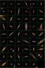 |
Fig. 1 SDSS images of all the galaxies used in the analysis. The images are in the same order as Table A.1 (left to right, then top to bottom). Each box is 60 × 60 arcsec with the centers corresponding to the coordinates given in Table A.1. The four additional galaxies for the large-z sample are also included as the last four galaxies. |
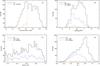 |
Fig. 2 Histograms showing the distributions of the MaNGA first year sample (black) and our sample of galaxies (orange) for various galactic properties. Panel a) shows the distribution of concentration index C with the vertical dashed purple line showing the division between late-type and early-type galaxies at C = 2.6. Panel b) gives the Mstar for the full sample (black), late-type galaxies (blue) defined by C < 2.6, and our sample (orange). Panel c) shows the inclination distribution (given by b/a) for the same sets of galaxies with the vertical dashed line at our cutoff b/a = 0.3. Panel d) shows the distribution of g-r colors. |
In Table A.1 we list the galaxies used in this study, their right ascension (RA) and declination (Dec), redshift, Sérsic effective radius (Re), b/a, Mstar, concentration C, and specific star-formation rate sSFR (defined as SFR/Mstar). All of these values, except sSFR are taken directly from the NASA-Sloan Atlas1 (NSA) catalog. The sSFR is calculated using the luminosity of Hα enclosed within the central bin (see Sect. 2.2), taking the area of the galaxy as the area of the ellipse with semi-major axis equal to 1Re to convert from surface brightness to luminosity. The Hα luminosity is dust-corrected using a Calzetti extinction law and assuming a Case-B recombination rate value Hα/Hβ = 2.83 in the absence of dust (Calzetti 2001). Using the conversion SFR = L(Hα) × 7.9 × 10-42M⊙ yr-1 from Kennicutt (1998), we arrive at a rough estimate for the sSFR for each galaxy. The sSFR for the galaxies in our sample ranges from 7.85 × 10⁻¹¹ to 5.21 × 10⁻⁹ yr-1, with a median of 5.81 × 10⁻¹⁰ yr-1. In the table we have also indicated the galaxies that are part of the large-z sample, including the additional four galaxies with 0.3 < b/a < 0.4 below the line.
A mosaic of our sample (49 plus four galaxies for the large-z sample) is shown in Fig. 1. As can be seen, the majority of our galaxies are not truly edge-on, defined as showing no visible spiral structure and a clear dust lane. We chose a b/a < 0.3 to ensure a decent sample size. A discussion of the effect of different inclinations is in Appendix B. Despite some detailed differences, our qualitative conclusions are not affected by our inclusion of not truly edge-on galaxies. One of the galaxies, 8257–12 705 (fourth column, fourth row of Fig. 1) shows extended emission, including extended Hα emission in the outskirts. We also made stacks excluding this galaxy and the difference between these and thoe we used is negligible. The additional galaxies for the large-z sample (last four galaxies in Fig. 1) appear smaller than the rest of the galaxies. These galaxies are at a higher redshift, between 0.039 and 0.043, compared to the average redshift (z = 0.03) of the rest of the sample. This is most likely due to the constraint on the width of the minor axis for the large-z galaxies.
In Fig. 2, we show distributions of a variety of properties for the MaNGA first year, fourth MaNGA Product Launch MPL-4 (i.e., the fourth product launch as an internal release) parent sample, as well as for our sample of 49 galaxies. Figure 2a shows the concentration index C with the vertical line showing our adopted separation between late-type and early-type galaxies at C = 2.60. In our sample, C ranges from 1.68 to 2.60 with a median value of 2.44. Panel b shows the distribution of Mstar. Late-type galaxies in the parent sample tend to have smaller Mstar compared to the early-types as expected. Our sample roughly follows the mass distribution of the late-type galaxies of the MaNGA parent sample, with a minimum, maximum and median mass of 5.36 × 10⁸, 2.79 × 10¹⁰, and 3.73 × 10⁹M⊙, respectively. Figure 2c shows the distribution of inclination (approximated by b/a) for the three samples. Since we selected our sample to have b/a < 0.3, our sample lies on the extreme low end, with a median b/a = 0.22, of the distributions for both the parent sample and the late-type galaxies of the parent sample. In panel d we plot the g−r color of the full parent sample, the late-type galaxy subsample, and our sample. The g and r magnitudes are derived from the Petrosian fluxes provided in the NSA catalog. The late-type galaxies have bluer colors, as expected, compared to the full parent sample and our sample roughly follows the distribution of the late-type galaxies. In addition (not shown), our sample follows the redshift distribution of the MaNGA sample with an average redshift of 0.03. In summary, we conclude that our sample of 49 edge-on galaxies is a fair representation of the late-type galaxies observed in the first year of the MaNGA survey.
2.2. Stacking procedure
We are interested in studying the average properties of the extra-planar diffuse ionized gas as a function of distance from the galactic plane. Therefore, we need to create a set of stacks (with a narrow range in distance) along the minor axis from multiple galaxies. Since each galaxy is a different size and at a different redshift, we must normalize and scale the distances from the midplane for each galaxy. We have done this in three different ways: by the minor axis effective radius (Method 1), major axis effective radius (Method 2), and by the physical distance from the midplane (Method 3). In all cases we define z as the distance along the minor axis. The Sérsic effective radius Re and b/a are taken from the NSA catalog.
For Method 1, scaling each galaxy by its minor axis Re, we define the minor axis Re (be) as be = Re × b/a, where b/a is the ratio of the minor to major axis given in the NSA catalog. We are using the b/a ratio as an approximation for inclination. The less inclined galaxies tend to have a larger be compared to the more inclined galaxies. This allows one to probe the disk-halo boundary across galaxies which have small differences in inclination. In Method 2 we scale by the major axis Re along the vertical height which takes into account that normally larger galaxies reside in larger halos. The last method, by physical distance, assumes that the gaseous halo should behave similarly at similar physical heights above and below the midplane. Since all three methods are useful for probing different information about the eDIG and the gas across the disk-halo boundary, we consider all three methods in this paper. Our approach follows that of Greene et al. (2015) who analyzed trends in stellar halo properties of early-type galaxies both as a function of physical radius and radius scaled by Re.
For each galaxy, we use the row stacked spectra (RSS) output from the MaNGA data release pipeline (DRP), which contains all the individual spectra from the different observations that go into the final cube. Each RSS file contains the flux, wavelength, error, mask, and fiber position for all the spectra. We prefer using the RSS instead of the cube files because the spectra have not been resampled, thus each spectrum is still independent. This allows us to calculate errors for line fluxes in the stacked spectra more easily.
We stack fibers into different bins along the minor axis. If we define z as the distance along the minor axis and x as the distance along the major axis (perpendicular to z), then for each bin, fibers that have z between dmin and dmax, and x within 75% of the major axis Re are stacked, 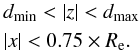 (1)The parameter d is in units of be for Method 1, Re for Method 2, and kpc for Method 3. For each minor axis bin, we consider fibers both above and below the disk. We use the xpos and ypos fits extensions in the RSS file at the wavelength of 5000 Å to determine the location of each fiber. The position of the fiber can shift as a function of wavelength due to differential atmospheric refraction (DAR). Since each galaxy can have a different size, shape and IFU bundle size, the number of fibers that are located in a given minor axis bin varies from galaxy to galaxy. However, we have selected our sample so that every galaxy contributes some fibers to each bin.
The spectra from each fiber were first corrected using the masks and error information provided in the RSS files. Any wavelength pixel that was flagged to be masked was considered as a bad pixel and the flux was interpolated over it. If a given fiber had less than 100 good pixels, the fiber was removed from the stack, which occurred in ≲0.5% of the fibers. The wavelength regions dominated by sky line residuals were also removed and interpolated over. Since we are considering the spectral range from 3600 to 7000 Å, there are only three dominant sky lines at 5578.5, 5894.6, and 6301.7 Å. The flux from each spectrum was converted into surface brightness using the redshift for each galaxy.
Before stacking, the spectra were also corrected for galactic rotation. Since most of the individual spectra have very low S/N, we could not measure directly the velocity shift from the emission lines. Instead, we derive the rotation curve from the Hα emission line measured along the major axis (Moran et al. 2010). We fit a cubic function to Vc(R), where R is the distance along the major axis and we assume that the rotation curve does not vary as a function distance from the galactic midplane. This velocity rotation correction made only a slight difference to our measurements of the widths of the stacked emission lines. As noted in Sect. 3, some of the broadening of the emission lines seen in the outer minor axis bins may be attributed to inaccuracies in this procedure and the assumption that the velocity is constant with distance along the minor axis.
Once all the spectra for the different bins were corrected, shifted to rest frame and put on the same wavelength grid, they were stacked by the following procedure. At each wavelength pixel, we took the mean surface brightness of all the fibers excluding the lowest and highest 10% (e.g., D’Souza et al. 2014), with the errors for each spectrum propagated appropriately to a stacked error. We chose a clipped mean instead of a weighted mean to better exclude outliers and be less biased by extreme regions (like an off axis H ii region or an unseen satellite) or fibers with extreme negative or positive values. Since we are interested in DIG in the outskirts and this should be a relatively low surface brightness, diffuse feature, taking a clipped mean over just taking a mean was less biased and closer to the median averaged stacked spectrum, with a difference between the clipped mean and median of ≲10%. We chose the clipped mean over a median to have a better handle on propagating the errors to have a stacked error spectrum as well as the stacked surface brightness spectrum. Regardless of whether we took the median, mean, or clipped mean, the general results and trends were the same, only the value of the surface brightnesses changed. We did not perform any additional sigma clipping because most of the spectra had very low S/N, usually ≲0.5 and so this would greatly limit the number of fibers to stack.
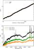 |
Fig. 3 Top: S/N in the blue (4000–5500 Å) as a function of the number of fibers stacked. The S/N scales close to the theoretical expectation of N0.5 overplotted in orange. This demonstrates that we are not currently limited by the background or systematics in this wavelength range. Bottom: S/N for three different be bins as a function of wavelength for the full sample. The S/N is higher for the emission lines. There is a dip ~5700Å around where the two spectrographs are joined and an increase in background noise from high pressure sodium streetlamps. |
In Fig. 3, the top panel shows that the S/N in the blue part of the spectrum (4000–5500 Å) increases roughly as the square root of the number of fibers stacked, showing that we are not limited by residual sky background subtraction errors in this wavelength range. The example shown in this figure is from the 3.0–3.5 be bin of the full stack of 49 galaxies using Method 1. The other minor axis bins and methods give similar results. We note that for the first few hundred fibers, the trend is not as smooth because each fiber was chosen randomly and each galaxy has a different surface brightness profile and therefore different average S/N. The bottom panel of Fig. 3 shows the S/N as a function of wavelength (in rest frame) for the stacked spectrum in three different minor axis bins. There is a dip in the S/N around 5700Å which could be from where the two spectrographs are joined, between 5900–6300Å in observer wavelength frame, and/or by high pressure sodium from streetlamps which is a broad feature around 5900Å in the observers frame causing an increase in the background noise. The S/N also decreases shortwards of 4500Å where the throughput of the spectrographs is lower. As expected, the average S/N shows spikes where there are strong emission lines.
The total number of galaxies, number of fibers, surface brightness estimate of the continuum in the blue, S/N in the blue, and the S/N near Hα for the outer minor axis bins are provided in Table 1 for each stack with be> 2, and z > 4kpc for the large-z sample. We provide results from Method 3 for the large-z sample instead of Method 1. For the full sample with 49 galaxies, the number of fibers stacked ranges from 2981 in the inner bins to 2281 in the outermost bins and for the large-z sample it ranges between 331 and 1871 fibers. The outermost bins for the large-z sample are larger because more fibers are needed in order to increase the S/N to a high enough level to be able to detect emission lines. The continuum S/N in the blue drops from 40 in the disk to approximately five in the outer regions, while the S/N of Hα drops from 72 to eight for the samples with only 24 galaxies. The S/N of the emission lines are always about twice that of the continuum. For the large-z bins the S/N in the continuum can be below one and for Hα the S/N is around four. This demonstrates the need for stacking many galaxies to detect the eDIG at >5 kpc (or >1.5Re) from the galactic plane. An example of a stacked spectrum between 2.5 and 3.0 be is shown in Fig. 4. The 1 and 3σ error contours are also plotted. As can be seen the main strong emission lines Hα, Hβ, [O ii]λλ3726, 3729, [O iii]λ5007, [N ii]λλ6549, 6584, and [S ii]λλ6717, 6731 are easily detected at greater than 3σ confidence. A small bump in the spectrum is visible near the region where the two spectrographs are joined.
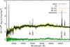 |
Fig. 4 Example of the spectrum (in rest frame) obtained by stacking fibers from the full sample between 2.5 and 3.0 be (black solid). The 1 and 3σ errors on the continuum are shown in the orange and yellow bands. The best-fit model spectrum (blue dotted) is overplotted along with the residuals from the fit (green). The bright emission lines Hα, Hβ, [O ii], [O iii], [N ii], and [S ii], discussed in this paper, are labeled. |
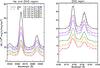 |
Fig. 5 Enlargement of the emission lines for the full sample for various be bins using Method 1. The data is shown as the solid line and the emission line fits are the dashed lines, with the different colors corresponding to different be bins. The spectra have been scaled in the vertical direction for clarity, with the amount shown in the legend. |
2.3. Spectral fitting
For finding the emission line surface brightnesses, we used a version of the MPA-JHU spectral fitting code (Tremonti et al. 2004) that has been modified by C. Tremonti for the MaNGA spectra. The MPA-JHU spectral fitting method uses the models from Bruzual & Charlot (2003), with three metalicities and 11 different ages to fit the stellar continuum with the emission lines masked, and then fits the emission lines as Gaussians. Line surface brightnesses and widths with errors are output by the code. We note that the subsolar metalicity models consistently had a lower χ2; this is not unexpected since almost all the galaxies in our sample have stellar masses less than 1010 M⊙, below the “knee” in the stellar mass-metallicity relation.
As shown in Fig. 4 with the blue dotted line, the best-fit model spectrum agrees well with the data (the residuals (data-fit) shown in green in the plot are always near zero). Figure 5 presents a closer look at some of the main emission lines. We plot the wavelength regions around Hα and [N ii], as well as around [S ii], for the minor axis bins from 0 to 4 be. Even though the S/N decreases significantly in the outermost bins, the emission lines are well fit by simple Gaussians and the emission lines are clearly detected.
Minor axis bin properties.
3. Results
We present our results of the surface brightnesses of the bright optical emission lines from the stacked spectra. First, we discuss the results from the full sample of 49 galaxies in Sect. 3.1. For the full sample, the minor axis bins for all three methods are given in Table C.1. We have bins for the central areas of the galaxies within the main disk to aid in understanding how the halo gas differs from interstellar medium gas. We checked the central bins for AGN contamination by stacking from 0.0–0.2 and 0.2–1.0 be, and there was no noticeable difference in the line ratios. In 0.0–0.2 be stacks, we found three galaxies that are consistent with having an AGN. To extend farther into the halo, the large-z sample contains 16 galaxies that have fibers out to at least 9kpc and we discuss these results in Sect. 3.2. The minor axis bins are the same as the full sample with additional bins for Method 2 between 1.0–1.2, 1.2–1.4, 1.4–1.7, 1.6–1.9, and 1.7–2.0Re, and for Method 3 between 4.0–4.5, 4.5–5.0, 5.0–6.0, 6.0–7.0, 7.0–9.0, and 7.0–10.0kpc. We do not include the analysis performed with Method 1 for the large-z stack, but the results from Method 1 are similar to Method 2 for the large-z sample. Then in Sect. 3.3 we present subsamples, where we split the full sample into two halves, by sSFR (at 5.8 × 10⁻¹⁰ yr-1), by concentration index (at 2.44), and by stellar mass (at 3.73 × 10⁹M⊙) with the same minor axis bins as the full sample. As shown in Table 1, the S/N in the Hα region ≳3 in all bins with detections. For the large-z sample, many of the other emission lines are no longer detected in the outer bins, however [O ii] and Hα can still be detected in most of them. A full discussion of the detection limits is given in Sect. 3.2. Table C.1 gives the surface brightness values for the bright emission lines at each minor axis bin for the three stacking methods for the full sample and subsamples split by various galactic properties.
3.1. Full sample
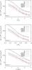 |
Fig. 6 Surface brightness profiles of the six brightest emission lines (different colors) as a function of distance from the midplane for the full sample with the three different stacking methods. The errors are from the spectral fitting. Top panel is with Method 1, middle with Method 2, and the bottom is with Method 3, see Sect. 2.2 for details of these methods. |
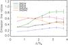 |
Fig. 7 Ratios of the bright emission lines for the full sample using Method 1 as a function of z. |
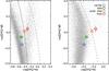 |
Fig. 8 BPT diagram of the different galactic regions from the full sample with the K03 (solid) and K01 (dashed) demarcation lines. The central, disk, outer disk, and halo regions correspond to the 0.0–1.0, 1.0−1.5, 2.0–2.5, 3.0–3.5 be bins, respectively. The error bars correspond to the errors from the spectral fitting, propagated appropriately. Emission line ratios measured from SDSS DR7 fiber spectra for the main galaxy sample are plotted as gray dots. |
The surface brightness profiles of the bright emission lines, Hα, Hβ, [O ii]λ3729, [O iii]λ5007, [N ii]λ6584, and [S ii]λ6731, as a function of distance along the minor axis for the full sample of 49 late-type galaxies are shown for the three stacking methods in Fig. 6. The three methods give similar profiles and all have clear detections of the six emission lines, which exponentially decrease with distance. Hα is the dominant emission line near the disk, but [O ii]λ3729 is nearly as strong as Hα at distances greater than ~3be. [S ii]λ6731 is the weakest. The errors shown in the plot in color are the ones provided by the emission line spectral fitting code. In general there is not a huge difference amongst the different stacking methods. However, Method 1 seems to have breaks in the emission line profiles whereas Method 3 is smoother and more shallow. This is probably because we are stacking across galaxies with a range of sizes leading to a smoothing of the profiles in Method 3. The relative strengths of the emission lines do not vary significantly for the different methods. All of the emission line surface brightnesses are provided in Table C.1.
In Fig. 7 we show the radial dependence of ratios of some of the bright emission lines, for simplicity only for Method 1 (z/be). [O iii]λ5007/[O ii]λ3729 decreases with increasing distance from the mid-plane, which is expected as the gas is farther away from the main ionization source (OB stars in the disk). [O ii]λ3729/Hα shows a strong increase with distance. This could be indicative of gas temperatures increasing at large distances from the disk (e.g., Haffner et al. 2009). In the outermost bin it almost approaches unity. The ratios [N ii]λ6584/Hα, [S ii]λ6731/Hα increase by about 50% between the inner- and outermost bins, whereas the ratio of [S ii]λ6731/[N ii]λ6584 remains roughly constant with height. Here [S ii]λ6731/Hα varies from 0.2 in the center to 0.3 in the outskirts and [N ii]λ6584/Hα from 0.4 to 0.5. These results agree with previous studies of the DIG in the MW and other galaxies (e.g., Haffner et al. 2009; Zhang et al. 2016), who found that the ratios [N ii]/Hα and [S ii]/Hα in DIG are usually enhanced compared to classic H ii regions.
To gain further insight, in Fig. 8 we have also examined correlations between different line ratios in a series of “BPT” diagrams similar to those introduced by Baldwin et al. (1981) to distinguish between gas that is being photo-ionized by young stars in H ii regions, and gas that is being photo-ionized by the central source in an active galactic nucleus (AGN). For all the BPT diagrams [S ii] refers to the sum of two [S ii]λλ6717, 6731 emission lines. For clarity, we have only plotted about half the be bins, sampling different regions of the galaxy. The chosen bins are 0.0–1.0 be for the center of the galaxy, 1.0–1.5 be for the disk, 2.0–2.5 be as the outer disk, and 3.0–3.5 be for the region outside the disk (which we term the halo) with errors from the spectral fitting code. For reference, emission line ratios from galaxies from the SDSS DR7 main spectroscopic sample are plotted in the background as gray small dots. These emission line ratios are obtained from three arcsecond diameter single fiber spectra that typically sample light from the inner 1–3 kpc of the galaxy, meaning that these ratios often pertain to emission line gas present in galactic bulges rather than disks. As a consequence, many emission line ratios characteristic of ionization from an AGN are found.
The empirical demarcation curve separating star-forming galaxies and AGN from Kauffmann et al. (2003, K03) and the theoretical curve proposed by Kewley et al. (2001, K01) are plotted as solid and dashed lines, respectively. As can be seen, the emission line ratios for the central stack lie in the region of the diagram appropriate for photo-ionization from young stars. As we move away from the center, there is a clear trend with distance z for the emission line ratios to move into the so-called “composite” region of the diagram. As discussed in K03, emission line gas sampled by the single fiber SDSS spectra likely lie in this region of the diagram because photo-ionization is from a mixture of young stars and a central AGN. By comparing emission line ratios from similar galaxies at different redshifts in the SDSS main sample, K03 demonstrated that the average emission line ratios shifted systematically from the AGN to the star-forming sections of the BPT diagrams as distance (redshift) increased and the physical aperture spanned by the SDSS fiber became larger. In this study, we are sampling regions of the galaxy very far away from any central supermassive black hole, so the physical explanation must be different. As discussed in K01, gas which is heated by shocks is also expected to produce emission lines with ratios lying in the “composite” part of the diagram. Shock-heating of gas falling into dark matter halos is a fundamental physical process in galaxy formation and a proper accounting of such heating process is likely critical to the interpretation of our observations. Another phenomenon that should be considered when interpreting these diagrams is the effect of a diluted radiation field which would also cause a shift in the line ratios. We leave the full investigation of the differences and trends of the emission lines and ratios for a future paper.
3.2. Large-z sample
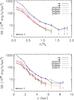 |
Fig. 9 Surface brightnesses of the bright emission lines for the large-z stack as a function of z for stacking methods 2 (top) and 3 (bottom). Upper limits are indicated by the arrows. |
With our stack of 16 galaxies extending past 9kpc, we can study emission line profiles out to larger distances from the disk. This sample was chosen so each galaxy simultaneously had fibers that extended out to at least 2Re and 9kpc so they would be part of both stacking Methods 2 and 3. We relaxed the constraint on b/a so each galaxy must have b/a< 0.4. This increased the sample by another four galaxies. Because the galaxies have a larger range of inclinations and we wanted to ensure that the detections in the outer bins for each galaxy were from the halo and not from the outer disk, we made an additional requirement on the size of be. Each galaxy must have be ≤ 2kpc, so at heights ≳5kpc (or about 1 Re) we are probing the halo. The galaxies that were included in this sample are marked in Table A.1 and the four additional galaxies with 0.3 < b/a < 0.4 are shown below the line. In Appendix D Figs. D.1–D.4, we have provided maps of the continuum and Hα emission for each galaxy in this sample.
In Fig. 9 we show the emission line surface brightness profiles for the large-z sample with stacking methods 2 and 3. We provide upper limits where the signal is not reliably detected. This is done by combining between 1000 and 1500 sky spectra into 30 independent stacks and adding in artificial emission lines of known flux with Gaussian profiles and widths the same as that observed in the stacked spectra with detections. We decreased the strength of the emission lines until the error on the line fluxes are greater than 20% of the true value. This determines the values of the upper limits plotted in Fig. 9 and any value that was less than this is considered to not be reliably detected. Due to the wavelength-dependence of the S/N (see Fig. 3) these limits are at slightly different levels for different lines. At large distances, [O ii] becomes comparable with Hα beyond 1.0 Re and 3kpc in the stack. Intriguingly, with both stacking methods all detectable lines in the halo, [O ii], Hα, and for Method 3 also [N ii], the line surface brightnesses appear to flatten at these large distances. This could indicate a change in the heating source at these distances. Future analysis with larger samples from the complete MaNGA survey will be useful for solidifying the analysis of line ratios at large distances from the disk.
3.3. Results split by sSFR, C, and Mstar
With a sample of 49 galaxies we can split the sample in half (2 × 24) and still have enough S/N for reliable detections of the bright emission lines (see Table 1). The amount of ionized gas and possible additional heating source(s) could depend on galactic properties. For example, the amount of eDIG present is known to depend on the star-formation rate of the galaxy (e.g., Rossa & Dettmar 2003a). We have, therefore, split the full sample in half according to sSFR (at 5.8 × 10⁻¹⁰ yr-1), C (at 2.44), and Mstar (at 3.7 × 10⁹M⊙). These quantities for the individual galaxies are provided in Table A.1. The surface brightnesses of the bright emission lines for these subsamples are also given in Table C.1.
Figure 10 is similar to Fig. 6 but only for Hα of the different subsamples for the three stacking methods. The full sample (black solid line) is also given for reference. It is clearly seen that the largest differences in Hα line surface brightness are between the high and low sSFR subsamples for Method 1 and 2, which is expected due to the relationship between eDIG and star-formation. All three stacking methods show very similar trends, except for Method 3 for the high sSFR subsample. For Methods 1 and 2 the high sSFR subsample has the highest Hα surface brightness at all distances, but for Method 3 this is only true at z ≲ 1kpc and then the high Mstar dominates. This is probably because the higher Mstar galaxies also have larger disks compared to the other subsamples, so at the same physical distance, the high Mstar sample is at a smaller Re compared to the other samples. Interestingly, the difference in line surface brightness for the sSFR subsamples is roughly the same at all distances with Methods 1 and 2. The favored interpretation for higher eDIG surface brightnesses is that galactic winds have driven out more gas in galaxies with stronger star-formation. Galactic winds generally occur as bi-conical outflows from the central region of the galaxy with opening angles of ~60 deg. With a larger sample, we will test for an azimuthal dependence on the Hα surface brightness. Figure 11 shows differences in emission line ratios for the high sSFR and low sSFR subsamples. As in Fig. 8, we have only plotted a fraction of the minor axis bins for clarity. The central, disk, outer disk, and halo regions again correspond to the 0.0–1.0, 1.0–1.5, 2.0–2.5, 3.0–3.5 be bins, respectively. As can be seen, the high sSFR data points are concentrated closer to the star-forming region of the BPT diagrams than the low sSFR data points. This is consistent with the hypothesis that a larger fraction of the ionizing photons responsible for exciting the gas arise from young stars in the actively star-forming systems. To ensure that these differences are significant and not due to a small sample size, we also split the full sample randomly in half six times and compared the emission line ratios for the halo bin, where the differences are the largest in the BPT diagram. The mean and standard deviation of the absolute value of the differences for the randomly split samples between log ([O iii] /Hβ), log ([N ii] /Hα), and log ([S ii] /Hα) are 0.04 ± 0.02, 0.09 ± 0.06, and 0.03 ± 0.02, respectively. The changes we see in the two sSFR populations are greater than this.
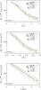 |
Fig. 10 Hα surface brightness profile as a function of z for various subsamples with the three different stacking methods, top panel is with Method 1, middle with Method 2, and the bottom is with Method 3. |
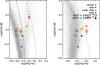 |
Fig. 11 Similar to Fig. 8 but showing the subsamples that were split by sSFR. The high sSFR galaxies are shown as open circles and the low sSFR galaxies as filled triangles with the colors corresponding to regions along the minor axis like in Fig. 8. |
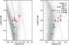 |
Fig. 12 As Fig. 11 but split by C, with high C galaxies as open circles and low C galaxies as filled triangles. |
When split by Mstar or C, differences in Hα surface brightness profiles are much smaller (typically less than a factor of 1.5) for Methods 1 and 2 (Fig. 10), but significant differences in emission line ratios between the sub-samples remain. When split by concentration, Fig. 12 shows that the low C points are more clustered toward the star-formation region. Interestingly, the outermost “halo point” for the low C sample regresses back to the star forming area, particularly in the diagram with [N ii]/Hα on the x-axis. In contrast, there is a 0.4 dex increase in log [N ii]/Hα from the inner disk to the outer halo for the high C sample. When split by Mstar, similar trends are seen – low mass galaxies cluster toward the star-forming region of the diagram, whereas high-mass galaxies are generally in the composite region, particularly at a large distance from the disk plane. The trend for [O iii]/Hβ, [N ii]/Hα, and [S ii]/Hα to increase as a function of distance from the disk is strongest for high Mstar galaxies. It is well established that dark matter halo mass scales most strongly with stellar mass, and thus the temperature of shock-heated, virialized halo gas could also scale most strongly with stellar mass. In future work we plan to investigate whether these trends can be caused by such scalings.
We have also plotted only the changes in the [N ii]/Hα ratio with distance for the different samples, shown in Fig. 14. There is no significant difference amongst the different stacking methods. [N ii]/Hα can be a temperature indicator, assuming the relative abundances of nitrogen and hydrogen are constant. This assumption might not be valid in the halo, where for resolved populations studies of very nearby galaxies a range of metalicity gradients is seen (Monachesi et al. 2016). For most of the subsamples this ratio slightly increases by 0.1 to 0.2 with distance, except for Mstar subsamples. The high Mstar sample increases from ~0.45 to 0.8 in Method 1 and 2 and to 0.6 in Method 3. The ratio in the low Mstar sample stays constant in all three methods. This is consistent with Fig. 13 where the low Mstar sample at all distances stays within the star-formation area of the BPT diagram.
For more details, Table C.1 lists the surface brightnesses of all the bright emission lines using the three stacking methods for each minor axis bin for all the samples (excluding the large-z sample).
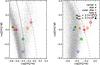 |
Fig. 13 As Fig. 11 but split by Mstar, with high Mstar galaxies as open circles and low Mstar galaxies as filled triangles. |
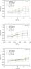 |
Fig. 14 Ratio of emission lines [N ii] and Hα as a function of z for various subsamples with the three different stacking methods, top panel is with Method 1, middle with Method 2, and the bottom is with Method 3. |
4. Conclusion
Studying eDIG around nearby galaxies is a challenging task due to its naturally low surface brightness. Previous spectroscopic studies usually observed individual, very nearby galaxies with long integration times to detect eDIG out to a few kpc. Using the MaNGA survey and with the technique of stacking spectra across several dozen galaxies, we can observe the eDIG into the halo and study the radial trends for an average galaxy population. We have stacked across the galaxies using three different methods for normalizing the distance from the midplane, by minor axis effective radii (be), major axis effective radii (Re), and physical distance (kpc). In most cases the three methods were in agreement.
In this current paper we have the following conclusions: First, we can clearly detect emission lines out to ~4kpc above the disk with our full sample of 49 galaxies (Figs. 5 and 6). The emission line ratios (Fig. 7) are consistent with what has previously been observed in individual nearby galaxies including the Milky Way. Second, with only 16 galaxies observed to larger radii, we can already have some detections for the bright emission lines, namely Hα and [O ii], and upper limits of the other bright emission lines out to ~9kpc. Past ~6kpc the [O ii] and Hα surface brightnesses are comparable and slightly flatten, suggesting a possible change in the heating source, such as HOLMES, shocks, inflows, etc (Fig. 9). Third, by splitting our sample by different galactic properties, we clearly detect changes to the eDIG in the outer disk and halo. The emission line surface brightnesses are higher both in the disk and halo for the high sSFR galaxies compared to the low sSFR galaxies (Fig. 10). The high Mstar sample has the highest [N ii]/Hα ratio with the strongest increase with distance, indicating a large temperature gradient. The high C galaxies also show a slight increase of [N ii]/Hα and the low sSFR sample increases as well (Fig. 14). Lastly, in the BPT diagrams, all the split subsamples occupy different areas of the diagram and show different trends with distance (Figs. 11–13). The low Mstar, low C, and high sSFR tend to lie near the starforming region of the BPT diagram. The other subsamples’ outer disk and halo values are between the K03 and K01 lines in the [N ii]/Hα diagram, and past K01 in the [S ii]/Hα diagram. This shows that eDIG properties depend on galactic properties: sSFR, bulge to disk ratio, and stellar mass.
As the MaNGA observations continue, the sample size will keep increasing, allowing for further study of outskirts of galaxies and eDIG. By the end of the MaNGA survey, with ~300 galaxies out to 4kpc and ~100 galaxies out to 9kpc, we can better determine the dependence of the eDIG on galactic properties. In combination with models we can improve our understanding of the possible additional heating source(s) and the extent of the eDIG.
Acknowledgments
Funding for the Sloan Digital Sky Survey IV has been provided by the Alfred P. Sloan Foundation, the US Department of Energy Office of Science, and the Participating Institutions. SDSS-IV acknowledges support and resources from the Center for High-Performance Computing at the University of Utah. The SDSS web site is www.sdss.org. SDSS-IV is managed by the Astrophysical Research Consortium for the Participating Institutions of the SDSS Collaboration including the Brazilian Participation Group, the Carnegie Institution for Science, Carnegie Mellon University, the Chilean Participation Group, the French Participation Group, Harvard-Smithsonian Center for Astrophysics, Instituto de Astrofísica de Canarias, The Johns Hopkins University, Kavli Institute for the Physics and Mathematics of the Universe (IPMU)/University of Tokyo, Lawrence Berkeley National Laboratory, Leibniz Institut für Astrophysik Potsdam (AIP), Max-Planck-Institut für Astronomie (MPIA Heidelberg), Max-Planck-Institut für Astrophysik (MPA Garching), Max-Planck-Institut für Extraterrestrische Physik (MPE), National Astronomical Observatory of China, New Mexico State University, New York University, University of Notre Dame, Observatário Nacional/MCTI, The Ohio State University, Pennsylvania State University, Shanghai Astronomical Observatory, United Kingdom Participation Group, Universidad Nacional Autónoma de México, University of Arizona, University of Colorado Boulder, University of Oxford, University of Portsmouth, University of Utah, University of Virginia, University of Washington, University of Wisconsin, Vanderbilt University, and Yale University. D.B. acknowledges support from grant RSF 14-50-00043. M.A.B. acknowledges NSF-AST/1517006.
References
- Baldwin, J. A., Phillips, M. M., & Terlevich, R. 1981, PASP, 93, 5 [NASA ADS] [CrossRef] [EDP Sciences] [Google Scholar]
- Barnes, J. E., Wood, K., Hill, A. S., & Haffner, L. M. 2014, MNRAS, 440, 3027 [NASA ADS] [CrossRef] [Google Scholar]
- Binette, L., Drissen, L., Ubeda, L., et al. 2009, A&A, 500, 817 [NASA ADS] [CrossRef] [EDP Sciences] [Google Scholar]
- Blanton, M. R., Bershady, M. A., Abolfathi, B., et al. 2017, AJ, submitted [arXiv:1703.00052] [Google Scholar]
- Bruzual, G., & Charlot, S. 2003, MNRAS, 344, 1000 [NASA ADS] [CrossRef] [Google Scholar]
- Bryant, J. J., Owers, M. S., Robotham, A. S. G., et al. 2015, MNRAS, 447, 2857 [NASA ADS] [CrossRef] [Google Scholar]
- Bundy, K., Bershady, M. A., Law, D. R., et al. 2015, ApJ, 798, 7 [NASA ADS] [CrossRef] [Google Scholar]
- Calzetti, D. 2001, PASP, 113, 1449 [NASA ADS] [CrossRef] [Google Scholar]
- Collins, J. A., & Rand, R. J. 2001, in Gas and Galaxy Evolution, eds. J. E. Hibbard, M. Rupen, & J. H. van Gorkom, ASP Conf. Ser., 240, 392 [Google Scholar]
- Collins, J. A., Benjamin, R. A., & Rand, R. J. 2002, ApJ, 578, 98 [NASA ADS] [CrossRef] [Google Scholar]
- Dettmar, R.-J. 1990, A&A, 232, L15 [Google Scholar]
- Drory, N., MacDonald, N., Bershady, M. A., et al. 2015, AJ, 149, 77 [NASA ADS] [CrossRef] [Google Scholar]
- D’Souza, R., Kauffman, G., Wang, J., & Vegetti, S. 2014, MNRAS, 443, 1433 [NASA ADS] [CrossRef] [Google Scholar]
- Finkbeiner, D. P. 2003, ApJS, 146, 407 [NASA ADS] [CrossRef] [Google Scholar]
- Flores-Fajardo, N., Morisset, C., Stasińska, G., & Binette, L. 2011, MNRAS, 415, 2182 [NASA ADS] [CrossRef] [Google Scholar]
- Greenawalt, B., Walterbos, R. A. M., & Braun, R. 1997, ApJ, 483, 666 [NASA ADS] [CrossRef] [Google Scholar]
- Greene, J. E., Janish, R., Ma, C.-P., et al. 2015, ApJ, 807, 11 [NASA ADS] [CrossRef] [Google Scholar]
- Gunn, J. E., Siegmund, W. A., Mannery, E. J., et al. 2006, AJ, 131, 2332 [NASA ADS] [CrossRef] [Google Scholar]
- Haffner, L. M., Dettmar, R.-J., Beckman, J. E., et al. 2009, Rev. Mod. Phys., 81, 969 [NASA ADS] [CrossRef] [Google Scholar]
- Heald, G. H., Rand, R. J., Benjamin, R. A., & Bershady, M. A. 2006a, ApJ, 647, 1018 [NASA ADS] [CrossRef] [Google Scholar]
- Heald, G. H., Rand, R. J., Benjamin, R. A., Collins, J. A., & Bland-Hawthorn, J. 2006b, ApJ, 636, 181 [NASA ADS] [CrossRef] [Google Scholar]
- Heald, G. H., Rand, R. J., Benjamin, R. A., & Bershady, M. A. 2007, ApJ, 663, 933 [NASA ADS] [CrossRef] [Google Scholar]
- Hidalgo-Gámez, A. M. 2006, AJ, 131, 2078 [NASA ADS] [CrossRef] [Google Scholar]
- Ho, I.-T., Medling, A. M., Bland-Hawthorn, J., et al. 2016, MNRAS, 457, 1257 [NASA ADS] [CrossRef] [Google Scholar]
- Hoopes, C. G., & Walterbos, R. A. M. 2003, ApJ, 586, 902 [NASA ADS] [CrossRef] [Google Scholar]
- Hoopes, C. G., Walterbos, R. A. M., & Rand, R. J. 1999, ApJ, 522, 669 [NASA ADS] [CrossRef] [Google Scholar]
- Hubble, E. P. 1926, ApJ, 64, 321 [NASA ADS] [CrossRef] [Google Scholar]
- Kamphuis, P., Peletier, R. F., Dettmar, R.-J., et al. 2007, A&A, 468, 951 [NASA ADS] [CrossRef] [EDP Sciences] [Google Scholar]
- Kauffmann, G., Heckman, T. M., Tremonti, C., et al. 2003, MNRAS, 346, 1055 [Google Scholar]
- Kennicutt, Jr., R. C. 1998, ARA&A, 36, 189 [Google Scholar]
- Kewley, L. J., Dopita, M. A., Sutherland, R. S., Heisler, C. A., & Trevena, J. 2001, ApJ, 556, 121 [Google Scholar]
- Law, D. R., Yan, R., Bershady, M. A., et al. 2015, AJ, 150, 19 [NASA ADS] [CrossRef] [Google Scholar]
- Lehnert, M. D., & Heckman, T. M. 1994, ApJ, 426, L27 [NASA ADS] [CrossRef] [Google Scholar]
- Madsen, G. J., Reynolds, R. J., & Haffner, L. M. 2006, ApJ, 652, 401 [NASA ADS] [CrossRef] [Google Scholar]
- Monachesi, A., Bell, E. F., Radburn-Smith, D. J., et al. 2016, MNRAS, 457, 1419 [NASA ADS] [CrossRef] [Google Scholar]
- Moran, S. M., Kauffmann, G., Heckman, T. M., et al. 2010, ApJ, 720, 1126 [NASA ADS] [CrossRef] [Google Scholar]
- Otte, B., Reynolds, R. J., Gallagher, III, J. S., & Ferguson, A. M. N. 2001, ApJ, 560, 207 [NASA ADS] [CrossRef] [Google Scholar]
- Putman, M. E., Peek, J. E. G., & Joung, M. R. 2012, ARA&A, 50, 491 [NASA ADS] [CrossRef] [Google Scholar]
- Rand, R. J. 1996, ApJ, 462, 712 [CrossRef] [Google Scholar]
- Rand, R. J. 1997, ApJ, 474, 129 [NASA ADS] [CrossRef] [Google Scholar]
- Rand, R. J. 2000, ApJ, 537, L13 [NASA ADS] [CrossRef] [Google Scholar]
- Rand, R. J., Kulkarni, S. R., & Hester, J. J. 1990, ApJ, 352, L1 [NASA ADS] [CrossRef] [Google Scholar]
- Reynolds, R. J. 1971, Ph.D. Thesis, The University of Wisconsin – Madison [Google Scholar]
- Reynolds, R. J. 1990, in The Galactic and Extragalactic Background Radiation, eds. S. Bowyer, & C. Leinert, IAU Symp., 139, 157 [Google Scholar]
- Reynolds, R. J. 1991, in The Interstellar Disk-Halo Connection in Galaxies, ed. H. Bloemen, IAU Symp., 144, 67 [Google Scholar]
- Reynolds, R. J., & Cox, D. P. 1992, ApJ, 400, L33 [NASA ADS] [CrossRef] [Google Scholar]
- Reynolds, R. J., Scherb, F., & Roesler, F. L. 1973, ApJ, 185, 869 [NASA ADS] [CrossRef] [Google Scholar]
- Reynolds, R. J., Haffner, L. M., & Tufte, S. L. 1999, ApJ, 525, L21 [Google Scholar]
- Rossa, J., & Dettmar, R.-J. 2003a, A&A, 406, 493 [NASA ADS] [CrossRef] [EDP Sciences] [Google Scholar]
- Rossa, J., & Dettmar, R.-J. 2003b, A&A, 406, 505 [NASA ADS] [CrossRef] [EDP Sciences] [Google Scholar]
- Sánchez, S. F., Kennicutt, R. C., Gil de Paz, A., et al. 2012, A&A, 538, A8 [NASA ADS] [CrossRef] [EDP Sciences] [Google Scholar]
- Shimasaku, K., Fukugita, M., Doi, M., et al. 2001, AJ, 122, 1238 [NASA ADS] [CrossRef] [Google Scholar]
- Smee, S. A., Gunn, J. E., Uomoto, A., et al. 2013, AJ, 146, 32 [Google Scholar]
- Tremonti, C. A., Heckman, T. M., Kauffmann, G., et al. 2004, ApJ, 613, 898 [NASA ADS] [CrossRef] [Google Scholar]
- White, S. D. M., & Rees, M. J. 1978, MNRAS, 183, 341 [NASA ADS] [CrossRef] [Google Scholar]
- Wood, K., Hill, A. S., Joung, M. R., et al. 2010, ApJ, 721, 1397 [NASA ADS] [CrossRef] [Google Scholar]
- Yan, R., Tremonti, C., Bershady, M. A., et al. 2016a, AJ, 151, 8 [NASA ADS] [CrossRef] [Google Scholar]
- Yan, R., Bundy, K., Law, D. R., et al. 2016b, AJ, 152, 197 [NASA ADS] [CrossRef] [Google Scholar]
- Zurita, A., Rozas, M., & Beckman, J. E. 2000, A&A, 363, 9 [NASA ADS] [Google Scholar]
- Zurita, A., Beckman, J. E., Rozas, M., & Ryder, S. 2002, A&A, 386, 801 [NASA ADS] [CrossRef] [EDP Sciences] [Google Scholar]
Appendix A: Additionnal table
Galaxy properties.
Appendix B: Inclination effect
The restriction on inclination for this analysis is that each galaxy must have a b/a< 0.3. Thus, many galaxies in our sample are not truly edge-on (see Fig. 1 and Table A.1). When binning vertically above and below the galaxy midplane we are most likely stacking different areas from the each galaxy in the sample. In other words for a highly inclined galaxy, 2 kpc above the midplane may already be in the halo, but for a less inclined galaxy would still be in the outer disk. To see how this mixing affects our results, we have stacked galaxies with b/a ≤ 0.2 and compared them with the full sample (which has b/a< 0.3). We chose b/a = 0.2 as the cutoff because this is typically considered to be the intrinsic thickness of a galaxy when converting between b/a and inclination (Hubble 1926). Therefore, galaxies with b/a ≤ 0.2 should be edge-on systems. There are only 18 galaxies in this sample, which is why we can only do this comparison for with the full sample and not the split subsamples or large-z sample where the S/N would be too low in the outskirts. The full and near edge-on samples have similar median sSFR, C, and Mstar, so the differences seen between then are from different cuts in b/a. We have plotted this comparison on the BPT diagrams for the three stacking methods in Fig. B.1. We define center, disk, outer disk and halo for Method 1 as 0.0–1.0, 1.0–1.5, 2.0–2.5, and 3.0–3.5be, Method 2 as 0.0–0.2, 0.2–0.4, 0.4–0.6, and 0.8–1.0Re, and for Method 3 as 0.0–1.0, 1.0–1.5, 2.0–2.5, and 3.0–3.5kpc, respectively. Qualitatively the trend with distance from the midplane of the stacks’ emission line ratios to increase with distance and move away from the star forming region of the BPT diagrams is similar between the two samples. The main difference is an offset to lower [O iii]/Hβ for the full sample (filled triangles) compared to the near edge-on sample (open circles). The amount of this offset changes for each of the stacking methods. Method 1 in the outskirts has less of an offset compared to the other two methods, which is why for the full and split samples we show the BPT diagrams for Method 1. For this analysis, since the qualitative trends are same, our conclusions on the properties of eDIG in MaNGA galaxies are robust to the presence of galaxies that are not truly edge-on.
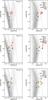 |
Fig. B.1 BPT diagrams comparing the ratios from the full sample (filled triangles) with galaxies in the sample that have a b/a ≤ 0.2 (open circles). top panel is with Method 1, middle with Method 2, and the bottom is with Method 3. |
Appendix C: Emission line surface brightnesses
We provide a table with the emission line surface brightness values for each bin and for the three stacking methods of the full sample and the split subsamples (Table C.1). The values are for the emission lines [O ii]λ3729, Hβ, [O iii]λ5007, Hα, [N ii]λ6584, [S ii]λ6717, and [S ii]λ6731 in units of 1036ergs-1kpc-2. The errors are from the spectral fitting.
Emission line surface brightnesses.
Appendix D: Continuum and Hα maps of large-z sample
In Figs. D.1–D.4, we show continuum and Hα maps for the 16 galaxies in the large-z sample, with a 1kpc scale bar. We also provide the SDSS image, like the ones shown in Fig. 1, with the MaNGA IFU footprint preceding the maps for each galaxy for reference. None of the galaxies show signs of merger activity or have bright extended emission in the outskirts that could affect our conclusions. Individually it is difficult to detect continuum or Hα emission in the outskirts (past 5kpc), but by stacking these galaxies we can detect Hα emission out to ~9kpc.
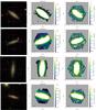 |
Fig. D.1 SDSS images, continuum maps and Hα maps for four of 16 galaxies (7962–12705, 8137–12701, 8137–12705, 8138–6103) in the large-z sample. See Figs. D.2–D.4 for the other 12 galaxies. |
All Tables
All Figures
|
Fig. 1 SDSS images of all the galaxies used in the analysis. The images are in the same order as Table A.1 (left to right, then top to bottom). Each box is 60 × 60 arcsec with the centers corresponding to the coordinates given in Table A.1. The four additional galaxies for the large-z sample are also included as the last four galaxies. |
| In the text | |
|
Fig. 2 Histograms showing the distributions of the MaNGA first year sample (black) and our sample of galaxies (orange) for various galactic properties. Panel a) shows the distribution of concentration index C with the vertical dashed purple line showing the division between late-type and early-type galaxies at C = 2.6. Panel b) gives the Mstar for the full sample (black), late-type galaxies (blue) defined by C < 2.6, and our sample (orange). Panel c) shows the inclination distribution (given by b/a) for the same sets of galaxies with the vertical dashed line at our cutoff b/a = 0.3. Panel d) shows the distribution of g-r colors. |
| In the text | |
|
Fig. 3 Top: S/N in the blue (4000–5500 Å) as a function of the number of fibers stacked. The S/N scales close to the theoretical expectation of N0.5 overplotted in orange. This demonstrates that we are not currently limited by the background or systematics in this wavelength range. Bottom: S/N for three different be bins as a function of wavelength for the full sample. The S/N is higher for the emission lines. There is a dip ~5700Å around where the two spectrographs are joined and an increase in background noise from high pressure sodium streetlamps. |
| In the text | |
|
Fig. 4 Example of the spectrum (in rest frame) obtained by stacking fibers from the full sample between 2.5 and 3.0 be (black solid). The 1 and 3σ errors on the continuum are shown in the orange and yellow bands. The best-fit model spectrum (blue dotted) is overplotted along with the residuals from the fit (green). The bright emission lines Hα, Hβ, [O ii], [O iii], [N ii], and [S ii], discussed in this paper, are labeled. |
| In the text | |
|
Fig. 5 Enlargement of the emission lines for the full sample for various be bins using Method 1. The data is shown as the solid line and the emission line fits are the dashed lines, with the different colors corresponding to different be bins. The spectra have been scaled in the vertical direction for clarity, with the amount shown in the legend. |
| In the text | |
|
Fig. 6 Surface brightness profiles of the six brightest emission lines (different colors) as a function of distance from the midplane for the full sample with the three different stacking methods. The errors are from the spectral fitting. Top panel is with Method 1, middle with Method 2, and the bottom is with Method 3, see Sect. 2.2 for details of these methods. |
| In the text | |
|
Fig. 7 Ratios of the bright emission lines for the full sample using Method 1 as a function of z. |
| In the text | |
|
Fig. 8 BPT diagram of the different galactic regions from the full sample with the K03 (solid) and K01 (dashed) demarcation lines. The central, disk, outer disk, and halo regions correspond to the 0.0–1.0, 1.0−1.5, 2.0–2.5, 3.0–3.5 be bins, respectively. The error bars correspond to the errors from the spectral fitting, propagated appropriately. Emission line ratios measured from SDSS DR7 fiber spectra for the main galaxy sample are plotted as gray dots. |
| In the text | |
|
Fig. 9 Surface brightnesses of the bright emission lines for the large-z stack as a function of z for stacking methods 2 (top) and 3 (bottom). Upper limits are indicated by the arrows. |
| In the text | |
|
Fig. 10 Hα surface brightness profile as a function of z for various subsamples with the three different stacking methods, top panel is with Method 1, middle with Method 2, and the bottom is with Method 3. |
| In the text | |
|
Fig. 11 Similar to Fig. 8 but showing the subsamples that were split by sSFR. The high sSFR galaxies are shown as open circles and the low sSFR galaxies as filled triangles with the colors corresponding to regions along the minor axis like in Fig. 8. |
| In the text | |
|
Fig. 12 As Fig. 11 but split by C, with high C galaxies as open circles and low C galaxies as filled triangles. |
| In the text | |
|
Fig. 13 As Fig. 11 but split by Mstar, with high Mstar galaxies as open circles and low Mstar galaxies as filled triangles. |
| In the text | |
|
Fig. 14 Ratio of emission lines [N ii] and Hα as a function of z for various subsamples with the three different stacking methods, top panel is with Method 1, middle with Method 2, and the bottom is with Method 3. |
| In the text | |
|
Fig. B.1 BPT diagrams comparing the ratios from the full sample (filled triangles) with galaxies in the sample that have a b/a ≤ 0.2 (open circles). top panel is with Method 1, middle with Method 2, and the bottom is with Method 3. |
| In the text | |
|
Fig. D.1 SDSS images, continuum maps and Hα maps for four of 16 galaxies (7962–12705, 8137–12701, 8137–12705, 8138–6103) in the large-z sample. See Figs. D.2–D.4 for the other 12 galaxies. |
| In the text | |
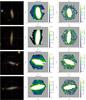 |
Fig. D.2 As Fig. D.1 for 8140–12702, 8247–12705, 8249–12701, and 8254–12702. |
| In the text | |
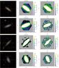 |
Fig. D.3 As Fig. D.1 for 8317–6101, 8329–12703, 8466–12703, and 8483–9102. |
| In the text | |
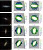 |
Fig. D.4 As Fig. D.1 for 8552–12702, 8552–6102, 8606–6101, and 8618–9102. |
| In the text | |
Current usage metrics show cumulative count of Article Views (full-text article views including HTML views, PDF and ePub downloads, according to the available data) and Abstracts Views on Vision4Press platform.
Data correspond to usage on the plateform after 2015. The current usage metrics is available 48-96 hours after online publication and is updated daily on week days.
Initial download of the metrics may take a while.