| Issue |
A&A
Volume 615, July 2018
|
|
|---|---|---|
| Article Number | A86 | |
| Number of page(s) | 10 | |
| Section | Planets and planetary systems | |
| DOI | https://doi.org/10.1051/0004-6361/201527071 | |
| Published online | 18 July 2018 | |
Thermal emission of WASP-48b in the Ks-band★
1
Astrophysics Group, Keele University,
Staffordshire
ST5 5BG,
UK
e-mail: b.j.clark@keele.ac.uk
2
Institute of Astronomy, University of Cambridge,
Madingley Road,
Cambridge
CB3 0HA,
UK
3
N. Copernicus Astronomical Centre, Polish Academy of Sciences,
Bartycka 18,
00-716
Warsaw,
Poland
4
Institute of Planetary Research, German Aerospace Center,
Rutherfordstrasse 2,
12489
Berlin,
Germany
5
SUPA, School of Physics and Astronomy, University of St. Andrews, North Haugh, Fife KY16 9SS, UK
Received:
28
July
2015
Accepted:
22
March
2018
We report a detection of thermal emission from the hot Jupiter WASP-48b in the Ks-band. We used the Wide-field Infra-red Camera on the 3.6-m Canada-France Hawaii Telescope to observe an occultation of the planet by its host star. From the resulting occultation lightcurve we find a planet-to-star contrast ratio in the Ks-band of 0.136 ± 0.014%, in agreement with the value of 0.109 ± 0.027% previously determined. We fit the two Ks-band occultation lightcurves simultaneously with occultation lightcurves in the H-band and the Spitzer 3.6- and 4.5-μm bandpasses, radial velocity data, and transit lightcurves. From this, we revise the system parameters and construct the spectral energy distribution (SED) of the dayside atmosphere. By comparing the SED with atmospheric models, we find that both models with and without a thermal inversion are consistent with the data. We find the planet’s orbit to be consistent with circular (e < 0.072 at 3σ).
Key words: methods: data analysis / techniques: photometric / planets and satellites: individual: WASP-48b / stars: individual: WASP-48 / planets and satellites: atmospheres
Tables of light curve data are only available at the CDS via anonymous ftp to cdsarc.u-strasbg.fr (130.79.128.5) or via http://cdsarc.u-strasbg.fr/viz-bin/qcat?J/A+A/615/A86
© ESO 2018
1 Introduction
We can measure the thermal emission of a transiting planet by observing the system during an occultation of the planet by its host star (e.g. Charbonneau et al. 2005; Deming et al. 2005; Anderson et al. 2013; Bean et al. 2013; Shporer et al. 2014; Stevenson et al. 2014; Delrez et al. 2016). By measuring the amount of light blocked over a range of wavelengths we can construct the spectral energy distribution (SED) of the planet’s day-side atmosphere. By fitting the SED with a theoretical model we can infer the composition and temperature profile of the atmosphere (e.g. Line et al. 2014; Madhusudhan et al. 2014).
A thermal inversion is an increase in temperature towards lower pressures in upper planetary atmospheres. Inversions have been claimed for a few hot Jupiters (e.g. Machalek et al. 2008; Wheatley et al. 2010; Haynes et al. 2015). The archetype of a planet with an inversion was HD 209458 b (Knutson et al. 2008), but a repeat observation cast doubt on the inversion’s existence (Diamond-Lowe et al. 2014; Schwarz et al. 2015; Line et al. 2016). Repeat observations are useful as they can help to refine the precision to which the eclipse depth is measured (Agol et al. 2010), can highlight inconsistancies in reduction methods (Zellem et al. 2014) and can give us insight into the stability or weather variations of exoplanet atmospheres (Rauscher et al. 2007; Armstrong et al. 2016).
WASP-48b is a hot Jupiter (0.98 ± 0.09MJup, 1.67 ± 0.08RJup) in a 2.1-day orbit around an evolved F-type star (1.19 ± 0.05M⊙, 1.75R⊙; Enoch et al. 2011; hereafter E11). O’Rourke et al. (2014) detected the planet’s thermal emission in the H, Ks, and Spitzer 3.6- and 4.5-μm bands, and found the SED to rule out the presence of a strong atmospheric thermal inversion.
Here we report a repeat detection of the thermal emission of WASP-48b from new observations in the Ks-band (2.1 μm). We analyse our data together with existing occultation lightcurves, radial-velocity data, and transit lightcurves to update the system parameters and to derive the SED of the planet. We investigate the atmospheric properties by comparing the SED with model spectra.
2 Observations and data reduction
We observed an occultation of WASP-48b on 2012 Aug 6 through the Ks (8302) filter with the Wide-field Infrared Camera (WIRCam) on the 3.6-m Canada-France Hawaii Telescope (CFHT). WIRCam consists of four 2048 × 2048 pixel, near-infrared (0.9–2.4 μm) detectors, with a total field of view of 20.′5 × 20.′5 (Puget et al. 2004). We observed WASP-48 and nearby stars for 5 h, obtaining 1236 images with exposure times of 5 s. We discarded 4 images post-egress, with MJD’s between 56145.5119 and 56145.5124, as star trails indicated telescope motion. We defocused the telescope by 2 mm to minimise the effects of flat-fielding errors and to increase the duty cycle. The airmass of the target varied between 1.28 and 1.23 and 1.76 during the sequence. We performed the barycentric correction for each image and we corrected for the light travel time of the system.
Following the advice of Croll et al. (2015), we used our own data calibration methods, rather than the pre-calibrated data produced from the I’iwi 2.1.1 pipeline. This enabled us to optimise the data reduction for occultation photometry.The method that we used largely follows that of Croll et al. (2015). The main differences between the I’iwi pipeline and that of Croll et al. (2015) are that they do not use a reference pixel subtraction, a cross-talk correction or a sky frame subtraction. They also have a more lenient bad pixel masking process and they elect to throw away frames if a bad pixel is found within the aperture. We outline the steps of our data reduction below.
1. Dark correction. For the WASP-48b dataset, the dark images consisted of 30 images. We median combined these to produce a master dark image. This was then subtracted from the master flat field and science images in the usual way.
2. Sky flat correction. To create the master flat field image, we median combined 17 raw dithered twilight flat images that were taken for the observation. The science images were then corrected by dividing by the normalised master flat image.
3. Saturated pixels. As with the I’iwi pipeline, all pixels with values >36 000 Analog-to-digital units (ADU) were considered to be above the saturation threshold and flagged as bad.
4. Bad pixel masks. In a similar way to Croll et al. (2015) we used the master sky flat to detect bad pixels. Those that deviated away from the median value by more than 5 times the median absolute deviation (MAD) were flagged as bad.
5. Bias and non-linear corrections. We peformed a simple bias subtraction and non-linear corrections to our data, using the WIRCam non-linearity coefficients1 that were taken in April 2008. Due to the telescope being defocused and the short exposure time, the maximum pixel values are ~ 15 000 ADU. This is far from the non-linear regime of the detector and the calculated eclipse depths appear to be relatively independent of the non-linear correction.
6. Sky subtraction. We did not use a full sky frame subtraction. Instead, we estimated the local sky background level around each of the stellar point spread functions (PSF) when performing aperture photometry (see Sect. 3.1).
7. Bad pixel corrections. In an attempt to correct the bad pixels in the science images, we separated them into two catagories: those near to, or within, the stellar PSFs and those that were located in the sky background. Sky background pixels were replaced using the median value of a 5 × 5 window around the pixel. For both the target and reference stellar PSFs we ended up discarding any PSF’s that contained bad pixels. Prior to this, we attempted to improve on previous interpolation methods by replacing bad pixels using a comparison with good PSFs in the same image. We first isolated each PSF in a small, background-subtracted window. The brightest PSF that did not contain bad pixels was used as a reference kernel. This reference kernel was then fit to each PSF that had a bad pixel, using a least squares method and the scipy ndimage shift package. Pixel values from the fit of the kernel were then used to replace any bad pixel values in the stellar PSF. Testing this method with known pixel values, we found that the matched pixel value had a 3σ accuracy of ~ 20%. Whilst this was an improvement over linear interpolation, it still had the possibility to introduce a non-marginal error in the final flux values and therefore, as noted, we elected to discard any PSF’s with bad pixels.
3 Data analysis
3.1 CFHT occultation
We performed standard circular aperture photometry using the PHOTUTILS package, which is part of ASTROPY. We used circular annular radii to estimate the mean background level for every star that we measured. For simplicity, we limited our analysis to include onlystars on the same detector as WASP-48.
As the telescope was defocused, it is common practise to use the flux-weighted centroid (FWC) method (Knutson et al. 2012; Kammer et al. 2015; Vida et al. 2017) to find the center of stellar PSFs. We found the slight inaccuracies in this method would lead to correlated noise being included in our final lightcurves, especially when using smaller apertures. By investigating further, we discovered that the detected position would often not becentral to the PSF, but instead would be offset by 1–2 pixels. This can be seen in the top mean X–Y profiles in Fig. 1. The detected position relative to the PSF would also vary between images. This appears to be due to the time-varying, non-radially symmetric distribution of flux within the PSF.
To solve this issue, we use a new mean-profile fitting (MPF) method to find the central positions of the stellar PSFs. We consider the mean X and Y profile of the stellar PSFs rather than the whole PSF in 2D for time efficiency reasons. We opted for a hybrid solution that made use of two Voigt profiles (V) (McLean et al. 1994) with a central linear region. We perfomed a least square fit to the PSF profile fp (x), with free parameters: the amplitude of the left Voigt profile A1, the amplitude of the right Voigt profile A2, the width of the gap between the two W, the central coordinate of the profile C, the Gaussian full-width half maximum (FWHM) Fg and the Lorentzian FWHM Fl. We represent the equations used to fit the profile in Eqs. (1.1)–(1.3). where x represents the pixel coordinate of either the X or Y mean profile.
 (1.1)
(1.1)
![\begin{align*}f_p(x) &= \frac{2 A_1 C + A_1 W\,-\,2 A_2 C + A_2 W}{2 W} + \frac{x (A_2\,-\,A_1)}{W}\quad \textrm{for} \quad C-\frac{W}{2} \nonumber\\ &\leq x \leq C+\frac{W}{2}.\\[-36pt]\nonumber \end{align*}](/articles/aa/full_html/2018/07/aa27071-15/aa27071-15-eq2.png) (1.2)
(1.2)
 (1.3)
(1.3)
Figure 1 shows that this method provided a more precise method of detecting the central co-ordinates of the defocused PSFs, which produced a lightcurve containing less correlated nosie. This method also allowed us to obtain an estimate for the FWHM of the defocused PSF using Eq. (2), an adaptation of the FWHM approximation of Olivero (1977).
 (2)
(2)
Both instrumental effects and the terrestrial atmosphere are sources of noise for ground-based observations. We investigated changes in airmass, sky background, the pixel position of the stars on the detector and the FWHM of the PSF. We tested for correlations between each of these parameters and the residuals of a model fit to our preliminary differential lightcurve. Having employed the profile fitting method, we detected no significant correlations.
We calculated the photometric uncertainties taking into account dark current, read-out noise and Poisson noise of both the star and the sky.
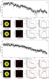 |
Fig. 1 A comparison between the commonly used flux-weighted centroid (FWC) method (labelled a) and the mean profile-fitting (MPF) method used in this work (labelled b). A particularly small aperture is used in this figure to highlight the differences between the two. Panels i: raw lightcurves obtained from each method. Panels ii and iii: two example PSFs with overlaid apertures. Panels from left to right: image of the PSF overlaid with the chosen aperture (white), the aperture subtracted from the PSF, the mean profile of the PSF window in the X-direction and the mean profile of the PSF window in the Y -direction. The gray vertical lines represent the detected center of the PSF for each different profile, while the dashed lines show the placement of the aperture. The red lines in panels iib and iiib show the profile that was detected using the MPF method. |
3.2 Optimising aperture radii and reference star choices
Differences between the results of repeat analyses is an issue in exoplanet occultation studies (e.g. Evans et al. 2015). The main problem is that the relationship between eclipse depth and the choice of aperture radii and reference stars is often not thoroughly investigated. These two factors can occasionally have a large effect on the resulting eclipse depth and can therefore directly influence inferences that we can make about exoplanetary atmospheres. Croll et al. (2015) puts forward a method that allows the extent to which these parameters influence the eclipse depth to be explored. We use a very similar method to fully explore this relationship for the WASP-48b Ks -band reduction. We outline the steps of the routine below.
1. Source detection. We use SEP, a python Source Extractor Package (Barbary 2016; Bertin & Arnouts 1996), to detect all reference stars within the image. The location of the target star was input manually. As the telescope had been defocused, the non-Gaussian PSF’s caused the source detection algorithm to fail. As a solution, we first calculated and subtracted the background from the image using SEP. We then convolved the remaining image with a PSF kernel, which was pre-selected from the WASP-48b CFHT images, with the requirements of having a high total flux and an absence of bad pixels. This resulted in an image containing Gaussian-like PSFs that was then used with the SEP package to return the coordinates of all stellar PSFs within the image.
2. Aperture photometry. We used the aperture photometry method from Sect. 3.1 to perform photometry with a wide range of apertures for the target star and the detected reference stars. For WASP-48b, we used aperture radii of sizes between 15 and 25 pixels in steps of 0.25 and recorded the flux of 40 reference stars.
3. Initial reference star ranking. We created initial differential lightcurves consisting of the target star, divided by each reference star, for every aperture size. We analysed each of these lightcurves individually in a global Markov chain Monte Carlo analysis (MCMC; see Sect. 3.3), with all transit and radial velocity data from Sect. 3.3, to produce an occultation model. We then used RMS × β2 to calculate the residual scatter of each lightcurve, where β is a parameter that provided an estimate of the correlated noise within the time-series data (Winn et al. 2008). All reference stars were then ranked in order of the lowest RMS × β2 and the best seven were selected for further analysis.
4. Combinedreference star lightcurves. We then combined the selected reference stars to produce further differential lightcurves with potentially lower residual scatter. They consisted of the median-combined lightcurves for every possible combination of the best reference stars and aperture sizes. We once again performed a full, global MCMC to produce an occultation model and used the residual RMS × β2 to rank the lightcurves.
5. Eclipse depth dependencies. Figure 2a shows the determined RMS × β2 as a function of aperture size and number of reference stars. Similar to Croll et al. (2015), we selected the best aperture radii and reference star ensemble by selecting all output lightcurves that produce an RMS × β2 less than 15% above the minimum RMS × β2. This was an arbitrary number, used by Croll et al. (2015), but we also find that this value gives a reasonable representation of the lowest region of RMS × β2 in Fig. 2a. Figure 2b shows how the eclipse depth varies for the same aperture radii and reference star ensembles. For WASP-48b, there was little correlation between the RMS × β2 and the eclipse depth for sensible aperture choices. This indicated that the determined eclipse depth is relatively independant of the choice of these two factors.
6. Combining outputs. As a final step, we combined the output posterior distributions from the MCMCs of the lightcurves that showed the lowest RMS × β2. For these initial MCMCs, excluding occultation lightcurves from other sources, we calculated an eclipse depth of 0.138 ± 0.014% at a phase of 0.4998 ± 0.0010 in the Ks -band. The lightcurves and models for these are shown in Fig. 3.
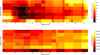 |
Fig. 2 Top: percentage of RMS × β2 above the minimum value shown as a function of aperture size and the number of included reference stars. Bottom: percentage eclipse depth as a function of aperture size and number of reference stars. In both cases, the blue contours indicate the region that contains all values less than 15% above the minimum RMS × β2. |
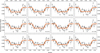 |
Fig. 3 The twelve WASP-48b Ks-band occultation lightcurves that show the lowest RMS × β2, created by different combinations of reference stars and aperture sizes. The data are binned in intervals of 10 min, with the orange model indicating the MCMC fitted solution for that particular aperture and reference star combination. The caption within the figure lists the number of reference stars and aperture size, respectively. |
3.3 Modelling the transit, occultation and orbit
To determine the parameters of the system, we used an adaptive MCMC code (Collier Cameron et al. 2007; Pollacco et al. 2008; Anderson et al. 2015). As well as the initial MCMCs mentioned in Sect. 3.1, we also performed a final global MCMC for each of the lightcurves that produced the lowest RMS × β2 in Sect. 3.2. These final MCMCs used an additional 4 occultation lightcurves as well as 5 transit lightcurves and 14 radial velocities from SOPHIE (E11) as inputs. We then combined the posteriors of every MCMC and took the median and MAD of the distributions as the parameter values and uncertainties.
The transit lightcurves available for WASP-48b included the LT/RISE and WASP lightcurves from the discovery paper (E11), an ingress observed with the Faulkes Telescope North (hitherto unpublished), the single transit of Sada et al. (2012), 34 transits from the Exoplanet Transit Database2 (Poddaný et al. 2010) and all 10 transits from Ciceri et al. (2015, hereafter C15). We performed an initial MCMC fit to each lightcurve using the model of Mandel & Agol (2002) and the four-parameter, non-linear limb darkening law of Claret (2000, 2004). We rejected transits with high scatter or with significant gaps in the data during the observation. We then selected transits based upon their residual rms, which resulted in 5 transits (the LT/RISE transit from E11, and four transitsfrom C15) being used in the final MCMC runs (Table 1 and Fig. 4).
The occultation data consisted of our CFHT Ks-band lightcurves and the H-band, Ks -band, 3.6- and 4.5-μm lightcurves from O’Rourke et al. (2014). The H-band and Ks-band observationsof O’Rourke et al. (2014) were made using the Palomar 200-inch Hale telescope. These observations may have suffered from the reference star and aperture size degeneracies noted in Sect. 3.2, but given that the raw data was not publicly available, we used the processed data from O’Rourke et al. (2014) in our final MCMCs. The 3.6-μm and 4.5-μm observationswere made using the Spitzer space telescope. For each MCMC, we fit both of the specific CFHT Ks -band lightcurve and the Palomar Ks-band lightcurve with a single model.
Our MCMC code allows the detrending of both transit and occultation lightcurves against multiple parameters. We detrended all transit lightcurves with a quadratic function of time as it led to a decrease in the residual rms scatter over linear detrending or not detrending. We detrended against detector position for the Spitzer lightcurves and against linear time for the Palomar data. We chose the model with which to detrend our Ks -band CFHT lightcurve using the Bayesian information criterion (Schwarz 1978), which penalises model complexity. We investigated possible dependencies on time, airmass, detector position, sky background and FWHM, in various combinations, but we found that a linear function of time alone resulted in a significant improvement in the final RMS × β2.
The freeparameters we used in our MCMC code are listed in Table 2 as “proposal” parameters. We obtained values of stellar mass (1.113 ± 0.084M⊙) and age (6.5 ± 1.7 Gyr) from a comparison with stellar models using the BAGEMASS code of Maxted et al. (2015). We used inputs of Teff = 6000 ± 150 K and [Fe/H] = 0.12 ± 0.12 from the spectral analysis of E11 and ρ* = 0.276 ± 0.018 ρ⊙ from an initial MCMC run. At each step in our MCMC analysis, we drew a value of M* from a normal distribution with mean and standard deviation equal to the BAGEMASS-derived values.
We present the median values and the 1σ limits of ourfinal MCMC parameters’ combined posterior distributions in Table 2. We plot the corresponding models along with the transit lightcurves in Fig. 4 and the detrended occultation lightcurves in Fig. 5.
We updated the system parameters by analysing the five highest quality transits together with all the available radial velocities and occultation lightcurves. In Table 3, we compare some key system parameters from our solution with those of E11 and C15. We obtained a stellar density that is 1σ lower than C15. This resulted in a stellar mass, via evolutionary models, ~ 0.4σ larger than found by C15. In turn, our stellar radius is 1σ larger than that of C15. As we both found similar transit depths our planetary radius is also larger by 1σ. The radius we derived for WASP-48b is consistent with that predicted by the empirical relation of Enoch et al. (2012) based on the planet’s mass, irradiation and host-star metallicity (1.51 ± 0.04 RP).
We checked whether any single lightcurve could have biased the time of mid-occultation, and therefore the occultation depths of the other bands, in our global solution. The occultation mid-points and depths from MCMCs in which we fit only one occultation lightcurve are consistent with those obtained from the final MCMCs (Table 4).
The Ks-band occultation depth (0.109± 0.027%) of O’Rourke et al. (2014) is consistent with our fit to their data (0.108 ± 0.026%) and with the depth from the fit to our Ks-band data alone (0.138 ± 0.014%) as well as the global solution (0.136 ± 0.014%). We found that the timing offset of the eclipse for the global solution (0.9 ± 1.9 mins) was consistent with the timing offset produced from the MCMCs in Sect. 3.2, using the CFHT occultation alone (− 0.3 ± 2.2 mins). The values of e cosω are also in good agreement, with values of 0.00046 ± 0.00091 and 0.00000 ± 0.00103 for the global and CFHT Ks -band MCMCs respectively. This demonstrates that our Ks-band data is able to solely constrain the timing of the occultation.
From an analysis of the radial-velocity data and limited transit data, E11 found the eccentricity of the orbit to be small and consistent with zero: 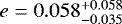 . The addition of our occultation lightcurves results in a far tighter constraint on eccentricity (Fig. 6), and more so with the addition of the four occultation lightcurves of O’Rourke et al. (2014). Thus we find e < 0.008 at the 1σ level and e < 0.072 at the 3σ level.
Transit lightcurves used in our MCMC analysis.
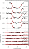 |
Fig. 4 Upperpanel: transit lightcurves, detrended as described in the text, and the best-fitting transit model from our MCMC analysis. See Table 1 for a key. The lightcurves are binned to 2 min intervals for comparison. Lower panel: residuals about the fits. |
Orbital, stellar and planetary parameters from the MCMC analysis.
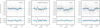 |
Fig. 5 Occultation lightcurves from O’Rourke et al. (2014), detrended as described in Sect. 3.3. The best-fitting occultation models from our global MCMC analysis are plotted in blue. The black points with error bars show the data binned in 20 min intervals. Bottom row: binned residuals about the fits. |
A comparison between our solution and the literature.
Occultation depths and mid-occultation phases of WASP-48.
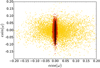 |
Fig. 6 Posterior distributions of esinω and e cosω for different subsets of data (represented by different colours). We plot the results from analysing transit lightcurves and radial velocities alone (yellow), when including our Ks -band occultation lightcurves (red) and when the four occultation lightcurves of O’Rourke et al. (2014) were also included (black). |
3.4 Checking the effects of time-correlated noise
Time-correlated noise can produce variations in lightcurves with similar amplitudes to occultations meaning the measurements of the latter could be affected. We estimated the levels and timescales of red noise in the occultation lightcurves by comparing the residual scatter with the white-noise expectation for a range of temporal bin sizes (Fig. 7). This suggested that red noise could be significant in both of the Palomar lightcurves and in the Spitzer 3.6-μm lightcurve.
We investigated the effect of red noise on our measurements of the occultation depth and mid-point using the residual permutations or “Prayer-Bead” method (Gillon et al. 2009; Winn et al. 2009). We sequentially shifted the residuals from each of our detrended occultation lightcurves before adding back the model and trend function, such that we end up with as many lightcurves as there are data points. Thus the temporal structure of any red noise was preserved. We then applied our MCMC code to each of these lightcurves. We plot the distributions of the occultation depths in Fig. 8 and give the median and 1σ limits of thedistributions of occultation depth and mid-point in the final two columns of Table 4. From the close agreement with the values of the final MCMCs, we conclude that red noise does not significantly affect our results, therefore we adopt the final MCMC solution (Table 2).
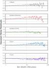 |
Fig. 7 Residual rms vs. bin width as compared to the white-noise expectation. This is similar to the common rms vs. bin-width plot (e.g. Fig. 6 of Hardy et al. 2017), but we have divided throughout by the white-noise prediction such that deviations from this level are clearer. |
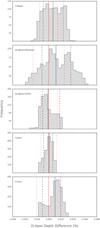 |
Fig. 8 Distributions of occultation depth produced by the residual permutations method. In each case, the value from the final MCMCs (solid red line) has been subtracted; the dashed red lines are the MCMC 1σ limits. The solid and the dashed black lines are the medians and the 1σ confidence intervals of the residual-permutations distributions. |
4 Atmospheric analysis
We investigate possible constraints on the thermal structure and chemical composition of the day-side atmosphere of WASP-48b by comparing the planet-to-star flux ratios of Table 2 with atmospheric models. The H-band and Ks -band, due to their lack of strong spectral features, are spectral windows that probe the temperature profile in the deep atmosphere of the planet, which is expected to be isothermal for pressures above ~1 bar (Madhusudhan 2012). On the other hand, the Spitzer 3.6- and 4.5-μm bands span spectral features due to several molecules and hence probe temperatures at different altitudes in the atmosphere. Importantly, these two bandpasses are particularly useful for constraining thermal inversions in hot Jupiters as, for solar composition atmospheres, the presence of a strong thermal inversion is expected to result in significantly higher thermal emission at 4.5 μm than at 3.6 μm due to strong CO emission (Burrows et al. 2007, 2008; Fortney et al. 2008; Madhusudhan & Seager 2010).
We model the day-side emergent spectrum of WASP-48b using the atmospheric modelling and retrieval method of Madhusudhan & Seager (2009) and Madhusudhan (2012). The model computes line-by-line radiative transfer in a plane-parallel (1-D) atmosphere assuming hydrostatic equilibrium, local thermodynamic equilibrium (LTE), and global energy balance. We assume a Kurucz model for the stellar spectrum (Castelli & Kurucz 2004) appropriate to the stellar parameters. The pressure–temperature (P–T) profile and molecular volume mixing ratios are free parameters in the model. The P–T profile comprises of six free parameters and the volume mixing ratio of each molecular species, assumed to be uniformly mixed in the atmosphere, constitutes an additional free parameter. We include the dominant sources of opacity expected in hot Jupiter atmospheres, namely, molecular line absorption due to H2 O, CO, CO2, CH4, C2 H2, HCN, TiO, and VO (see e.g. Madhusudhan 2012; Moses et al. 2013) and H2 –H2 collision-induced absorption (Borysow 2002). The generality of the parametric P–T profile and the range of molecules included allow us to exhaustively explore the model parameter space, including models with and without thermal inversions and those with oxygen-rich vs. carbon-rich compositions. However, given the limited number of observations available, our goal in the present work is not to find a unique model fit to the data, but instead to constrain the regions of atmospheric parameter space that are allowed or ruled out by the data.
We find that current data provide only marginal constraints on the presence of a thermal inversion in the day-side atmosphere of WASP-48b. The observations and two model spectra are shown in Fig. 9. Both models have a solar abundance composition in chemical equilibrium (Burrows & Sharp 1999; Madhusudhan 2012) but with very different temperature profiles, one with a thermal inversion and the other without. Both profiles produce a model that is consistent with the data, but the model without a thermal inversion provides a marginally better fit. In the non-inverted model, the spectral features are caused by molecular absorption due to the temperature decreasing with altitude above the planetary photosphere at ~1 bar. The peaks in the H and Ks bands and in part of the 3.6-μm band show continuum emission from the photosphere due to the lack of significant molecular features at those wavelengths. The molecular features in the 3.6- and 4.5-μm bands are caused predominantly by H2O and CO. In contrast, in the inversion model, the peaks in the spectra are caused by molecular emission features due to the same molecules, H2 O and CO, whereas the troughs represent the continuum emission from the photosphere. The H-band and Ks -band points very well constrain the isothermal temperature profile in the lower atmosphere to be ~2300 K, regardless of the presence/absence of an inversion in the upper atmosphere. The error bar on the 4.5-μm measurement, which is crucial to constrain the thermal inversion, makes it hard to distinguish between the two models. Moreover, a featureless blackbody spectrum of ~2100 K, as shown by the central dotted curve, also provides a reasonable match to the data, further confirming the inability of the data to constrain the temperature profile in the upper atmosphere. Finally, while solar composition models as shown here provide a very good match to the current data the actual composition is largely unconstrained due to degeneracy with the inconclusive temperatureprofile.
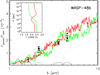 |
Fig. 9 A comparison of the planet-to-star contrast ratios of WASP-48b with model spectra. The red line depicts a model with a thermal inversion and the green line is for a model without an inversion. The black points show the contrast ratios from our analysis (Table 2) and the coloured points show the band-integrated values of the two models. The transmission curves of each filter are plotted in black, though the CFHT Ks -band is plotted in blue and the black dotted line is the Palomar Ks-band. The similarity between the two enables us to analyse them together. The inset plot shows the pressure–temperature profiles of the two models. The three dashed lines are black bodies with temperatures of 1500, 2100 and 2500 K. |
5 Discussion
We have detected the thermal emission of WASP-48b in the Ks -band, finding a planet-to-star contrast ratio of 0.136 ± 0.014%. By optimising the selection of aperture radii and reference star choices, using a calibration pipeline that is optimised for ground-based occultation photometry and using a new centering method, we found a significant improvement in the quality of lightcurve that is produced. Compared to traditional methods, the RMS scatter of the final lightcurves were reduced by ~ 30%.
We combined our results with existing infrared measurements to investigate the planet’s atmosphere. We found that the current datamarginally favour an atmosphere without a thermal inversion, but are also compatible with its presence. There are a number of similar cases, where the data are unable to strongly constrain the presence of a temperature inversion (Knutson et al. 2008; Désert et al. 2011; Smith et al. 2012; Todorov et al. 2013; Line et al. 2016; Hardy et al. 2017). In fact, even for well studied atmospheres, the detection of a thermal inversion can be ambiguous. The first temperature inversion in the atmosphere of a hot Jupiter was claimed for HD 209458 b, which became the archetype (Knutson et al. 2008). However, recent studies based on new data and a reanalysis of existing data have found no evidence for a strong temperature inversion (Diamond-Lowe et al. 2014; Schwarz et al. 2015; Line et al. 2016). Confirming the presence of a thermal inversion can be difficult because there is often a degeneracy caused by the limited number of SED data points and the degrees of freedom allowed by the molecular abundances in model spectra (Madhusudhan & Seager 2009). The precision of the contrast ratios is also a factor in distinguishing between models. Specifically, a higher precision measurement at 4.5-μm would help to discriminate between the two scenarios in Fig. 9. Also, as photometric bandpasses can average over multiple molecular features, small inversions can often be masked. High-precision spectroscopic observations, such as those in Deming et al. (2013), will ultimately be required to place stringent constraints on the temperature profile as well as chemical composition of the atmosphere of WASP-48b. Murgas et al. (2017) performed such observations of WASP-48b with the ground-based OSIRIS spectrograph on the 10.4 m Gran Telescopio Canarias telescope. They obtained a flat, featureless optical transmission spectrum of WASP-48b that agreed with a cloud-free atmosphere including the presence of titanium oxide and vanadium oxide. However, the result was not statistically significant enough to claim a detection of either molecule.
We find a Ks-band eclipse depth similar to that of O’Rourke et al. (2014). Our Ks-band depth is 0.029% larger than the value that they report, which in comparison to their 0.027% reported uncertainty indicates that there is little variation between the two measurements. This rules out large temperature variations or violent storms on short timescales in the atmosphere of WASP-48b at the deep regions that the Ks -band is able to examine. Our result also helps to place a limit on the systematics of these types of ground-based observations; despite using a different telescope and detector, as well as a different reduction method, we have measured a Ks -band eclipse depth that agrees with O’Rourke et al. (2014) to the 1σ level. However, this is not the case for all repeat occultation analysis that have been performed from ground-based instruments. For example the Ks-band measurements of TRES-3b preformed by de Mooij & Snellen (2009) and Croll et al. (2010) were discrepant by ≳ 2σ, which Croll et al. (2010) note, is best explained by the impact of systematic uncertainties in the observations of de Mooij & Snellen (2009).
It is important to ensure that transit and occultation analyses are robust and produce repeatable eclipse depths. We believe that the method put forward by Croll et al. (2015), and used in this work, sufficiently explores the effects that choices in aperture size and companion stars have on the final result. As well as this, we have tested for the presence of correlated noise and determined that it has little effect on the resulting eclipse depth. By ruling out factors such as these, the eclipse depths produced should be reliable and enable us to make accurate deductions about exoplanets and their atmospheres.
Acknowledgements
The research leading to these results has received funding from the European Union Seventh Framework Programme (FP7/2013-2016) under grant agreement No. 312430 (OPTICON; proposal 2012A016). Based on observations obtained with WIRCam under program 12AO16, a joint project of CFHT, Taiwan, Korea, Canada, France, at the Canada-France-Hawaii Telescope (CFHT) which is operated by the National Research Council (NRC) of Canada, the Institut National des Sciences de l’Univers of the Centre National de la Recherche Scientifique of France, and the University of Hawaii. We are grateful to the observers listed in Table 1 for making available their transit lightcurves. AMSS acknowledges support from the Polish NCN through grant no. 2012/07/B/ST9/04422. We also thank the referee for their helpful comments on the previous versions of this publication.
References
- Agol, E., Cowan, N. B., Knutson, H. A., et al. 2010, ApJ, 721, 1861 [NASA ADS] [CrossRef] [Google Scholar]
- Anderson, D. R., Smith, A. M. S., Madhusudhan, N., et al. 2013, MNRAS, 430, 3422 [NASA ADS] [CrossRef] [EDP Sciences] [Google Scholar]
- Anderson, D. R., Collier Cameron, A., Hellier, C., et al. 2015, A&A, 575, A61 [NASA ADS] [CrossRef] [EDP Sciences] [Google Scholar]
- Armstrong, D. J., de Mooij, E., Barstow, J., et al. 2016, Nat. Astron., 1, 4 [Google Scholar]
- Barbary, K. 2016, Journal of Open Source Software, 1(6), 58 [NASA ADS] [CrossRef] [Google Scholar]
- Bean, J. L., Désert, J.-M., Seifahrt, A., et al. 2013, ApJ, 771, 108 [NASA ADS] [CrossRef] [Google Scholar]
- Bertin, E., & Arnouts, S. 1996, A&AS, 117, 393 [NASA ADS] [CrossRef] [EDP Sciences] [Google Scholar]
- Borysow, A. 2002, A&A, 390, 779 [NASA ADS] [CrossRef] [EDP Sciences] [Google Scholar]
- Burrows, A., & Sharp, C. M. 1999, ApJ, 512, 843 [NASA ADS] [CrossRef] [Google Scholar]
- Burrows, A., Hubeny, I., Budaj, J., Knutson, H. A., & Charbonneau, D. 2007, ApJ, 668, L171 [NASA ADS] [CrossRef] [MathSciNet] [Google Scholar]
- Burrows, A., Budaj, J., & Hubeny, I. 2008, ApJ, 678, 1436 [NASA ADS] [CrossRef] [Google Scholar]
- Castelli, F., & Kurucz, R. L. 2004, Proc. IAU Symp., 210, Poster A20 [Google Scholar]
- Charbonneau, D., Allen, L. E., Megeath, S. T., et al. 2005, ApJ, 626, 523 [NASA ADS] [CrossRef] [Google Scholar]
- Ciceri, S., Mancini, L., Southworth, J., et al. 2015, A&A, 577, A54 [NASA ADS] [CrossRef] [EDP Sciences] [Google Scholar]
- Claret, A. 2000, A&A, 363, 1081 [NASA ADS] [Google Scholar]
- Claret, A. 2004, A&A, 428, 1001 [NASA ADS] [CrossRef] [EDP Sciences] [Google Scholar]
- Collier Cameron, A., Wilson, D. M., West, R. G., et al. 2007, MNRAS, 380, 1230 [NASA ADS] [CrossRef] [Google Scholar]
- Croll, B., Jayawardhana, R., Fortney, J. J., Lafrenière, D., & Albert, L. 2010, ApJ, 718, 920 [NASA ADS] [CrossRef] [Google Scholar]
- Croll, B., Albert, L., Jayawardhana, R., et al. 2015, ApJ, 802, 28 [NASA ADS] [CrossRef] [Google Scholar]
- Delrez, L., Santerne, A., Almenara, J.-M., et al. 2016, MNRAS, 458, 4025 [NASA ADS] [CrossRef] [Google Scholar]
- Deming, D., Seager, S., Richardson, L. J., & Harrington, J. 2005, Nature, 434, 740 [NASA ADS] [CrossRef] [PubMed] [Google Scholar]
- Deming, D., Wilkins, A., McCullough, P., et al. 2013, ApJ, 774, 95 [NASA ADS] [CrossRef] [Google Scholar]
- de Mooij, E. J. W., & Snellen, I. A. G. 2009, A&A, 493, L35 [NASA ADS] [CrossRef] [EDP Sciences] [Google Scholar]
- Désert, J.-M., Charbonneau, D., Demory, B.-O., et al. 2011, ApJS, 197, 14 [NASA ADS] [CrossRef] [Google Scholar]
- Diamond-Lowe, H., Stevenson, K. B., Bean, J. L., Line, M. R., & Fortney, J. J. 2014, ApJ, 796, 66 [NASA ADS] [CrossRef] [Google Scholar]
- Enoch, B., Anderson, D. R., Barros, S. C. C., et al. 2011, ApJ, 142, 86 [Google Scholar]
- Enoch, B., Collier Cameron, A., & Horne, K. 2012, A&A, 540, A99 [NASA ADS] [CrossRef] [EDP Sciences] [Google Scholar]
- Evans, T. M., Aigrain, S., Gibson, N., et al. 2015, MNRAS, 451, 680 [NASA ADS] [CrossRef] [Google Scholar]
- Fortney, J. J., Lodders, K., Marley, M. S., & Freedman, R. S. 2008, ApJ, 678, 1419 [NASA ADS] [CrossRef] [Google Scholar]
- Gillon, M., Smalley, B., Hebb, L., et al. 2009, A&A, 496, 259 [NASA ADS] [CrossRef] [EDP Sciences] [Google Scholar]
- Hardy, R. A., Harrington, J., Hardin, M. R., et al. 2017, ApJ, 836, 143 [NASA ADS] [CrossRef] [Google Scholar]
- Haynes, K., Mandell, A. M., Madhusudhan, N., Deming, D., & Knutson, H. 2015, ApJ, 806, 146 [NASA ADS] [CrossRef] [Google Scholar]
- Kammer, J. A., Knutson, H. A., Line, M. R., et al. 2015, ApJ, 810, 118 [NASA ADS] [CrossRef] [Google Scholar]
- Knutson, H. A., Charbonneau, D., Allen, L. E., Burrows, A., & Megeath, S. T. 2008, ApJ, 673, 526 [NASA ADS] [CrossRef] [Google Scholar]
- Knutson, H. A., Lewis, N., Fortney, J. J., et al. 2012, ApJ, 754, 22 [NASA ADS] [CrossRef] [Google Scholar]
- Line, M. R., Knutson, H., Wolf, A. S., & Yung, Y. L. 2014, ApJ, 783, 70 [NASA ADS] [CrossRef] [Google Scholar]
- Line, M. R., Stevenson, K. B., Bean, J., et al. 2016, AJ, 152, 203 [NASA ADS] [CrossRef] [Google Scholar]
- Machalek, P., McCullough, P. R., Burke, C. J., et al. 2008, ApJ, 684, 1427 [NASA ADS] [CrossRef] [Google Scholar]
- Madhusudhan, N. 2012, ApJ, 758, 36 [NASA ADS] [CrossRef] [Google Scholar]
- Madhusudhan, N., & Seager, S. 2009, ApJ, 707, 24 [NASA ADS] [CrossRef] [Google Scholar]
- Madhusudhan, N., & Seager, S. 2010, ApJ, 725, 261 [NASA ADS] [CrossRef] [Google Scholar]
- Madhusudhan,N., Knutson, H., Fortney, J., & Barman, T. 2014, in Protostars and Planets VI, eds. H. Beuther, R. S. Klessen, C. P. Dullemond, & T. Henning, (Tucson: University of Arizona Press), 739 [Google Scholar]
- Mandel, K., & Agol, E. 2002, ApJ, 580, L171 [NASA ADS] [CrossRef] [Google Scholar]
- Maxted, P. F. L., Serenelli, A. M., & Southworth, J. 2015, A&A, 575, A36 [NASA ADS] [CrossRef] [EDP Sciences] [Google Scholar]
- McLean, A., Mitchell, C., & Swanston, D. 1994, J. Electron Spectrosc. Relat. Phenomena, 69, 125 [Google Scholar]
- Moses, J. I., Line, M. R., Visscher, C., et al. 2013, ApJ, 777, 34 [NASA ADS] [CrossRef] [Google Scholar]
- Murgas, F., Pallé, E., Parviainen, H., et al. 2017, A&A, 605, A114 [NASA ADS] [CrossRef] [EDP Sciences] [Google Scholar]
- Olivero, J. 1977, J. Quant. Spectr. Rad. Transf., 17, 233 [NASA ADS] [CrossRef] [Google Scholar]
- O’Rourke, J. G., Knutson, H. A., Zhao, M., et al. 2014, ApJ, 781, 109 [NASA ADS] [CrossRef] [Google Scholar]
- Poddaný, S., Brát, L., & Pejcha, O. 2010, New Ast., 15, 297 [Google Scholar]
- Pollacco, D., Skillen, I., Collier Cameron, A., et al. 2008, MNRAS, 385, 1576 [NASA ADS] [CrossRef] [Google Scholar]
- Puget, P., Stadler, E., Doyon, R., et al. 2004, SPIE Conf. Ser., 5492, 978 [Google Scholar]
- Rauscher, E., Menou, K., Cho, J. Y.-K., Seager, S., & Hansen, B. M. S. 2007, ApJ, 662, L115 [NASA ADS] [CrossRef] [Google Scholar]
- Sada, P. V., Deming, D., Jennings, D. E., et al. 2012, PASP, 124, 212 [NASA ADS] [CrossRef] [Google Scholar]
- Schwarz, G. 1978, Ann. Stat., 6, 461 [NASA ADS] [CrossRef] [MathSciNet] [Google Scholar]
- Schwarz, H., Brogi, M., de Kok, R., Birkby, J., & Snellen, I. 2015, A&A, 576, A111 [NASA ADS] [CrossRef] [EDP Sciences] [Google Scholar]
- Shporer, A., O’Rourke, J. G., Knutson, H. A., et al. 2014, ApJ, 788, 92 [NASA ADS] [CrossRef] [Google Scholar]
- Smith, A. M. S., Anderson, D. R., Madhusudhan, N., et al. 2012, A&A, 545, A93 [NASA ADS] [CrossRef] [EDP Sciences] [Google Scholar]
- Stevenson, K. B., Désert, J.-M., Line, M. R., et al. 2014, Science, 346, 838 [NASA ADS] [CrossRef] [Google Scholar]
- Todorov, K. O., Deming, D., Knutson, H. A., et al. 2013, ApJ, 770, 102 [NASA ADS] [CrossRef] [Google Scholar]
- Vida, K., Kővári, Z., Pál, A., Oláh, K., & Kriskovics, L. 2017, ApJ, 841, 124 [NASA ADS] [CrossRef] [Google Scholar]
- Wheatley, P. J., Collier Cameron, A., Harrington, J., et al. 2010, ApJ, submitted [arXiv:1004.0836] [Google Scholar]
- Winn, J. N., Holman, M. J., Torres, G., et al. 2008, ApJ, 683, 1076 [NASA ADS] [CrossRef] [Google Scholar]
- Winn, J. N., Holman, M. J., Henry, G. W., et al. 2009, ApJ, 693, 794 [NASA ADS] [CrossRef] [Google Scholar]
- Zellem, R., Griffith, C. A., Lewis, N. K., Swain, M. R., & Knutson, H. A. 2014, in AAS/Division for Planetary Sciences Meeting Abstracts, 46, 104.04 [NASA ADS] [Google Scholar]
All Tables
All Figures
|
Fig. 1 A comparison between the commonly used flux-weighted centroid (FWC) method (labelled a) and the mean profile-fitting (MPF) method used in this work (labelled b). A particularly small aperture is used in this figure to highlight the differences between the two. Panels i: raw lightcurves obtained from each method. Panels ii and iii: two example PSFs with overlaid apertures. Panels from left to right: image of the PSF overlaid with the chosen aperture (white), the aperture subtracted from the PSF, the mean profile of the PSF window in the X-direction and the mean profile of the PSF window in the Y -direction. The gray vertical lines represent the detected center of the PSF for each different profile, while the dashed lines show the placement of the aperture. The red lines in panels iib and iiib show the profile that was detected using the MPF method. |
| In the text | |
|
Fig. 2 Top: percentage of RMS × β2 above the minimum value shown as a function of aperture size and the number of included reference stars. Bottom: percentage eclipse depth as a function of aperture size and number of reference stars. In both cases, the blue contours indicate the region that contains all values less than 15% above the minimum RMS × β2. |
| In the text | |
|
Fig. 3 The twelve WASP-48b Ks-band occultation lightcurves that show the lowest RMS × β2, created by different combinations of reference stars and aperture sizes. The data are binned in intervals of 10 min, with the orange model indicating the MCMC fitted solution for that particular aperture and reference star combination. The caption within the figure lists the number of reference stars and aperture size, respectively. |
| In the text | |
|
Fig. 4 Upperpanel: transit lightcurves, detrended as described in the text, and the best-fitting transit model from our MCMC analysis. See Table 1 for a key. The lightcurves are binned to 2 min intervals for comparison. Lower panel: residuals about the fits. |
| In the text | |
|
Fig. 5 Occultation lightcurves from O’Rourke et al. (2014), detrended as described in Sect. 3.3. The best-fitting occultation models from our global MCMC analysis are plotted in blue. The black points with error bars show the data binned in 20 min intervals. Bottom row: binned residuals about the fits. |
| In the text | |
|
Fig. 6 Posterior distributions of esinω and e cosω for different subsets of data (represented by different colours). We plot the results from analysing transit lightcurves and radial velocities alone (yellow), when including our Ks -band occultation lightcurves (red) and when the four occultation lightcurves of O’Rourke et al. (2014) were also included (black). |
| In the text | |
|
Fig. 7 Residual rms vs. bin width as compared to the white-noise expectation. This is similar to the common rms vs. bin-width plot (e.g. Fig. 6 of Hardy et al. 2017), but we have divided throughout by the white-noise prediction such that deviations from this level are clearer. |
| In the text | |
|
Fig. 8 Distributions of occultation depth produced by the residual permutations method. In each case, the value from the final MCMCs (solid red line) has been subtracted; the dashed red lines are the MCMC 1σ limits. The solid and the dashed black lines are the medians and the 1σ confidence intervals of the residual-permutations distributions. |
| In the text | |
|
Fig. 9 A comparison of the planet-to-star contrast ratios of WASP-48b with model spectra. The red line depicts a model with a thermal inversion and the green line is for a model without an inversion. The black points show the contrast ratios from our analysis (Table 2) and the coloured points show the band-integrated values of the two models. The transmission curves of each filter are plotted in black, though the CFHT Ks -band is plotted in blue and the black dotted line is the Palomar Ks-band. The similarity between the two enables us to analyse them together. The inset plot shows the pressure–temperature profiles of the two models. The three dashed lines are black bodies with temperatures of 1500, 2100 and 2500 K. |
| In the text | |
Current usage metrics show cumulative count of Article Views (full-text article views including HTML views, PDF and ePub downloads, according to the available data) and Abstracts Views on Vision4Press platform.
Data correspond to usage on the plateform after 2015. The current usage metrics is available 48-96 hours after online publication and is updated daily on week days.
Initial download of the metrics may take a while.