| Issue |
A&A
Volume 577, May 2015
|
|
|---|---|---|
| Article Number | A78 | |
| Number of page(s) | 53 | |
| Section | Extragalactic astronomy | |
| DOI | https://doi.org/10.1051/0004-6361/201425359 | |
| Published online | 06 May 2015 | |
Star-formation histories of local luminous infrared galaxies⋆,⋆⋆
1 Centro de Astrobiología
(CSIC/INTA), Ctra de Torrejón a
Ajalvir, km 4, 28850 Torrejón
de Ardoz, Madrid,
Spain
e-mail: mpereira@cab.inta-csic.es
2 Instituto de Física de Cantabria,
CSIC-Universidad de Cantabria, 39005
Santander,
Spain
3 Departamento de Física Teórica,
Universidad Autónoma de Madrid, 28049
Madrid,
Spain
4 Departamento de Astrofísica, Facultad
de CC. Físicas, Universidad Complutense de Madrid, 28040
Madrid,
Spain
5 Cavendish Laboratory, University of
Cambridge 19 J. J. Thomson Avenue, Cambridge
CB3 0HE,
UK
6 Spitzer Science Center, California
Institute of Technology, MS
220-6, Pasadena,
CA
91125,
USA
7 Núcleo de Astronomía de la Facultad
de Ingeniería, Universidad Diego Portales, Av. Ejército Libertador 441, Santiago, Chile
Received: 18 November 2014
Accepted: 16 February 2015
We present analysis of the integrated spectral energy distribution (SED) from the ultraviolet (UV) to the far-infrared and Hα of a sample of 29 local systems and individual galaxies with infrared (IR) luminosities between 1011L⊙ and 1011.8L⊙. We combined new narrow-band Hα + [N ii] and broad-band g, r optical imaging taken with the Nordic Optical Telescope (NOT), with archival GALEX, 2MASS, Spitzer, and Herschel data. Their SEDs(photometry and integrated Hα flux) were fitted simultaneously with a modified version of the magphys code using stellar population synthesis models for the UV–near-IR range and thermal emission models for the IR emission taking the energy balance between the absorbed and re-emitted radiation into account. From the SED fits, we derive the star-formation histories (SFH) of these galaxies. For nearly half of them, the star-formation rate appears to be approximately constant during the last few Gyr. In the other half, the current star-formation rate seems to be enhanced by a factor of 3–20 with respect to what occurred ~1 Gyr ago. Objects with constant SFH tend to be more massive than starbursts, and they are compatible with the expected properties of a main-sequence (M-S) galaxy. Likewise, the derived SFHs show that all our objects were M-S galaxies ~1 Gyr ago with stellar masses between 1010.1 and 1011.5 M⊙. We also derived the average extinction (Av = 0.6−3 mag) and the polycyclic aromatic hydrocarbon luminosity to LIR ratio (0.03−0.16) from our fits. We combined the Av with the total IR and Hα luminosities into a diagramthat can be used to identify objects with rapidly changing (increasing or decreasing) SFR during the past 100 Myr.
Key words: galaxies: evolution / galaxies: starburst / galaxies: star formation
Appendices are available in electronic form at http://www.aanda.org
FITS files for all the reduced images are only available at the CDS via anonymous ftp to cdsarc.u-strasbg.fr (130.79.128.5) or via http://cdsarc.u-strasbg.fr/viz-bin/qcat?J/A+A/577/A78
© ESO, 2015
1. Introduction
Galaxies with high infrared (IR) luminosities (LIR = L(8 − 1000 μm) > 1011 L⊙) are rare in the local Universe (e.g., Le Floc’h et al. 2005), and yet they are a cosmologically important class of objects because they dominate the star-formation rate (SFR) density at high-z. They can be classified as luminous (LIR = 1011 − 1012 L⊙) and ultra-luminous (LIR> 1012 L⊙) IR galaxies (LIRGs and ULIRGs, respectively). LIRGs dominate the SFR density at z ~ 1, while ULIRGs do so at z ~ 2 (Pérez-González et al. 2005; Caputi et al. 2007).
The bulk of the IR luminosity of U/LIRGs is produced by strong star-formation (SF) bursts (Sanders & Mirabel 1996), although, the number of U/LIRGs with an active Galactic nuclei (AGN) detected in their optical spectra increases with the IR luminosity, reaching ~50% when LIR> 1012.3 L⊙ (Yuan et al. 2010). Similarly, the relative contribution of AGN to the bolometric luminosity increases with increasing IR luminosity providing less than 2% to 15% of the total luminosity of local LIRGs (Pereira-Santaella et al. 2011; Petric et al. 2011; Alonso-Herrero et al. 2012a) and ~20% to 25% of the luminosity of local ULIRGs (Farrah et al. 2007; Nardini et al. 2009).
These episodes of intense SF and high IR luminosities are mainly triggered by major mergers involving gas-rich progenitors in the case of local ULIRGs (Sanders & Mirabel 1996). Actually, a majority (>80%) of local ULIRGs are mergers (e.g., Veilleux et al. 2002). This is not true for local LIRGs, which have more varied morphologies – isolated disks, disturbed spirals, or mergers (e.g., Arribas et al. 2004; Alonso-Herrero et al. 2006; Hung et al. 2014). Hammer et al. (2005) suggest that episodic SF bursts due to minor mergers (or gas infall) could enhance the IR luminosity above the LIRG threshold. Moreover, according to N-body simulations, the most likely remnants of these minor interactions are disturbed spirals (Bournaud et al. 2007). This scenario seems to describe the observed morphologies of local LIRGs well.
High-z ULIRGs differ from local objects with similar luminosities for several reasons. First, the incidence of mergers in high-z ULIRGs is lower than locally, with only 30% to 40% of the z> 1 ULIRGs showing merger morphologies (e.g., Elbaz et al. 2007; Kartaltepe et al. 2010). In addition, the mid-IR spectra of z ~ 2 ULIRGs differ from those of local ULIRGs because they are more similar to those local LIRGs (Farrah et al. 2008; Rigby et al. 2008). Therefore, the triggering mechanisms and the physical conditions of the SF in distant ULIRGs resemble those of local LIRGs. In this context, the detailed study of local LIRGs is needed to better understand their high-z counterparts.
In this work we model the integrated spectral energy distribution (SED) of a sample of local IR bright galaxies and derive fundamental physical parameters such as the stellar mass, SFR, star-formation history (SFH), average extinction, etc. The analysis of the integrated emission of local LIRGs is important for providing meaningful comparisons with the integrated SED used in high-z studies. Previous works of the integrated SED of nearby galaxies focus on lower luminosity galaxies (e.g., Noll et al. 2009; Skibba et al. 2011; Brown et al. 2014) or higher luminosity U/LIRGs (e.g., da Cunha et al. 2010; U et al. 2012), which shows that studying intermediate luminosity objects is needed.
The paper is organized as follows. In Sect. 2 the sample of local LIRGs is presented. Sections 3 and 4 describe the data reduction and the models used for the SED fitting, respectively.In Sect. 5 we discuss the SFH of this sample and the age effects on the Hα-to-IR luminosity ratio. Finally, the main conclusions are presented in Sect. 6.
Throughout this paper we assume the following cosmology: H0 = 70 km s-1 Mpc-1, Ωm = 0.3, and ΩΛ = 0.7.
2. Sample
We drew a volume-limited sample of local LIRGs from the IRAS Revised Bright Galaxy Sample (RBGS; Sanders et al. 2003). Our selection criteria are similar to those used by Alonso-Herrero et al. (2006): vhel = 2750−5200 km s-1 and Galactic latitude |b| > 5, but we slightly decreased the minimum LIR down to log LIR/L⊙ = 11.0. There are 59 sources in the RBGS that fulfill these criteria, and 37 of them are observable from the Roque de los Muchachos Obsevatory (Dec > −16°).
We obtained good quality g, r, and narrow-band Hα images for 25 of them using the Nordic Optical Telescope (NOT; see Sect. 3.1), and another four had integrated Hα flux measurements (Moustakas & Kennicutt 2006) and Sloan Digital Sky Survey (SDSS; Aihara et al. 2011) g and r images available. Therefore, our sample includes 29 (78%) of the parent-sample northern LIRGs. Most of the missing galaxies belong to the lower end of the LIR distribution (log LIR/L⊙ ~ 11.0), which is already well represented in our sample (see Table 1).
In addition, we observed six nearby companions of the RBGS objects (namely, NGC 876, UGC 03405, NGC 2389, MCG +02-20-002, NGC 6921, and NGC 7769) with log LIR/L⊙ = 10.2−10.7. They are located between 1−6′ (20 − 100 kpc) away from the main RBGS galaxy and therefore might contribute to the measured IRAS fluxes. We were also able to resolve three of the RBGS targets into two subcomponents (CGCG 468-002 NED01/02, NGC 7752/3, and NGC 7770/1). Our sample contains the 38 sources listed in Table 1.
The IR luminosity range is 1010.2−1011.8 L⊙, with a mean and median luminosity of 1011.0 L⊙. Except for one galaxy, CGCG 468-002 NED01, the IR luminosity is dominated by SF, and the bolometric AGN contribution is small, less than 5% for most galaxies and up to 12% in a few of them (see Table 1 and Alonso-Herrero et al. 2012a).
According to their nuclear activity classification, our sample includes 11 H ii galaxies, 13 composite, one LINER, five Seyfert galaxies, three objects without a clear optical classification1, and one galaxy with no available optical spectrum. For nine of them we determined their nuclear classification and [N ii]6584 Å/Hα ratio using archival optical spectroscopy (see Appendix A). The fraction of galaxies of each type is similar to what is expected for galaxies with IR luminosities in the range covered by our sample (Yuan et al. 2010).
The sample.
3. Observations and data reduction
In this section we describe the reduction and analysis of our new optical observations (Sect. 3.1) along with the archival data (Sect. 3.2). The reduced images for each galaxy are shown in Fig. 1 and Appendix C.
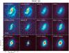 |
Fig. 1 Subset of the images used to construct the integrated SED of NGC 23. The new NOT optical observations of the g, r, and Hα+[N ii] bands are shown. The rest of the images were obtained from the public archives of their respective observatories (see Sect. 3 for details). Some images used in the SED are not displayed here because they have morphologies similar to those of the presented images (2MASS J and H, IRAC 4.5 and 5.8 μm, and PACS 100 μm) or because they have a very low angular resolution (SPIRE 350 and 500 μm). All images are shown in a logarithm scale. North is up and east to the left. The white bar in the Hα+[N ii] panel represents 10 kpc at the distance of the object. |
Log of the NOT/ALFOSC observations.
3.1. Optical imaging
We obtained broad- and narrow-band imaging of 34 IR bright galaxies using the Andalucia Faint Object Spectrograph and Camera (ALFOSC) on the 2.6 m NOT at the Roque de los Muchachos Obsevatory during three observing runs between May and December 2011 (see Table 2)as part of the programs 115-NOT11/11A and 28-NOT2/11B. We used the broad-band SDSS g and r filters (#120 and #110), and for the narrow-band images we used the filters #50 and #68 from the NOT filters set, and #65 and #66 from the Isaac Newton Group of Telescopes (ING). These narrow filters have a full-width half-maximum (FWHM) of about 5 nm and λc between 663 and 665 nm (see Table 3). For three objects (Arp 299, NGC 5936, and NGC 5990) not observed by us with the g filter, we used their available SDSS g image (Aihara et al. 2011). In addition, the r and g images of SDSS were used for IC 860, NGC 5653, Zw 049-057, and NGC 6052.
We selected the narrow-band filter for each galaxy according to its redshift. The plate scale of ALFOSC is 0.19′′ pixel-1, and its field of view (FoV) is 7′×7′, large enough to cover the emission of these LIRGs with a single pointing. The atmospheric conditions were photometric, and the seeing varied between 0.̋6 and 1.̋5 with a median seeing of 0.̋9.
The integration times were 1300 and 800 s for the g and r filters, respectively, and 3000 s for the narrow-band filters. Each integration was divided into three to five dithered exposures that were later combined to correct for cosmic ray hits and bad pixels of the detector.
For the data reduction, we first subtracted the bias level using the overscan region to scale the master bias. During the April run, the bias showed noticeable variability between exposures, so we used the overscan region to estimate the bias level of each row in each exposure. Then the resulting images were divided by the sky flat of the corresponding filter. In addition, bad pixels identified in the flat field images were masked. The sky extinction was determined by observing spectrophotometric standard stars from the ING catalog (ING Technical Note 100) and standard SDSS stars (Smith et al. 2002) at different air masses between 1 and 4. Besides this, we used these standard stars to calculate the photometric AB zero points for the g and r filters.
We combined individual exposures after subtracting the sky background emission and aligning them to a common reference image using stars in the FoV. The absolute astrometry of each image was determined using the Guide Star Catalog (GSC2.3; Lasker et al. 2008). About 10 to 40 stars were used for each image, and the estimated 1σ astrometric uncertainty is 0.̋1−0.̋2. We checked our absolute flux calibration for those fields that were also observed by the SDSS (15 out of 28). We found good agreement between our measurements and those reported in the eighth data release of the SDSS (Aihara et al. 2011) with differences around 0.01−0.05 mag for objects brighter than 19 mag.
We used the Fitzpatrick (1999) extinction law and the Galactic color excess E(B − V) (Table 5) from the NASA/IPAC extragalactic database (NED) to correct the observed optical fluxes for Galactic extinction.
3.1.1. Hα narrow-band imaging calibration
To obtain the Hα+[N ii] emission images, we first subtracted the continuum using the r band image. It was scaled using the relative fluxes of 10−30 field stars observed in both images using 4′′ apertures. These scaling factors are in good agreement with the theoretical factor that can be calculated using the transmission curves of the filters. Some of the nights we obtained observations of standard stars with all the narrow filters, which confirms that the derived scaling factors are accurate within ~15%.
To calculate the conversion factor from counts s-1 in the narrow filter to the corresponding Hα flux in erg cm-2 s-1 units, we first created a synthetic spectrum including only the Hα line and the 6548 and 6584 Å [N ii] transitions at the redshift of each source. For the nuclear regions (~ 3 kpc) where the [N ii]/Hα ratio would be more uncertain because of the nuclear activity, we used the ratios derived from the nuclear spectrum of each target (Table 1). For the extra-nuclear emission we assumed that [N ii]6584 Å/Hα= 0.3, typical of H ii regions (Kennicutt & Kent 1983). The synthetic spectrum was convolved with the transmission curve of the narrow filter, and the result was converted into physical units using the known input Hα flux and the relation between the narrow- and broad-band r calibration (see previous section). The 10σ sensitivity of the images is ~10-16 erg cm-2 s-1, which corresponds to an Hα luminosity of 1037 erg s-1 at the median distance of our galaxies.
Characteristics of the NOT/ALFOSC filters.
3.1.2. Integrated photometry
We defined the apertures to obtain the integrated emission using the NOT r images. In these images, we considered all the pixels above a surface brightness of 23 mag arcsec-1 and fitted an ellipse to them. The resulting elliptical apertures for each galaxy are listed in Table 4. They encompass most of the r emission for all the sources, although in a few cases, some faint H ii regions at large galactocentric distances (r> 15 kpc) lie outside of them. The diameters of the apertures range between 30 and 200′′ with a median diameter of 80′′ and are equivalent to ~20−25 kpc on average.
To perform the photometry in the optical images (r, g, and Hα), we integrated all the emission in the calculated apertures (Table 4) after masking Galactic stars that lie within them. The integrated fluxes are shown in Table 5.
In this paper we use images with a wide range of angular resolutions, from ~1 to 35′′ (see next section). Therefore, to adapt the calculated elliptical apertures we convolved them using a Gaussian with a FWHM equal to the difference between the desired angular resolution and the r resolution (FWHM ~ 1″) subtracted in quadrature.
3.2. Ancillary archival data
To construct the SEDs of our sources, we looked for observations carried out at different wavelengths from the UV to the far-IR. In particular, we used images from GALEX (UV; Martin et al. 2005), 2MASS (near-IR; Skrutskie et al. 2006), Spitzer (mid-IR; Werner et al. 2004), and Herschel (far-IR; Pilbratt et al. 2010), all publicly available in their archives. The reduction and photometry of these archival data is described below.
3.2.1. GALEX UV data
In the GALEX archive we found far-UV (1516 Å) and/or near-UV (2367 Å) observations for 36 out of 38 galaxies in our sample. Most of them belong to the all-sky imaging survey (AIS). The rest are part of the medium imaging survey (MIS), the nearby galaxies survey (NGS), or guest investigator programs. We used the images downloaded from the archive to make the photometric measurements using the apertures described in Sect. 3.1.2 (Table 4) taking into account that the angular resolution of the GALEX images is 4–6′′. As for the optical images, we masked stars inside of the apertures since in some cases they were bright, particularly in the near-UV band. To estimate the background within the apertures, we used the sky background images provided by the GALEX pipeline. Finally to convert from count rates to physical units, we used the conversion factors given in the GALEX Observer’s Guide.
For one of the galaxies without any GALEX data (NGC 1614), we took the near-UV flux from imaging obtained by the optical monitor (OM) onboard XMM-Newton using the UVW2 (2120 Å) filter (Pereira-Santaella et al. 2011).
We corrected the UV fluxes (Table 5) for Galactic extinction using the same method as we used for the optical data (see Sect. 3.1).
3.2.2. 2MASS data
We retrieved the J (1.2 μm), H (1.7 μm), and Ks (2.2 μm) near-IR images of our galaxies from the Two Micron All Sky Survey (2MASS). Most of them were from the 2MASS extended source catalog (Jarrett et al. 2000), although a few objects were part of the 2MASS large galaxy atlas (Jarrett et al. 2003). These downloaded images were already flux-calibrated with an angular resolution of ~2′′.
The photometry on the images was done considering the same elliptical apertures (Table 4) used for the other bands. In general, there is good agreement between our integrated measurements (Table 5) and those reported in the 2MASS catalogs.
3.2.3. Spitzer IRAC and MIPS imaging
In the Spitzer archive we found imaging of our galaxies for the four IRAC bands (at 3.6, 4.5, 5.8, and 8.0 μm; Fazio et al. 2004) and the 24 μm MIPS band (Rieke et al. 2004). We retrieved the basic calibrated data (BCD) for these observations from the Spitzer archive. The BCD processing includes several corrections (e.g., flat field, linearization, and dark subtraction) and flux calibration based on standard stars. We combined these BCD images into mosaics using the version 18 of the MOsaicker and Point source EXtractor (MOPEX) software provided by the SSC using the standard parameters (see the MOPEX User’s Guide for details on the data reduction). The FWHM of the point spread function (PSF) of these images vary between 1.̋7 and 2.̋0 for the IRAC bands, and it is 5.̋9 for the 24 μm MIPS images.
To measure the integrated emission, we used the apertures listed in Table 4 and corrected for the lower angular resolution of the Spitzer images. For the IRAC images we applied the extended source aperture correction or the point source aperture correction for very compact objects (see the IRAC Instrument Handbook). These corrections are about 20% of the measured flux. In the MIPS 24 μm images, some galaxies are very compact, so we applied the point source correction described in the MIPS Instrument Handbook.
MCG +02-20-002/3 were not observed with MIPS, therefore we consider the IRAS 25 μm flux from Surace et al. (2004) as an upper limit because of the limited IRAS angular resolution (1′ at 25 μm) other sources might contribute to the IRAS flux. The measured integrated fluxes are listed in Tables 5 and 6.
Photometry apertures.
3.2.4. Herschel PACS and SPIRE imaging
Far-IR imaging of our galaxies taken with Herschel/PACS (70, 100, and 160 μm; Poglitsch et al. 2010) and SPIRE (250, 350, and 500 μm; Griffin et al. 2010) were available in the Herschel archive. Most of them were part of the program “Herschel-GOALS: PACS and SPIRE Imaging of a Complete Sample of Local LIRGs” (OT1_dsanders_1, PI: D. Sanders).
To produce the images from the downloaded raw data, we first used the Herschel interactive pipeline environment software (HIPE) version 11 to create the flux-calibrated timelines for each bolometer of the detectors. HIPE also attaches the pointing information to the timelines. Then, using Scanamorphos version 22 (Roussel 2013), we combined and projected these timelines in a spatial grid and obtained the final images. For the three PACS bands, the FWHMs of the PSF are ~6′′, 7′′, and 11′′, and for the SPIRE bands they are 18′′, 24′′, and 35′′, respectively.
We performed the photometry on the PACS and SPIRE images using the apertures of Table 4 convolved with a Gaussian to account for the lower angular resolution of them. In some cases the galaxies were point-like at the Herschel resolution and we applied the point-source aperture corrections recommended in the PACS and SPIRE observer manuals. It was not possible to resolve the two galaxies of CGCG 468-002 in the SPIRE 500 μm image, so we used the measured flux as an upper limit to the emission of each component of the system. For NGC 7769 no PACS images were available, so we used the IRAS 100 μm flux from Surace et al. (2004) as an upper limit estimate. In Table 6 we list the far-IR fluxes.
Integrated UV, optical, and near-IR photometry.
Integrated mid- and far-IR photometry.
4. SED modeling
To investigate the properties of these galaxies from their SED, we used a method based on the models and fitting procedures presented by da Cunha et al. (2008). They compute the model SEDs from the UV to the far-IR wavelengths taking the energy balance between the absorbed UV-optical radiation and that emitted in the IR by dust into account. First, they calculate the emission from stars that is attenuated according to an extinction law, and this absorbed energy is re-emitted in the IR distributed into several components (PAH bands, hot grains, and warm and cold dust). These models are used with the magphys code (da Cunha et al. 2008) to calculate the likelihood distributions of the physical parameters after adopting a Bayesian approach.
This method produces good results when applied to nearby star-forming galaxies (da Cunha et al. 2008). However, we tried to use it directly with the SED of our LIRGs, and the results were not always satisfactory, as already noted by da Cunha et al. (2010). This is because models with physical conditions typical of LIRGs (higher extinction and dust temperatures than in normal star-forming galaxies) are not numerous in their set, so the obtained likelihood distributions are not reliable. Therefore, to analyze our data better and to include the Hα emission in the fit, we decided to generate a new set of models for the stellar and IR emissions and to modify the original magphys code. In the following we describe our models and modifications.
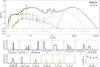 |
Fig. 2 Top panel: best-fitting model for the SED of NGC 23 (constant SFH, see Sect. 5.1) in a solid black line, together with the observed data (red diamonds). The Hα luminosity and model prediction in L⊙ units are plotted at λ = 6563 Å (red diamond and solid black circle, respectively) multiplied by a factor of 103. The solid color lines indicate the contribution of the different stellar populations with ages <10 Myr (blue), 10−100 Myr (dark green), 100–500 Myr (light green), 0.5–1.5 Gyr (orange), and > 1.5 Gyr (pink). The blue and red dashed lines are the dust emission for dust temperatures lower and higher than 50 K, respectively. The dotted green line is the AGN torus model derived by Alonso-Herrero et al. (2012a). The residuals are shown in the lower part of the panel. Bottom panels: likelihood distribution for several of the physical parameters (IR dust luminosity, SFR, stellar mass, ISM extinction μτv, young stars extinction τv, ratio between the ISM and young stars extinctions μ, fraction of IR luminosity produced by cold dust with T< 50 K removing the AGN contribution fμ, fraction of IR luminosity due to PAH emission, and dust mass). The next five panels show the logarithm of the percentage of the stellar mass for different stellar age ranges using the same color coding as in the top panel. The last panel represents the SFH. |
4.1. Stellar emission
We modeled the stellar emission by combining the emission of single stellar population bursts of different ages weighted by the stellar mass of each age. The input stellar spectra are from the POPSTAR2 library (Mollá et al. 2009; Martín-Manjón et al. 2010). Specifically, we used only those models created with the Kroupa (2001) initial mass function (IMF) and solar metallicity.
In this library there is a large number of models (106) for different stellar ages but many of them have very similar photometric colors. Because of this, we selected a set of four representative spectra of several age ranges (10−100 Myr, 100−500 Myr, 0.5−1.5 Gyr, and >1.5 Gyr; stars younger than 10 Myr are considered below through a recent star-formation burst, see below). We chose these age ranges because the variation in the mass-to-luminosity ratio is lower than a factor of two, and they have similar photometric colors, so age variations within these ranges would be almost indistinguishable using photometric information alone. We compared the POPSTAR models with the Maraston (2005) models, which include a detailed treatment of the thermally pulsing asymptotic giant branch (TP-AGB). The main differences appear in the near-IR range for populations with 0.5−1.5 Gyr, although the differences in luminosity are small, a factor of 2−3.
To combine the single stellar population models, we considered that a random fraction of the stellar mass was formed at a constant rate during the five age intervals mentioned above. We also added to the SFH a recent burst of star formation that began between 1 and 300 Myr ago (tSB) and continues until today with a constant intensity ISB between 0.03 and 10 000 times the average previous SFR.
Then, we extinguished the combined stellar spectrum following the prescription given by
Charlot & Fall (2000) and used by da Cunha et al. (2008) in the original magphys
code. That is, we assumed that stars younger than 10 Myr are still embedded in their
birth clouds (BC) and have higher extinctions than older stars, which are only affected by
the interstellar medium (ISM) extinction. Thus, for a given wavelength, the total
effective absorption, τλ, is
 for stars younger than 10 Myr and
 for older stars. For the wavelength
dependence of τλ, we used the
power-law dependence assumed by Charlot & Fall
(2000). Similar to da Cunha et al. (2008),
the input parameters regarding the extinction are τv and
μ, where
τv3
is the total extinction affecting young stars, and
for older stars. For the wavelength
dependence of τλ, we used the
power-law dependence assumed by Charlot & Fall
(2000). Similar to da Cunha et al. (2008),
the input parameters regarding the extinction are τv and
μ, where
τv3
is the total extinction affecting young stars, and  . We also computed the amount of energy
that is absorbed by dust (Ldust) and the fraction of this absorbed
energy that is produced by stars older than 10 Myr (fμ). These two parameters
are used later in Sect. 4.4 to combine the stellar
models with the IR emission models.
. We also computed the amount of energy
that is absorbed by dust (Ldust) and the fraction of this absorbed
energy that is produced by stars older than 10 Myr (fμ). These two parameters
are used later in Sect. 4.4 to combine the stellar
models with the IR emission models.
The luminosities of the hydrogen recombination lines were calculated from the number of ionizing photons in the unextinguished stellar spectrum using the case B Storey & Hummer (1995) recombination coefficients. These emission lines are affected by the BC and/or the ISM extinctions as well. In total we generated 50 000 different models, which is enough to produce smooth likelihood distributions in the fits.
4.2. IR emission
For the IR emission we used a two-component model: dust thermal emission and polycyclic
aromatic hydrocarbon (PAH) emission. For the former component we assumed that the
temperature distribution of the dust mass follows a power law, dMd/ dT ∝
T− γ with a low
temperature cut-off, Tmin (see, e.g., Dale et al. 2001; Kovács et al.
2010). We assumed that the dust emission for a given temperature is a graybody
with fixed β =
2 and an absorption coefficient κ = 0.517 m2 kg-1 at 240 μm (Li & Draine 2001). We estimated the fraction of the IR luminosity
produced by dust with T<
50 K ( ) to separate the fraction of the IR
luminosity that is produced in photodissociation regions (PDR, U ~ 2004) and that produced in more diffuse regions (Draine & Li 2007).
) to separate the fraction of the IR
luminosity that is produced in photodissociation regions (PDR, U ~ 2004) and that produced in more diffuse regions (Draine & Li 2007).
The PAH emission consists of several emission bands in the mid-IR range between 3 and 20 μm. To obtain a “pure” PAH template we used the Smith et al. (2007) average 5–35 μm mid-IR spectra of local star-forming galaxies after subtracting the underlying hot dust continuum using the pahfit code (Smith et al. 2007). We added the PAH feature at 3.3 μm using a Drude profile with an intensity equal to one third of the 6.2 μm PAH feature (Draine & Li 2007).
The dust emission model and the PAH template were combined into the final model assuming that the PAH luminosity can represent between 1 and 40% of the total IR luminosity. We produced 20 000 IR emission models with random values for γ, Tmin, and PAH luminosity fractions (qPAH).
4.3. AGN contribution
Most of the galaxies in our sample are part of the larger sample of LIRGs studied by Alonso-Herrero et al. (2012a). In that work the AGN contribution to the mid-IR emission was estimated decomposing their 5–38 μm Spitzer low-resolution spectra using star-formation templates (Brandl et al. 2006; Rieke et al. 2009) and clumpy torus models (Nenkova et al. 2008). Although, in general, the AGN energy outputin the IR is small compared to that of star formation in these galaxies (see Table 1), at certain wavelengths the AGN contribution can be noticeable. For this reason we used the torus model fitted by Alonso-Herrero et al. (2012a), when an AGN was detected, to subtract the AGN IR emission from our integrated measurements.
Only for CGCG 468-002 NED01 and NGC 7770 does the AGN dominate the mid-IR emission.
4.4. Bayesian parameter inference
To determine the likelihood distributions of the physical parameters, we modified the
magphys code so we could make use of the models we constructed. First, stellar
and IR models are combined to obtain the complete SED requiring that
 . In total, we find about 470 million
combinations that fulfill this requirement. Then, the SED models are scaled to match the
observed photometric fluxes and Hα emission. A probability (e− χ2/
2) is assigned to each model by considering upper limits when
present in the SED (see Appendix B). Finally, the
likelihood distributions of the parameters are derived from these probabilities (see da Cunha et al. 2008, for details).
. In total, we find about 470 million
combinations that fulfill this requirement. Then, the SED models are scaled to match the
observed photometric fluxes and Hα emission. A probability (e− χ2/
2) is assigned to each model by considering upper limits when
present in the SED (see Appendix B). Finally, the
likelihood distributions of the parameters are derived from these probabilities (see da Cunha et al. 2008, for details).
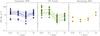 |
Fig. 4 Star-formation histories derived from the SED fitting. In the left panel we show the SFH of those galaxies with a constant SFH in blue. In the central panel, we plot those SFH with a recent burst of SF (green). In the right panel we show those SFH with a decaying SFR (orange). |
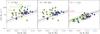 |
Fig. 5 SFR vs. stellar masses at three different age intervals calculated from the SFH. The color of the symbols is as in Fig. 4. The solid and dashed black lines are the M-S relation and uncertainty, respectively, derived by Elbaz et al. (2007) for SDSS galaxies at z ~ 0. The horizontal dashed red line marks the approximate threshold SFR needed to reach a log LIR/L⊙> 11 (excluding the AGN luminosity) based on our calibration (Sect. 5.2). Galaxies below the LIRG threshold are close companions of the sources identified as LIRGs using low angular resolution (2′) IRAS data (see Sect. 2). |
4.5. Fitting results
To fit the SED of our sample of LIRGs (Tables 5 and 6), we used the procedure described in the previous section. For most of these integrated measurements, the statistical error is low (< 5%) so most of the uncertainty comes from systematic errors, such as the absolute flux calibration, the uncertain aperture correction for semi-extended sources, and possible aperture mismatches. Therefore, we assumed a conservative 20% systematic error for all the photometric points in our SED added in quadrature to the, typically very low, statistical error.
In Figs. 2 and 3 we show the results of SED fitting for two of our galaxies: one with a constant SFH and the other with a strong burst of recent SF (see Sect. 5.1). For the rest of the sample, they are shown in Appendix D. The fitted parameters are listed in Table 7.
The best-fitting model for each galaxy is able to closely reproduce the observed SED for most of the galaxies except for IC 860 and Zw 049-057. Their optical g and r emissions are clearly underestimated by the best-fitting models (see Appendix D). This can be caused by the presence of a deeply obscured energy source (AGN or SF), which is only detected through its far-IR emission or an extinction behavior that is more complex than the one assumed in the models. In either case, the derived parameters may be uncertain, so we decided to exclude them from the discussion of Sects. 5.1 and 5.2.
Results.
5. Results and discussion
5.1. Star-formation histories
From the Bayesian fitting of the SEDs we derived likelihood distributions for the SFH of these galaxies based on the different SFH of the models. As explained in Sect. 4.1, with the photometric information alone, we are able to distinguish stellar populations in limited age intervals. Because of this, we calculated the SFH in four intervals with the same duration in log scale (i.e., 0–10 Myr, 10−100 Myr, 0.1–1 Gyr, 1–10 Gyr). These intervals are almost exactly the same as we used to construct the SED models.
To classify these SFH we first tested whether they are compatible with a constant SFR (see Fig. 4).For 17 out of 36 galaxies, we found that their SFH deviate less than 3σ from a constant SFR during their histories (averaged over the time intervals specified above). The mean uncertainty of the SFR in each interval is ~0.5 dex, so we are not able to detect variations lower than a factor of ~3 in the SFR. These 17 galaxies are mostly spirals, some of them with clearly disturbed morphologies (e.g., NGC 1961 or NGC 5653).For two cases we found a decaying SFR, and the remaining 17 galaxies (50% of the sample) show a SFH with a SF burst in the 0–100 Myr intervals. We did not find significant differences between the SFR in the 0–10 Myr and 10−100 Myr ranges for any of the galaxies, including those with a burst of SF (starbursts in the following) and those with nearly constant SFR.
The SFH of the identified starbursts indicates that the current burst began on average between30–300 Myr ago. The upper limit of this range is calculated by estimating how long it would be possible to sustain the burst intensity during the 0.1−1 Gyr interval and still detect a relative SF burst in the 10−100 Myr interval. Similarly, the lower limit is calculated by doing the same for the 1–10 Myr and 10−100 Myr intervals. This burst duration is similar to the one derived by Marcillac et al. (2006), 40–260 Myr from the modeling of Balmer absorption lines and the 4000 Å break in z = 0.7 LIRGs. The intensity of the current burst is between 2 and 20 times with a median of 7.5 times the previous averaged SFR (Table 8).
Galaxies with the higher burst intensities(> 10) are those whose morphologies are highly disturbed, indicating
recent or ongoing interactions (MCG +12-02-001, NGC 1614, CGCG 468-002 NED02, Arp 299, and
NGC 6052). However, in our sample there is one object (MCG –02-33-098) that is also an
interacting system with two nuclei separated by ~4 kpc, but its burst intensity is
only(2.5 ). Combining the age of the burst with its
intensity, we calculate the stellar mass produced by the current burst of SF with respect
to the current stellar mass (Table 8), which can be
>10−30% in these mergers. For the rest of the
galaxies, the mass formed tends to be <10%, although there is a continuous distribution of formed mass
fractions between the extreme bursts of mergers and the weaker SF bursts of other galaxies
in our sample.
). Combining the age of the burst with its
intensity, we calculate the stellar mass produced by the current burst of SF with respect
to the current stellar mass (Table 8), which can be
>10−30% in these mergers. For the rest of the
galaxies, the mass formed tends to be <10%, although there is a continuous distribution of formed mass
fractions between the extreme bursts of mergers and the weaker SF bursts of other galaxies
in our sample.
Star-formation burst properties
In Fig. 5 we plot the SFR averaged over the 0−10 Myr, 10−100 Myr, and 0.1−1 Gyr intervals vs. the stellar mass today, 100 Myr ago, and 1 Gyr ago. From the lefthand panel of this figure, it is clear that those galaxies classified as starbursts lie above the SFR-M⋆ main-sequence (M-S), as expected, while those with a relatively constant SFH are consistent with the M-S relation within 2σ.
Figure 5 shows the luminosity threshold for a galaxy to be classified as LIRG (log LIR/L⊙> 11). According to this luminosity criterion,there are eight starbursts and five M-S galaxies with LIRG luminosities due to star formation in our sample. The latter set of galaxies(NGC 23, NGC 877, NGC 1961, NGC 2388, and NGC 7771) are spirals classified as LIRGs, although they do not have a particularly high specific SFR(sSFR = SFR/M⋆< 0.4 Gyr-1). They lie within 1σ in the M-S, and since they are relatively massice (log M⋆/M⊙> 11.0), their expected SFR imply IR luminosities above or close to the LIRG luminosity threshold.
The starburst LIRGs have enhanced SFR with respect to the M-S, with the most extreme cases(Arp 299, NGC 6052, MCG +12-02-001, and NGC 1614) being mergers with high specific sSFR> 1.0 Gyr-1 (see Table 7). The rest of starbursts includespiral galaxies with different degrees of disturbed morphologies (e.g., NGC 6701 and NGC 5936). The AGN contribution to the IR luminosities is small in our sample (Table 1and Alonso-Herrero et al. 2012a), therefore the presence of an AGNdoes not affect their classification as LIRGs.
Both the lefthand and middle panels of Fig. 5 show similar distributions of the galaxies in the M⋆-SFR plane. As indicated before, this is probably because the star-formation bursts have been active during the past ~100 Myr. However, in the righthand panel (0.1–1 Gyr range; z ~ 0.075), the situation is completely different. Almost all the galaxies are in agreement with the M-S relation, and only one or two objects, with log M⋆/M⊙> 11.1, would have been classified as LIRGs if they had been observed ~1 Gyr ago.
5.1.1. Comparison with previous results for local U/LIRGs
Rodríguez Zaurín et al. (2009, 2010) used optical spectroscopy to study the SFH of local ULIRGs and find that young stellar populations (age < 100 Myr) usually dominate the stellar mass of these systems. Most of their ULIRGs are mergers in different evolutionary stages, so we compare their results with the five mergers in our sample with burst intensities > 10. In our merger LIRGs, the stellar mass formed during the ongoing burst is up to ~30%, slightly lower than in ULIRGs, although they are also compatible with burst stellar mass fractions as low as 5−10% (see Table 8).
Rodríguez Zaurín et al. (2009) argue that an old stellar population (> 2 Gyr) is not present in most of the optical spectra of ULIRGs, which is consistent with the best-fitting models for our merger LIRGs (Fig. 3 and Appendix D) where the optical light is dominated by young stars (10−100 Myr). Similar results regarding the stellar masses of ULIRGs were obtained by da Cunha et al. (2010) using magphys. In that study they also found that the median dust mass in their ULIRGs is 108.6M⊙, which is almost a factor of 10 higher than the dust masses derived for these LIRGs. However, the dust mass determination in ULIRGs is uncertain because it is not easy to constrain the cold dust temperature, which contributes significantly to the dust mass but not to the IR luminosity (da Cunha et al. 2010). Actually, they obtain a median fμ of 0.1, while fμ ranges between 0.6 and 0.9 in our sample, indicating that, in contrast to ULIRGs, dust with T< 50 K dominates the IR SEDs of LIRGs.
The resolved stellar populations of local LIRGs were examined by Alonso-Herrero et al. (2010) for nine objects in our sample using optical integral field spectroscopy. These nine objects are mostly spirals or weakly interacting galaxies. They found a higher contribution of old stellar populations to the total stellar mass in these LIRGs than in ULIRGs. This agrees with our result of lower mass fractions formed during the current burst of SF in spiral-like LIRGs than in merging LIRGs.
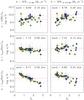 |
Fig. 6 IR and Hα luminosity/SFR ratio as a function of the fitted total extinction, Av considering the 1−10 and 10−100 Myr to average the SFR. The median ratio (solid red line) and the scatter (dashed red line) are indicated in each plot. The contribution of the AGN torus has been subtracted when present. The color of the symbols is as in Fig. 4. |
5.2. Hα vs. IR luminosity. Tracing the last 100 Myr SFH
Hα and IR luminosities are two fundamental SFR tracers. The former traces the most recent SFR since its luminosity is proportional to the number of ionizing photons, although it is necessary to apply an extinction correction that is not always accurately known. The latter, however, traces the obscured SFR, and it is virtually unaffected by foreground extinction, although it depends on the extinction level in the star-forming regions (e.g., objects with no extinction do not emit in the IR; Kennicutt & Evans 2012).
Figure 6 shows that our calibrations between the IR luminosity and the SFR at 1–10 Myr and 10−100 Myr, both ~(9.64 ± 0.18) L⊙/(M⊙ yr-1), are in very good agreement with the Kennicutt (1998) calibration of 9.57 L⊙/(M⊙ yr-1) (after correcting for the different IMF assumed). We also show in this figure the relation between the extinction-corrected Hα luminosities derived from the SED analysis with the SFR. The log Lcorr(Hα)/SFR ratio is (7.14 ± 0.09) L⊙/(M⊙ yr-1), so similar, although slightly lower than the calibration given by Kennicutt (1998) for the Hα luminosity, 7.33 L⊙/(M⊙ yr-1).
In the same way, we obtained the SFR calibration for the uncorrected Hα luminosity. The correlation between the Lobs(Hα)/SFR ratio and the extinction (Av) is clear. However, since the average integrated extinction of these LIRGs is not extremely high, τv = 0.5−3 or Av = 0.6 − 3.3 mag (see also Alonso-Herrero et al. 2006), the observed Hα luminosity could be used to estimate the integrated SFR in similar galaxies within a factor of ~3.
We find that both the LIR /SFR and the Lcorr(Hα)/SFR ratios are approximately constant and do not clearly depend on the age interval used to average the SFR. However, part of the scatter of these relations can be explained by the differences in the SFH and the extinction level. This is clearer in Fig. 7 where we plot the LIR /Lcorr(Hα) ratio as a function of the extinction comparing the observed galaxies and our models predictions. We expect this ratio to depend mainly on the relative intensities of the current SF and the average SFR during the last 100 Myr because Hα emission is only produced by young stars, whereas older stars contribute to the IR luminosity, too. But this ratio also depends on the extinction because the fraction of absorbed photons later re-emitted in the IR increases with the extinction. The latter effect is apparent in this figure since the LIR /Lcorr(Hα) ratio increases, with Av tending asymptotically to the ratio expected when 100% of the stellar light is absorbed and re-emitted by dust.
In our sample, the age effect is more subtle because, according to the derived SFH, the SFR during the last 100 Myr has been approximately constant (see Sect. 5.1). In any case, to test this dependence we computed the expected LIR /Lcorr(Hα) ratio as a function of the extinction for several log SFR1−10 Myr/SFR10 − 100 Myr ratios. The model ratios are plotted in Fig. 7, and we can see that our sample of LIRGs is, as expected, in agreement with the ratios for nearly constant SFH in the last 100 Myr. However, it should be noted that this ratio shows a strong dependence on the SFH.
For comparison, the empirical relation between the corrected Hα luminosity and a linear combination of the observed Hα luminosity and the IR luminosity derived by Kennicutt et al. (2009) for a sample of nearby galaxies is plotted in Fig. 7. The agreement between the data, our models with log SFR1−10 Myr/SFR10 − 100 Myr = 0−1, and the Kennicutt et al. (2009) relation is good within the uncertainties. This comparison suggests that the empirical relation is only valid for galaxies with constant or nearly constant SFH during the last 100 Myr. Likewise, this diagram can be readily used to distinguish between galaxies with approximately constant SFH, such as those in the M-S and galaxies with a recent (less than 100 Myr old) SF burst that would lie below the Kennicutt et al. (2009) relation.
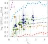 |
Fig. 7 LIR/corrected Hα luminosity ratio as a function of the total extinction, Av. The dashed lines represent the expected ratio derived from our models for various log SFR1 − 10 Myr/SFR10 − 100 Myr values (red = 2, orange = 1, turquoise = 0, blue = –1, and purple = –2). The dot-dashed black line is the ratio calculated from empirical relation Lcorr(Hα) = Lobs(Hα) + 0.0024 LIR derived by Kennicutt et al. (2009) for a sample of nearby galaxies, and the dotted black lines are the uncertainty of that calibration. The contribution of the AGN torus to the IR luminosity has been subtracted when present. The color of the symbols is as in Fig. 4. |
6. Summary and conclusions
We modeled the integrated SED of a sample of 38 local IR bright sources with IR luminosities ranging from log LIR/L⊙ = 10.2 to 11.8 and a median of log LIR/L⊙ = 11.0 belonging to 29 systems with log LIR/L⊙ = 11.0 − 11.8. The SEDs include new optical g, r, and Hα narrow-band imaging obtained with the NOT telescope combined with archival observations from UV to far-IR. To fit the SED, we modified the Bayesian code magphys (da Cunha et al. 2008) and created a set of stellar population synthesis models and dust models optimized for these objects. This SED fitting approach takes the balance into account between the energy absorbed in the UV/optical spectral ranges and that re-emitted in the IR. Except for three LIRGs that might host a deeply obscured energy source (AGN or SF), the SED models are able to reproduce the observed data well. The main results are summarized in the following:
-
1.
We classified the galaxies of our sample in three groups according to their SFH:objects with a recent burst of SF (47%), objects with a constant SFH (47%), and objects with decaying SFR (6%). In all cases the averaged SFR during the last 100 Myr seems to be relatively constant within a factor of three.
-
2.
The intensity of the recent SF burst with respect to the previous averaged SFR varies between a factor of 2 and 20, and it began~30–300 Myr ago. The most extreme bursts(intensities >10) are associated with mergers and high sSFR (>0.8 Gyr-1). Similar to local ULIRGs, these objects would be compatible with a large part (up to 30%) of their current stellar mass being formed during the ongoing SF burst event. The rest of the stabursts include galaxies with varied morphologies: mergers, disturbed spirals, interacting pairs, and isolated disks.
-
3.
Galaxies with constant SFH in our sample tend to be more massive than those with a burst of SF (median log M⋆/M⊙ = 11.0 vs. 10.6). Most of them lie just slightly above (<2σ) the M-S of galaxies, but they reach the LIRG luminosity threshold thanks to their high stellar masses.
-
4.
The calculated SFHs of the galaxies in our sample reveal that all of them had SFR and stellar masses in very good agreement with local M-S ~ 1 Gyr ago (z ~ 0.075). Their stellar masses were between 109.7 and 1011.4 M⊙ and their SFR between 0.5 and 20 M⊙ yr-1. It is likely that only one or two of them would have been classified as LIRGs if they would had observed 1 Gyr ago.
-
5.
We find that the L(IR)/Lcorr(Hα) vs. integrated optical extinction (Av) relation derived for our galaxies is in good agreement with the empirical correlation of Kennicutt et al. (2009). Our models show that this relation holds only if the SFR has been approximately constant during the last 100 Myr. Deviations from this relation can be used to identify galaxies with rapidly changing (increasing or decreasing) SFR during the last 100 Myr period.
Similar studies covering wider IR luminosity ranges and including integrated spectroscopic information will be crucial for obtaining a more detailed evolutionary history of local U/LIRGs, as well as for studying the differences and similarities with their high-z counterparts.
Online material
Appendix A: Optical spectra of nine galaxies
 |
Fig. A.1 Nuclear optical spectra of nine galaxies of our sample obtained with the FAST Spectrograph in the ranges 480–510 Å and 637–680 Å. The dashed lines mark the position of the Hβ, [O iii]λ5007 Å, Hα, and [N ii]λ6584 Å transitions. |
We present the optical spectra of nine galaxies in our sample without a previously published [N ii]/Hα ratio, to best of our knowledge. Their reduced spectra were available through the Smithsonian Astrophysical Observatory Telescope Data Center. They were obtained between 1998 and 2006 with the FAST Spectrograph (Tokarz & Roll 1997) on the Mount Hopkins Tillinghast 1.5 m reflector. The slit width was 3′′ and the spectra cover the spectral range between 3700 and 7500 Å with a dispersion of 1.5 Å per pixel. The integration times were between 600 and 1500 s. The spectra are not flux-calibrated, but they can be used to measure line ratios between transitions close in wavelength.
In the spectra shown in FigureA.1, we measured the fluxes of the Hβ, [O iii]λ5007 Å, Hα, and [N ii]λ6584 Å emission lines using a single-component Gaussian fit, except for CGCG 468-002 NED01, which shows a blue-shifted broad Hα component. The FWHM of the narrow component in this galaxy is ~500 km s-1 (Alonso-Herrero et al. 2013), whereas the broad Hα component has a FWHM of 3100 ± 190 km s-1 and is blue-shifted by 180 ± 60 km s-1. The observed line ratios are listed in Table A.1. Hβ is not corrected for stellar absorption.
We used the standard optical diagnostic diagram [N ii]/Hα vs. [O iii]/Hβ (Baldwin et al. 1981) to determine the nuclear activity classification. We used the boundary limits between H ii, composite and AGN galaxies proposed by Kewley et al. (2006). Figure A.2 shows that four of the galaxies lie in the composite region of the diagram, one in the H ii region, although close to the H ii-composite border, and one galaxy, CGCG 468-002 NED01, is classified as AGN. Since in this object we only detect a broad component in Hα, we classify it as Sy1.9. For UGC 03405 and NGC 7753, the Hβ and [O iii]λ5007 Å transitions were not detected so we excluded these objects from the diagram. However, the high [N ii]/Hα ratio in these two sources, together with the absence of [O iii] detections, which is bright in AGNs, suggests that these are composite galaxies.
Optical line ratios and nuclear activity classification.
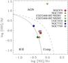 |
Fig. A.2 [N ii]λ6584 Å/Hα vs. [O iii]λ5007 Å/Hβ diagnostic diagram for the nuclear spectra of six LIRGs. The solid and dashed black lines mark the empirical separation between H ii, composite, and AGN galaxies from Kewley et al. (2006). |
Appendix B: Likelihood with detections and upper limits
In this appendix we briefly describe how the upper limits are included in our Bayesian analysis (see, e.g., Gregory 2005; Bohm & Zech 2010, for a general description of the Bayesian approach). We let Fi and σi be the flux and 1σ uncertainty
measured for a galaxy in the band i. If the galaxy is not detected, we measure the
nσi
upper limit. Likewise, the prediction of the model k for the flux of band
i is
Mi(k).
The likelihood is defined as 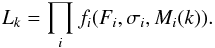 (B.1)For the detections we assume that
fi follows a normal
distribution
(B.1)For the detections we assume that
fi follows a normal
distribution ![\appendix \setcounter{section}{2} \begin{equation} f^d_i(F_i, \sigma_i, M_i) = \frac{1}{\sqrt{2 \pi \sigma_i}} \exp \left[-\frac{\left( F_i - M_i\right)^2}{2\sigma_i^2} \right] \cdot \end{equation}](/articles/aa/full_html/2015/05/aa25359-14/aa25359-14-eq275.png) (B.2)On the other hand, to obtain the likelihood
for the upper limits,
(B.2)On the other hand, to obtain the likelihood
for the upper limits,  , we first calculate the probability for
the flux to have an arbitrary value Ri. The unknown
background in the aperture used to measure the flux is Bi. The standard
deviation of the background is σi, and for
simplicity we assume that the mean background of the image is zero. That the galaxy flux
is Ri but we do not
detect it on the image at a nσi
level is because Ri +
Bi<nσi.
If the background follows a normal distribution the probability of this is
, we first calculate the probability for
the flux to have an arbitrary value Ri. The unknown
background in the aperture used to measure the flux is Bi. The standard
deviation of the background is σi, and for
simplicity we assume that the mean background of the image is zero. That the galaxy flux
is Ri but we do not
detect it on the image at a nσi
level is because Ri +
Bi<nσi.
If the background follows a normal distribution the probability of this is 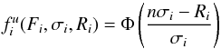 (B.3)where Φ is the cumulative distribution function
of the standard normal distribution. Therefore the likelihood value for the upper limits
is
(B.3)where Φ is the cumulative distribution function
of the standard normal distribution. Therefore the likelihood value for the upper limits
is ![\appendix \setcounter{section}{2} \begin{equation} \label{eqn:upper} f_i^u(F_i, \sigma_i, R_i) = \frac{1}{2}\left[1 + {\rm erf}\left(\frac{n\sigma_i - R_i}{\sigma_i\sqrt{2}}\right) \right] \cdot \end{equation}](/articles/aa/full_html/2015/05/aa25359-14/aa25359-14-eq282.png) (B.4)Then when substituting Eqs. (B.3) and (B.4) into Eq. (B.1),
(B.4)Then when substituting Eqs. (B.3) and (B.4) into Eq. (B.1),
![\appendix \setcounter{section}{2} \begin{eqnarray} \label{eqn:like1} L_k &=& \prod_{i_1} \frac{1}{\sqrt{2 \pi \sigma_{i_1}}} \exp \left[-\frac{\left( F_{i_1} - M_{i_1}(k)\right)^2}{2\sigma_{i_1}^2} \right] \\ \nonumber &&\quad\times \prod_{i_2} \frac{1}{2}\left[1 + {\rm erf}\left(\frac{n\sigma_{i_2} - M_{i_2}(k)}{\sigma_{i_2}\sqrt{2}}\right) \right] \end{eqnarray}](/articles/aa/full_html/2015/05/aa25359-14/aa25359-14-eq283.png) (B.5)where i1 and
i2 are the subindices for the detections
and non-detections, respectively. The logarithm of Eq. (B.5) is
(B.5)where i1 and
i2 are the subindices for the detections
and non-detections, respectively. The logarithm of Eq. (B.5) is ![\appendix \setcounter{section}{2} \begin{eqnarray} \ln L_k &=& \sum_{i_1} -\frac{\left( F_{i_1} - M_{i_1}(k)\right)^2}{2\sigma_{i_1}^2} \\ \nonumber && \quad+ \sum_{i_2} \ln \left[1 + {\rm erf}\left(\frac{n\sigma_{i_2} - M_{i_2}(k)}{\sigma_{i_2}\sqrt{2}}\right) \right] + C\\ \nonumber &=& -\frac{1}{2} \chi^2_k + \sum_{i_2} \ln \left[1 + {\rm erf}\left(\frac{n\sigma_{i_2} - M_{i_2}(k)}{\sigma_{i_2}\sqrt{2}}\right) \right] + C. \end{eqnarray}](/articles/aa/full_html/2015/05/aa25359-14/aa25359-14-eq286.png) (B.6)Thus, we assign the following probability
to model k
in the parameter inference process
(B.6)Thus, we assign the following probability
to model k
in the parameter inference process
![\appendix \setcounter{section}{2} \begin{equation} L_k = \exp \left(-\frac{1}{2} \chi^2_k \right) \prod_{i_2} \left[1 + {\rm erf}\left(\frac{n\sigma_{i_2} - M_{i_2}(k)}{\sigma_{i_2}\sqrt{2}}\right) \right] \cdot \end{equation}](/articles/aa/full_html/2015/05/aa25359-14/aa25359-14-eq287.png) (B.7)
(B.7)
Appendix C: Multi-wavelength imaging of the LIRGs
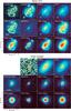 |
Fig. C.1 continued. |
 |
Fig. C.1 continued. |
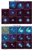 |
Fig. C.1 continued. |
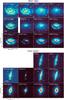 |
Fig. C.1 continued. |
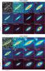 |
Fig. C.1 continued. |
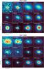 |
Fig. C.1 continued. |
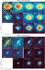 |
Fig. C.1 continued. |
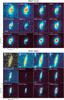 |
Fig. C.1 continued. |
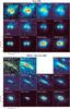 |
Fig. C.1 continued. |
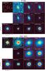 |
Fig. C.1 continued. |
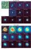 |
Fig. C.1 continued. |
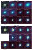 |
Fig. C.1 continued. |
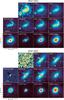 |
Fig. C.1 continued. |
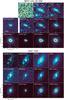 |
Fig. C.1 continued. |
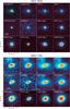 |
Fig. C.1 continued. |
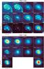 |
Fig. C.1 continued. |
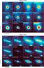 |
Fig. C.1 continued. |
Appendix D: Best fitting model results to the SED
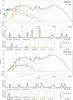 |
Fig. D.1 continued. |
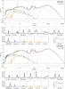 |
Fig. D.1 continued. |
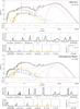 |
Fig. D.1 continued. |
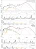 |
Fig. D.1 continued. |
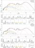 |
Fig. D.1 continued. |
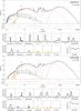 |
Fig. D.1 continued. |
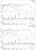 |
Fig. D.1 continued. |
 |
Fig. D.1 continued. |
 |
Fig. D.1 continued. |
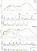 |
Fig. D.1 continued. |
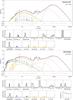 |
Fig. D.1 continued. |
 |
Fig. D.1 continued. |
 |
Fig. D.1 continued. |
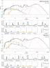 |
Fig. D.1 continued. |
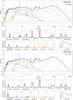 |
Fig. D.1 continued. |
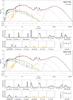 |
Fig. D.1 continued. |
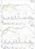 |
Fig. D.1 continued. |
Two or more lines of the Baldwin et al. (1981) diagrams were not detected in their optical spectra.
Acknowledgments
We thank the anonymous referee for comments and suggestions.We also thank the Nordic Optical Telescope and Isaac Newton Group staff for their support during the observations. We acknowledge support from the Spanish Plan Nacional de Astronomía y Astrofísica through grants AYA2010-21161-C02-1, AYA2010-21887-C04-03, AYA2012-32295, AYA2012-31447, AYA2012-31277, and AYA2012-39408-C02-01. Based on observations made with the Nordic Optical Telescope, operated by the Nordic Optical Telescope Scientific Association at the Observatorio del Roque de los Muchachos, La Palma, Spain, of the Instituto de Astrofisica de Canarias. The data presented here were obtained in part with ALFOSC, which is provided by the Instituto de Astrofisica de Andalucia (IAA) under a joint agreement with the University of Copenhagen and NOTSA. This research has made use of the NASA/IPAC Extragalactic Database (NED) which is operated by the Jet Propulsion Laboratory, California Institute of Technology, under contract with the National Aeronautics and Space Administration.
References
- Aihara, H., Allen de Prieto, C., An, D., et al. 2011, ApJS, 193, 29 [NASA ADS] [CrossRef] [Google Scholar]
- Alonso-Herrero, A., Rieke, G. H., Rieke, M. J., et al. 2006, ApJ, 650, 835 [NASA ADS] [CrossRef] [Google Scholar]
- Alonso-Herrero, A., García-Marín, M., Monreal-Ibero, A., et al. 2009, A&A, 506, 1541 [NASA ADS] [CrossRef] [EDP Sciences] [Google Scholar]
- Alonso-Herrero, A., García-Marín, M., Rodríguez Zaurín, J., et al. 2010, A&A, 522, A7 [NASA ADS] [CrossRef] [EDP Sciences] [Google Scholar]
- Alonso-Herrero, A., Pereira-Santaella, M., Rieke, G. H., & Rigopoulou, D. 2012a, ApJ, 744, 2 [NASA ADS] [CrossRef] [Google Scholar]
- Alonso-Herrero, A., Rosales-Ortega, F. F., Sánchez, S. F., et al. 2012b, MNRAS, 425, L46 [NASA ADS] [CrossRef] [Google Scholar]
- Alonso-Herrero, A., Pereira-Santaella, M., Rieke, G. H., et al. 2013, ApJ, 765, 78 [Google Scholar]
- Arribas, S., Bushouse, H., Lucas, R. A., Colina, L., & Borne, K. D. 2004, AJ, 127, 2522 [NASA ADS] [CrossRef] [Google Scholar]
- Baan, W. A., Salzer, J. J., & Lewinter, R. D. 1998, ApJ, 509, 633 [NASA ADS] [CrossRef] [Google Scholar]
- Baldwin, J. A., Phillips, M. M., & Terlevich, R. 1981, PASP, 93, 5 [NASA ADS] [CrossRef] [EDP Sciences] [Google Scholar]
- Bohm, G., & Zech, G. 2010, Introduction to Statistics and Data Analysis for Physicists (Verlag Deutsches Elektronen-Synchrotron) [Google Scholar]
- Bournaud, F., Jog, C. J., & Combes, F. 2007, A&A, 476, 1179 [NASA ADS] [CrossRef] [EDP Sciences] [Google Scholar]
- Brandl, B. R., Bernard-Salas, J., Spoon, H. W. W., et al. 2006, ApJ, 653, 1129 [NASA ADS] [CrossRef] [Google Scholar]
- Brown, M. J. I., Moustakas, J., Smith, J.-D. T., et al. 2014, ApJS, 212, 18 [Google Scholar]
- Calzetti, D., Wu, S.-Y., Hong, S., et al. 2010, ApJ, 714, 1256 [NASA ADS] [CrossRef] [Google Scholar]
- Caputi, K. I., Lagache, G., Yan, L., et al. 2007, ApJ, 660, 97 [NASA ADS] [CrossRef] [Google Scholar]
- Charlot, S., & Fall, S. M. 2000, ApJ, 539, 718 [NASA ADS] [CrossRef] [Google Scholar]
- da Cunha, E., Charlot, S., & Elbaz, D. 2008, MNRAS, 388, 1595 [NASA ADS] [CrossRef] [Google Scholar]
- da Cunha, E., Charmandaris, V., Díaz-Santos, T., et al. 2010, A&A, 523, A78 [NASA ADS] [CrossRef] [EDP Sciences] [Google Scholar]
- Dale, D. A., Helou, G., Contursi, A., Silbermann, N. A., & Kolhatkar, S. 2001, ApJ, 549, 215 [NASA ADS] [CrossRef] [Google Scholar]
- Draine, B. T., & Li, A. 2007, ApJ, 657, 810 [NASA ADS] [CrossRef] [Google Scholar]
- Elbaz, D., Daddi, E., Le Borgne, D., et al. 2007, A&A, 468, 33 [NASA ADS] [CrossRef] [EDP Sciences] [Google Scholar]
- Farrah, D., Bernard-Salas, J., Spoon, H. W. W., et al. 2007, ApJ, 667, 149 [NASA ADS] [CrossRef] [Google Scholar]
- Farrah, D., Lonsdale, C. J., Weedman, D. W., et al. 2008, ApJ, 677, 957 [NASA ADS] [CrossRef] [Google Scholar]
- Fazio, G. G., Hora, J. L., Allen, L. E., et al. 2004, ApJS, 154, 10 [NASA ADS] [CrossRef] [Google Scholar]
- Fitzpatrick, E. L. 1999, PASP, 111, 63 [NASA ADS] [CrossRef] [Google Scholar]
- García-Marín, M., Colina, L., Arribas, S., Alonso-Herrero, A., & Mediavilla, E. 2006, ApJ, 650, 850 [NASA ADS] [CrossRef] [Google Scholar]
- Gregory, P. C. 2005, Bayesian Logical Data Analysis for the Physical Sciences (Cambridge University Press) [Google Scholar]
- Griffin, M. J., Abergel, A., Abreu, A., et al. 2010, A&A, 518, L3 [Google Scholar]
- Hammer, F., Flores, H., Elbaz, D., et al. 2005, A&A, 430, 115 [NASA ADS] [CrossRef] [EDP Sciences] [Google Scholar]
- Ho, L. C., Filippenko, A. V., & Sargent, W. L. W. 1997, ApJS, 112, 315 [NASA ADS] [CrossRef] [Google Scholar]
- Hung, C.-L., Sanders, D. B., Casey, C. M., et al. 2014, ApJ, 791, 63 [Google Scholar]
- Jarrett, T. H., Chester, T., Cutri, R., et al. 2000, AJ, 119, 2498 [NASA ADS] [CrossRef] [Google Scholar]
- Jarrett, T. H., Chester, T., Cutri, R., Schneider, S. E., & Huchra, J. P. 2003, AJ, 125, 525 [NASA ADS] [CrossRef] [Google Scholar]
- Kartaltepe, J. S., Sanders, D. B., Le Floc’h, E., et al. 2010, ApJ, 721, 98 [NASA ADS] [CrossRef] [Google Scholar]
- Keel, W. C. 1984, ApJ, 282, 75 [NASA ADS] [CrossRef] [Google Scholar]
- Kennicutt, Jr., R. C. 1998, ARA&A, 36, 189 [Google Scholar]
- Kennicutt, R. C., & Evans, N. J. 2012, ARA&A, 50, 531 [NASA ADS] [CrossRef] [Google Scholar]
- Kennicutt, Jr., R. C., & Kent, S. M. 1983, AJ, 88, 1094 [NASA ADS] [CrossRef] [Google Scholar]
- Kennicutt, R. C., Hao, C., Calzetti, D., et al. 2009, ApJ, 703, 1672 [NASA ADS] [CrossRef] [Google Scholar]
- Kewley, L. J., Heisler, C. A., Dopita, M. A., & Lumsden, S. 2001, ApJS, 132, 37 [NASA ADS] [CrossRef] [Google Scholar]
- Kewley, L. J., Groves, B., Kauffmann, G., & Heckman, T. 2006, MNRAS, 372, 961 [NASA ADS] [CrossRef] [Google Scholar]
- Kovács, A., Omont, A., Beelen, A., et al. 2010, ApJ, 717, 29 [NASA ADS] [CrossRef] [Google Scholar]
- Kroupa, P. 2001, MNRAS, 322, 231 [NASA ADS] [CrossRef] [Google Scholar]
- Lasker, B. M., Lattanzi, M. G., McLean, B. J., et al. 2008, AJ, 136, 735 [NASA ADS] [CrossRef] [PubMed] [Google Scholar]
- Le Floc’h, E., Papovich, C., Dole, H., et al. 2005, ApJ, 632, 169 [NASA ADS] [CrossRef] [Google Scholar]
- Li, A., & Draine, B. T. 2001, ApJ, 554, 778 [Google Scholar]
- Maraston, C. 2005, MNRAS, 362, 799 [NASA ADS] [CrossRef] [Google Scholar]
- Marcillac, D., Elbaz, D., Charlot, S., et al. 2006, A&A, 458, 369 [NASA ADS] [CrossRef] [EDP Sciences] [Google Scholar]
- Martin, D. C., Fanson, J., Schiminovich, D., et al. 2005, ApJ, 619, L1 [Google Scholar]
- Martín-Manjón, M. L., García-Vargas, M. L., Mollá, M., & Díaz, A. I. 2010, MNRAS, 403, 2012 [NASA ADS] [CrossRef] [Google Scholar]
- Masetti, N., Bassani, L., Bazzano, A., et al. 2006, A&A, 455, 11 [NASA ADS] [CrossRef] [EDP Sciences] [Google Scholar]
- Mollá, M., García-Vargas, M. L., & Bressan, A. 2009, MNRAS, 398, 451 [NASA ADS] [CrossRef] [Google Scholar]
- Moustakas, J., & Kennicutt, Jr., R. C. 2006, ApJS, 164, 81 [NASA ADS] [CrossRef] [Google Scholar]
- Nardini, E., Risaliti, G., Salvati, M., et al. 2009, MNRAS, 399, 1373 [NASA ADS] [CrossRef] [Google Scholar]
- Nenkova, M., Sirocky, M. M., Nikutta, R., Ivezić, Ž., & Elitzur, M. 2008, ApJ, 685, 160 [NASA ADS] [CrossRef] [Google Scholar]
- Noll, S., Burgarella, D., Giovannoli, E., et al. 2009, A&A, 507, 1793 [NASA ADS] [CrossRef] [EDP Sciences] [Google Scholar]
- Pereira-Santaella, M., Alonso-Herrero, A., Santos-Lleo, M., et al. 2011, A&A, 535, A93 [NASA ADS] [CrossRef] [EDP Sciences] [Google Scholar]
- Pérez-González, P. G., Rieke, G. H., Egami, E., et al. 2005,ApJ, 630, 82 [Google Scholar]
- Petric, A. O., Armus, L., Howell, J., et al. 2011, ApJ, 730, 28 [NASA ADS] [CrossRef] [Google Scholar]
- Pilbratt, G. L., Riedinger, J. R., Passvogel, T., et al. 2010, A&A, 518, L1 [CrossRef] [EDP Sciences] [Google Scholar]
- Poglitsch, A., Waelkens, C., Geis, N., et al. 2010, A&A, 518, L2 [NASA ADS] [CrossRef] [EDP Sciences] [Google Scholar]
- Rieke, G. H., Young, E. T., Engelbracht, C. W., et al. 2004, ApJS, 154, 25 [NASA ADS] [CrossRef] [Google Scholar]
- Rieke, G. H., Alonso-Herrero, A., Weiner, B. J., et al. 2009, ApJ, 692, 556 [NASA ADS] [CrossRef] [Google Scholar]
- Rigby, J. R., Marcillac, D., Egami, E., et al. 2008, ApJ, 675, 262 [NASA ADS] [CrossRef] [Google Scholar]
- Rodríguez Zaurín, J., Tadhunter, C. N., & González Delgado, R. M. 2009, MNRAS, 400, 1139 [NASA ADS] [CrossRef] [Google Scholar]
- Rodríguez Zaurín, J., Tadhunter, C. N., & González Delgado, R. M. 2010, MNRAS, 403, 1317 [NASA ADS] [CrossRef] [Google Scholar]
- Roussel, H. 2013, PASP, 125, 1126 [Google Scholar]
- Sanders, D. B., & Mirabel, I. F. 1996, ARA&A, 34, 749 [NASA ADS] [CrossRef] [Google Scholar]
- Sanders, D. B., Mazzarella, J. M., Kim, D.-C., Surace, J. A., & Soifer, B. T. 2003, AJ, 126, 1607 [Google Scholar]
- Skibba, R. A., Engelbracht, C. W., Dale, D., et al. 2011, ApJ, 738, 89 [NASA ADS] [CrossRef] [Google Scholar]
- Skrutskie, M. F., Cutri, R. M., Stiening, R., et al. 2006, AJ, 131, 1163 [NASA ADS] [CrossRef] [Google Scholar]
- Smith, J. A., Tucker, D. L., Kent, S., et al. 2002, AJ, 123, 2121 [Google Scholar]
- Smith, J. D. T., Draine, B. T., Dale, D. A., et al. 2007, ApJ, 656, 770 [NASA ADS] [CrossRef] [Google Scholar]
- Storey, P. J., & Hummer, D. G. 1995, MNRAS, 272, 41 [NASA ADS] [CrossRef] [Google Scholar]
- Surace, J. A., Sanders, D. B., & Mazzarella, J. M. 2004, AJ, 127, 3235 [NASA ADS] [CrossRef] [Google Scholar]
- Tokarz, S. P., & Roll, J. 1997, in Astronomical Data Analysis Software and Systems VI, eds. G. Hunt, & H. Payne, ASP Conf. Ser., 125, 140 [Google Scholar]
- Tueller, J., Mushotzky, R. F., Barthelmy, S., et al. 2008, ApJ, 681, 113 [NASA ADS] [CrossRef] [Google Scholar]
- U, V., Sanders, D. B., Mazzarella, J. M., et al. 2012, ApJS, 203, 9 [NASA ADS] [CrossRef] [Google Scholar]
- Veilleux, S., Kim, D.-C., Sanders, D. B., Mazzarella, J. M., & Soifer, B. T. 1995, ApJS, 98, 171 [NASA ADS] [CrossRef] [Google Scholar]
- Veilleux, S., Kim, D., & Sanders, D. B. 2002, ApJS, 143, 315 [NASA ADS] [CrossRef] [Google Scholar]
- Werner, M. W., Roellig, T. L., Low, F. J., et al. 2004, ApJS, 154, 1 [Google Scholar]
- Yuan, T.-T., Kewley, L. J., & Sanders, D. B. 2010, ApJ, 709, 884 [NASA ADS] [CrossRef] [Google Scholar]
All Tables
All Figures
|
Fig. 1 Subset of the images used to construct the integrated SED of NGC 23. The new NOT optical observations of the g, r, and Hα+[N ii] bands are shown. The rest of the images were obtained from the public archives of their respective observatories (see Sect. 3 for details). Some images used in the SED are not displayed here because they have morphologies similar to those of the presented images (2MASS J and H, IRAC 4.5 and 5.8 μm, and PACS 100 μm) or because they have a very low angular resolution (SPIRE 350 and 500 μm). All images are shown in a logarithm scale. North is up and east to the left. The white bar in the Hα+[N ii] panel represents 10 kpc at the distance of the object. |
| In the text | |
|
Fig. 2 Top panel: best-fitting model for the SED of NGC 23 (constant SFH, see Sect. 5.1) in a solid black line, together with the observed data (red diamonds). The Hα luminosity and model prediction in L⊙ units are plotted at λ = 6563 Å (red diamond and solid black circle, respectively) multiplied by a factor of 103. The solid color lines indicate the contribution of the different stellar populations with ages <10 Myr (blue), 10−100 Myr (dark green), 100–500 Myr (light green), 0.5–1.5 Gyr (orange), and > 1.5 Gyr (pink). The blue and red dashed lines are the dust emission for dust temperatures lower and higher than 50 K, respectively. The dotted green line is the AGN torus model derived by Alonso-Herrero et al. (2012a). The residuals are shown in the lower part of the panel. Bottom panels: likelihood distribution for several of the physical parameters (IR dust luminosity, SFR, stellar mass, ISM extinction μτv, young stars extinction τv, ratio between the ISM and young stars extinctions μ, fraction of IR luminosity produced by cold dust with T< 50 K removing the AGN contribution fμ, fraction of IR luminosity due to PAH emission, and dust mass). The next five panels show the logarithm of the percentage of the stellar mass for different stellar age ranges using the same color coding as in the top panel. The last panel represents the SFH. |
| In the text | |
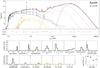 |
Fig. 3 Same as Fig. 2 but for Arp 299 (recent SF burst, see Sect. 5.1). |
| In the text | |
|
Fig. 4 Star-formation histories derived from the SED fitting. In the left panel we show the SFH of those galaxies with a constant SFH in blue. In the central panel, we plot those SFH with a recent burst of SF (green). In the right panel we show those SFH with a decaying SFR (orange). |
| In the text | |
|
Fig. 5 SFR vs. stellar masses at three different age intervals calculated from the SFH. The color of the symbols is as in Fig. 4. The solid and dashed black lines are the M-S relation and uncertainty, respectively, derived by Elbaz et al. (2007) for SDSS galaxies at z ~ 0. The horizontal dashed red line marks the approximate threshold SFR needed to reach a log LIR/L⊙> 11 (excluding the AGN luminosity) based on our calibration (Sect. 5.2). Galaxies below the LIRG threshold are close companions of the sources identified as LIRGs using low angular resolution (2′) IRAS data (see Sect. 2). |
| In the text | |
|
Fig. 6 IR and Hα luminosity/SFR ratio as a function of the fitted total extinction, Av considering the 1−10 and 10−100 Myr to average the SFR. The median ratio (solid red line) and the scatter (dashed red line) are indicated in each plot. The contribution of the AGN torus has been subtracted when present. The color of the symbols is as in Fig. 4. |
| In the text | |
|
Fig. 7 LIR/corrected Hα luminosity ratio as a function of the total extinction, Av. The dashed lines represent the expected ratio derived from our models for various log SFR1 − 10 Myr/SFR10 − 100 Myr values (red = 2, orange = 1, turquoise = 0, blue = –1, and purple = –2). The dot-dashed black line is the ratio calculated from empirical relation Lcorr(Hα) = Lobs(Hα) + 0.0024 LIR derived by Kennicutt et al. (2009) for a sample of nearby galaxies, and the dotted black lines are the uncertainty of that calibration. The contribution of the AGN torus to the IR luminosity has been subtracted when present. The color of the symbols is as in Fig. 4. |
| In the text | |
|
Fig. A.1 Nuclear optical spectra of nine galaxies of our sample obtained with the FAST Spectrograph in the ranges 480–510 Å and 637–680 Å. The dashed lines mark the position of the Hβ, [O iii]λ5007 Å, Hα, and [N ii]λ6584 Å transitions. |
| In the text | |
|
Fig. A.2 [N ii]λ6584 Å/Hα vs. [O iii]λ5007 Å/Hβ diagnostic diagram for the nuclear spectra of six LIRGs. The solid and dashed black lines mark the empirical separation between H ii, composite, and AGN galaxies from Kewley et al. (2006). |
| In the text | |
 |
Fig. C.1 Same as Fig. 1. |
| In the text | |
|
Fig. C.1 continued. |
| In the text | |
|
Fig. C.1 continued. |
| In the text | |
|
Fig. C.1 continued. |
| In the text | |
|
Fig. C.1 continued. |
| In the text | |
|
Fig. C.1 continued. |
| In the text | |
|
Fig. C.1 continued. |
| In the text | |
|
Fig. C.1 continued. |
| In the text | |
|
Fig. C.1 continued. |
| In the text | |
|
Fig. C.1 continued. |
| In the text | |
|
Fig. C.1 continued. |
| In the text | |
|
Fig. C.1 continued. |
| In the text | |
|
Fig. C.1 continued. |
| In the text | |
|
Fig. C.1 continued. |
| In the text | |
|
Fig. C.1 continued. |
| In the text | |
|
Fig. C.1 continued. |
| In the text | |
|
Fig. C.1 continued. |
| In the text | |
|
Fig. C.1 continued. |
| In the text | |
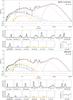 |
Fig. D.1 Same as Fig. 2. |
| In the text | |
|
Fig. D.1 continued. |
| In the text | |
|
Fig. D.1 continued. |
| In the text | |
|
Fig. D.1 continued. |
| In the text | |
|
Fig. D.1 continued. |
| In the text | |
|
Fig. D.1 continued. |
| In the text | |
|
Fig. D.1 continued. |
| In the text | |
|
Fig. D.1 continued. |
| In the text | |
|
Fig. D.1 continued. |
| In the text | |
|
Fig. D.1 continued. |
| In the text | |
|
Fig. D.1 continued. |
| In the text | |
|
Fig. D.1 continued. |
| In the text | |
|
Fig. D.1 continued. |
| In the text | |
|
Fig. D.1 continued. |
| In the text | |
|
Fig. D.1 continued. |
| In the text | |
|
Fig. D.1 continued. |
| In the text | |
|
Fig. D.1 continued. |
| In the text | |
|
Fig. D.1 continued. |
| In the text | |
Current usage metrics show cumulative count of Article Views (full-text article views including HTML views, PDF and ePub downloads, according to the available data) and Abstracts Views on Vision4Press platform.
Data correspond to usage on the plateform after 2015. The current usage metrics is available 48-96 hours after online publication and is updated daily on week days.
Initial download of the metrics may take a while.