| Issue |
A&A
Volume 577, May 2015
|
|
|---|---|---|
| Article Number | A78 | |
| Number of page(s) | 53 | |
| Section | Extragalactic astronomy | |
| DOI | https://doi.org/10.1051/0004-6361/201425359 | |
| Published online | 06 May 2015 | |
Online material
Appendix A: Optical spectra of nine galaxies
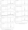 |
Fig. A.1
Nuclear optical spectra of nine galaxies of our sample obtained with the FAST Spectrograph in the ranges 480–510 Å and 637–680 Å. The dashed lines mark the position of the Hβ, [O iii]λ5007 Å, Hα, and [N ii]λ6584 Å transitions. |
| Open with DEXTER | |
We present the optical spectra of nine galaxies in our sample without a previously published [N ii]/Hα ratio, to best of our knowledge. Their reduced spectra were available through the Smithsonian Astrophysical Observatory Telescope Data Center. They were obtained between 1998 and 2006 with the FAST Spectrograph (Tokarz & Roll 1997) on the Mount Hopkins Tillinghast 1.5 m reflector. The slit width was 3′′ and the spectra cover the spectral range between 3700 and 7500 Å with a dispersion of 1.5 Å per pixel. The integration times were between 600 and 1500 s. The spectra are not flux-calibrated, but they can be used to measure line ratios between transitions close in wavelength.
In the spectra shown in FigureA.1, we measured the fluxes of the Hβ, [O iii]λ5007 Å, Hα, and [N ii]λ6584 Å emission lines using a single-component Gaussian fit, except for CGCG 468-002 NED01, which shows a blue-shifted broad Hα component. The FWHM of the narrow component in this galaxy is ~500 km s-1 (Alonso-Herrero et al. 2013), whereas the broad Hα component has a FWHM of 3100 ± 190 km s-1 and is blue-shifted by 180 ± 60 km s-1. The observed line ratios are listed in Table A.1. Hβ is not corrected for stellar absorption.
We used the standard optical diagnostic diagram [N ii]/Hα vs. [O iii]/Hβ (Baldwin et al. 1981) to determine the nuclear activity classification. We used the boundary limits between H ii, composite and AGN galaxies proposed by Kewley et al. (2006). Figure A.2 shows that four of the galaxies lie in the composite region of the diagram, one in the H ii region, although close to the H ii-composite border, and one galaxy, CGCG 468-002 NED01, is classified as AGN. Since in this object we only detect a broad component in Hα, we classify it as Sy1.9. For UGC 03405 and NGC 7753, the Hβ and [O iii]λ5007 Å transitions were not detected so we excluded these objects from the diagram. However, the high [N ii]/Hα ratio in these two sources, together with the absence of [O iii] detections, which is bright in AGNs, suggests that these are composite galaxies.
Optical line ratios and nuclear activity classification.
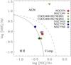 |
Fig. A.2
[N ii]λ6584 Å/Hα vs. [O iii]λ5007 Å/Hβ diagnostic diagram for the nuclear spectra of six LIRGs. The solid and dashed black lines mark the empirical separation between H ii, composite, and AGN galaxies from Kewley et al. (2006). |
| Open with DEXTER | |
Appendix B: Likelihood with detections and upper limits
In this appendix we briefly describe how the upper limits are included in our Bayesian analysis (see, e.g., Gregory 2005; Bohm & Zech 2010, for a general description of the Bayesian approach). We let Fi and σi be the flux and 1σ uncertainty
measured for a galaxy in the band i. If the galaxy is not detected, we measure the
nσi
upper limit. Likewise, the prediction of the model k for the flux of band
i is
Mi(k).
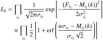
The likelihood is defined as ![]() (B.1)For the detections we assume that
fi follows a normal
distribution
(B.1)For the detections we assume that
fi follows a normal
distribution  (B.2)On the other hand, to obtain the likelihood
for the upper limits,
(B.2)On the other hand, to obtain the likelihood
for the upper limits, ![]() , we first calculate the probability for
the flux to have an arbitrary value Ri. The unknown
background in the aperture used to measure the flux is Bi. The standard
deviation of the background is σi, and for
simplicity we assume that the mean background of the image is zero. That the galaxy flux
is Ri but we do not
detect it on the image at a nσi
level is because Ri +
Bi<nσi.
If the background follows a normal distribution the probability of this is
, we first calculate the probability for
the flux to have an arbitrary value Ri. The unknown
background in the aperture used to measure the flux is Bi. The standard
deviation of the background is σi, and for
simplicity we assume that the mean background of the image is zero. That the galaxy flux
is Ri but we do not
detect it on the image at a nσi
level is because Ri +
Bi<nσi.
If the background follows a normal distribution the probability of this is 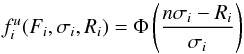 (B.3)where Φ is the cumulative distribution function
of the standard normal distribution. Therefore the likelihood value for the upper limits
is
(B.3)where Φ is the cumulative distribution function
of the standard normal distribution. Therefore the likelihood value for the upper limits
is 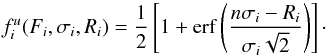 (B.4)Then when substituting Eqs. (B.3) and (B.4) into Eq. (B.1),
 (B.5)where i1 and
i2 are the subindices for the detections
and non-detections, respectively. The logarithm of Eq. (B.5) is
(B.5)where i1 and
i2 are the subindices for the detections
and non-detections, respectively. The logarithm of Eq. (B.5) is 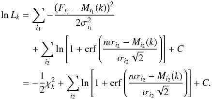 (B.6)Thus, we assign the following probability
to model k
in the parameter inference process
(B.6)Thus, we assign the following probability
to model k
in the parameter inference process
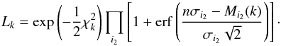 (B.7)
(B.7)
Appendix C: Multi-wavelength imaging of the LIRGs
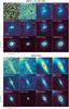 |
Fig. C.1
Same as Fig. 1. |
| Open with DEXTER | |
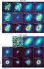 |
Fig. C.1
continued. |
| Open with DEXTER | |
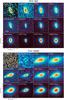 |
Fig. C.1
continued. |
| Open with DEXTER | |
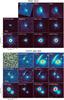 |
Fig. C.1
continued. |
| Open with DEXTER | |
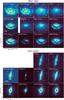 |
Fig. C.1
continued. |
| Open with DEXTER | |
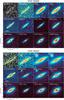 |
Fig. C.1
continued. |
| Open with DEXTER | |
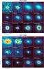 |
Fig. C.1
continued. |
| Open with DEXTER | |
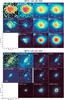 |
Fig. C.1
continued. |
| Open with DEXTER | |
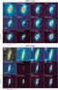 |
Fig. C.1
continued. |
| Open with DEXTER | |
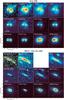 |
Fig. C.1
continued. |
| Open with DEXTER | |
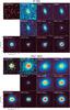 |
Fig. C.1
continued. |
| Open with DEXTER | |
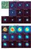 |
Fig. C.1
continued. |
| Open with DEXTER | |
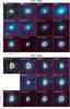 |
Fig. C.1
continued. |
| Open with DEXTER | |
 |
Fig. C.1
continued. |
| Open with DEXTER | |
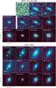 |
Fig. C.1
continued. |
| Open with DEXTER | |
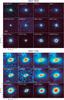 |
Fig. C.1
continued. |
| Open with DEXTER | |
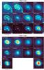 |
Fig. C.1
continued. |
| Open with DEXTER | |
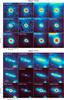 |
Fig. C.1
continued. |
| Open with DEXTER | |
Appendix D: Best fitting model results to the SED
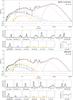 |
Fig. D.1
Same as Fig. 2. |
| Open with DEXTER | |
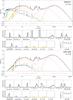 |
Fig. D.1
continued. |
| Open with DEXTER | |
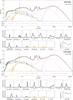 |
Fig. D.1
continued. |
| Open with DEXTER | |
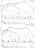 |
Fig. D.1
continued. |
| Open with DEXTER | |
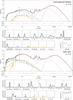 |
Fig. D.1
continued. |
| Open with DEXTER | |
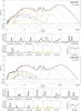 |
Fig. D.1
continued. |
| Open with DEXTER | |
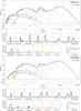 |
Fig. D.1
continued. |
| Open with DEXTER | |
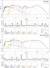 |
Fig. D.1
continued. |
| Open with DEXTER | |
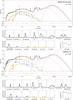 |
Fig. D.1
continued. |
| Open with DEXTER | |
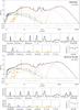 |
Fig. D.1
continued. |
| Open with DEXTER | |
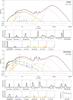 |
Fig. D.1
continued. |
| Open with DEXTER | |
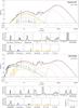 |
Fig. D.1
continued. |
| Open with DEXTER | |
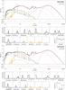 |
Fig. D.1
continued. |
| Open with DEXTER | |
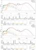 |
Fig. D.1
continued. |
| Open with DEXTER | |
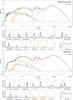 |
Fig. D.1
continued. |
| Open with DEXTER | |
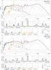 |
Fig. D.1
continued. |
| Open with DEXTER | |
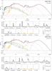 |
Fig. D.1
continued. |
| Open with DEXTER | |
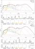 |
Fig. D.1
continued. |
| Open with DEXTER | |
© ESO, 2015
Current usage metrics show cumulative count of Article Views (full-text article views including HTML views, PDF and ePub downloads, according to the available data) and Abstracts Views on Vision4Press platform.
Data correspond to usage on the plateform after 2015. The current usage metrics is available 48-96 hours after online publication and is updated daily on week days.
Initial download of the metrics may take a while.