A thin diffuse component of the Galactic ridge X-ray emission and heating of the interstellar medium contributed by the radiation of Galactic X-ray binaries

Margherita Molaro; Rishi Khatri; Rashid A. Sunyaev

doi:10.1051/0004-6361/201323332

Home

All issues

Volume 564 (April 2014)

A&A, 564 (2014) A107

Full HTML

Free Access

Issue		A&A Volume 564, April 2014


Article Number		A107
Number of page(s)		24
Section		Interstellar and circumstellar matter
DOI		https://doi.org/10.1051/0004-6361/201323332
Published online		16 April 2014

A&A 564, A107 (2014)

A thin diffuse component of the Galactic ridge X-ray emission and heating of the interstellar medium contributed by the radiation of Galactic X-ray binaries^⋆

Margherita Molaro¹, Rishi Khatri¹ and Rashid A. Sunyaev¹^,2

¹ Max Planck Institut für Astrophysik, Karl-Schwarzschild-Str. 1, 85741 Garching, Germany
e-mail: molaro@mpa-garching.mpg.de
² Space Research Institute, Russian Academy of Sciences, Profsoyuznaya 84/32, 117997 Moscow, Russia

Received: 23 December 2013
Accepted: 14 January 2014

Abstract

We predict a thin diffuse component of the Galactic ridge X-ray emission (GRXE) arising from the scattering of the radiation of bright X-ray binaries (XBs) by the interstellar medium. This scattered component has the same scale height as that of the gaseous disk (~80 pc) and is therefore thinner than the GRXE of stellar origin (scale height ~130 pc). The morphology of the scattered component is furthermore expected to trace the clumpy molecular and HI clouds. We calculate this contribution to the GRXE from known Galactic XBs assuming that they are all persistent. The known XBs sample is incomplete, however, because it is flux limited and spans the lifetime of X-ray astronomy (~50 years), which is very short compared with the characteristic time of 1000−10 000 years that would have contributed to the diffuse emission observed today due to time delays. We therefore also use a simulated sample of sources, to estimate the diffuse emission we should expect in an optimistic case assuming that the X-ray luminosity of our Galaxy is on average similar to that of other galaxies. In the calculations we also take into account the enhancement of the total scattering cross-section due to coherence effects in the elastic scattering from multi-electron atoms and molecules. This scattered emission can be distinguished from the contribution of low X-ray luminosity stars by the presence of narrow fluorescent K-α lines of Fe, Si, and other abundant elements present in the interstellar medium and by directly resolving the contribution of low X-ray luminosity stars. We find that within 1° latitude of the Galactic plane the scattered emission contributes on average 10 − 30% of the GRXE flux in the case of known sources and over 50% in the case of simulated sources. In the latter case, the scattered component is found to even dominate the stellar emission in certain parts of the Galactic plane. X-rays with energies ≳1 keV from XBs should also penetrate deep inside the HI and molecular clouds, where they are absorbed and heat the interstellar medium. We find that this heating rate dominates the heating by cosmic rays (assuming a solar neighborhood energy density) in a considerable part of the Galaxy.

Key words: scattering / X-rays: binaries / X-rays: ISM / X-rays: general / atomic processes / X-rays: stars

^⋆

Appendices are available in electronic form at http://www.aanda.org

© ESO, 2014

1. Introduction

The unresolved or apparently diffuse X-ray sky is composed of an isotropic component originating in extragalactic sources such as active galactic nuclei, the cosmic X-ray background (CXB) (Giacconi et al. 1962), and a component confined mostly to the plane of our Galaxy known as the Galactic ridge X-ray emission (GRXE) (Worrall et al. 1982). The latter presents prominent emission lines at 6−7 keV, which if produced by highly ionized elements in a thermal plasma would imply a temperature of 5−10 keV (Koyama et al. 1986, 1989; Tanaka 2002; Muno et al. 2004; Revnivtsev 2003). A plasma with such a high temperature could not be gravitationally bound and remain confined to the Galactic plane (Koyama et al. 1986; Sunyaev et al. 1993; Tanaka et al. 1999; Tanaka 2002), suggesting that the GRXE cannot be truly diffuse. One solution that has been explored is for the GRXE to be composed of unresolved stellar sources with low X-ray luminosity. Evidence of this includes the correlation of the emission with the stellar bulge and disk (Yamauchi & Koyama 1993; Revnivtsev 2003; Revnivtsev et al. 2006), the resolution of over 80% of the emission in a small region of the sky (Revnivtsev et al. 2009), and the similarity of the GRXE spectrum with the one produced by the superposition of the spectra of the low X-ray luminosity sources expected to contribute to the emission (Ebisawa et al. 2001, 2005; Revnivtsev et al. 2006; Morihana et al. 2013). The nature of the GRXE is, however, still not conclusively resolved.

Sunyaev et al. (1993) suggested that a part of the GRXE may arise from diffuse gas and be composed of radiation from the compact X-ray sources scattered by the interstellar medium (ISM). This component of the GRXE would also have a K-α line from neutral iron in the ISM.Koyama et al. (1996), using observations from ASCA, first resolved what was initially thought to be a 6.7 keV iron K-α line from the Galactic center into a 7 keV and 6.7 keV lines from highly ionized H-like and He-like iron, respectively, and a 6.4 keV line from neutral iron, supporting the prediction of Sunyaev et al. (1993). This was later confirmed using Suzaku observations by Koyama et al. (2007) and Ebisawa et al. (2008).

Our Galaxy is sprinkled with X-ray sources such as low-mass and high-mass binaries (LMXBs and HMXBs), supernova remnants, pulsars, and recurring novae. The X-ray radiation from these sources is scattered by free electrons, atomic and molecular hydrogen, helium, and heavier elements present in the interstellar medium. This reprocessed radiation would be seen by us as a truly diffuse component emission, approximately tracing the gas distribution in the Galaxy. This scattering of X-rays by interstellar gas is different from the dust halos seen around many X-ray sources (Overbeck 1965; Trümper & Schönfelder 1973; Rolf 1983; Predehl & Schmitt 1995). Scattering by dust decreases very sharply (approximately Gaussian) with the angle of scattering and is strong only within 1° of the source (Mauche & Gorenstein 1986; Smith & Dwek 1998). Scattering by atoms and molecules on the other hand is effective on large angles and would contribute up to 180°.

2. Expected contribution of scattered X-rays to GRXE

There have been a number of attempts to test the hypothesis that the GRXE is composed of discrete low-luminosity stellar sources (Ebisawa et al. 2001; Muno et al. 2004; Ebisawa et al. 2005; Revnivtsev et al. 2006, 2009; Morihana et al. 2013) using Chandra and X-ray Multi-Mirror Mission (XMM-Newton) observatories. Revnivtsev et al. (2009) succeeded in resolving ~80% of the emission in a narrow band around 6.7 keV into point sources in a small region of the sky of 16 × 16 arcmin centered at l = 0.08°,b = −1.42°. The resolution of the GRXE into point sources in the Galactic plane has proven more difficult because of the difficulty in separating out extragalactic sources and insufficient sensitivity and angular resolution to resolve the weak but densely populated Galactic sources. Indirect evidence that weak X-ray sources such as cataclysmic variables and coronally active binaries form a significant component of GRXE came from correlating the GRXE with the near-infrared Galactic emission, expected in this case since these sources trace the old stellar population. Revnivtsev et al. (2006) used data from the Rossi X-Ray Timing Explorer – Proportional Counter Array (RXTE/PCA) to show that the 3−20 keV component of the emission traces the stellar mass distribution and is well fitted by models of the Galactic stellar bar and disk from Dwek et al. (1995), Bahcall & Soneira (1980), Kent et al. (1991), Freudenreich (1996), and Dehnen & Binney (1998). Using results from Sazonov et al. (2006), Revnivtsev et al. (2006) also found that the GRXE broad-band spectrum is very similar to the superposition of the spectra of low-luminosity X-ray sources in the solar neighborhood. These results agree with the studies of the hard (17−60 keV) component using the IBIS telescope onboard of INTErnational Gamma-Ray Astrophysics Laboratory (INTEGRAL) by Krivonos et al. (2007a). We refer to the contribution of low luminosity (in X-rays) stellar sources to the GRXE as stellar GRXE.

This seems to suggest that the nature of the GRXE has finally been solved. However, there is still plenty of room, especially in the central degree of the Galactic plane, for a contribution from a diffuse scattered component to the GRXE, which we refer to as scattered GRXE. The scattered X-rays will follow the distribution of gas in the Galaxy with a scale height of 80 pc (0.6° at a distance of 8 kpc), in contrast to a stellar emission characterised by a scale height of 130 pc (1° at a distance of 8 kpc) (Dehnen & Binney 1998; Binney & Tremaine 2008). We therefore do not expect a significant contribution from the scattered emission in the field of view of Revnivtsev et al. (2009) at latitude b = −1.42°, but it is possible, in an optimistic model of Galactic X-ray luminosity, for the scattered component to dominate the stellar component at | b | ≲ 0.5. A significant contribution from scattered diffuse X-rays is therefore not ruled out by current observations, and it is an interesting question to ask what its contribution from scattering of luminous X-ray sources might be.

An important feature of the scattered component is that since the scattered X-rays travel a longer path to reach us from the original source, the X-rays seen by us today have contribution from the cumulative past X-ray activity of the Galaxy. This implies that even sources currently undergoing a low quiescent phase may contribute to the average X-ray Galactic output had they experienced a higher level of activity in the past. An important example is the supermassive black hole Sgr A^∗ situated at the Galactic center, which currently radiates at least eight orders of magnitude below its Eddington limit with a quiescent 2 − 10 keV luminosity of ~10³³⁻³⁴ ergs/s (e.g. Narayan et al. 1998; Baganoff et al. 2003). The scattering of the hard X-ray continuum radiation of Sgr A^∗ by an individual molecular cloud (Sgr B2) was first observed by Revnivtsev et al. (2004). Studies of the recent history of Sgr A^∗’s activity through the reflected X-rays from the massive molecular clouds in its vicinity (first proposed by Sunyaev et al. 1993; and followed by Koyama et al. 1996; Murakami et al. 2000; Revnivtsev et al. 2004; Muno et al. 2007; Inui et al. 2009; Ponti et al. 2010; Terrier et al. 2010; Capelli et al. 2012; Nobukawa et al. 2011; Gando Ryu et al. 2012; Clavel et al. 2013) suggest that the source experienced much more luminous phases in the past than currently observed (see Ponti et al. 2013, for a review). In this paper we ignore the contribution of this source and focus only on the contribution of XBs (see Appendix B for a discussion of its possible contribution compared to that of XBs).

Grimm et al. (2002) calculated the 2 − 10 keV luminosity of Galactic binary sources averaged over the period 1996-2000. They give the average luminosity of LMXBs to be 2−3 × 10³⁹ ergs/s and that of HMXBs to be 2 − 3 × 10³⁸ ergs/s from RXTE All-Sky Monitor (ASM) data. The total luminosity of the GRXE is currently estimated at ~1.39 × 10³⁸ ergs/s in the 3 − 20 keV band (Revnivtsev et al. 2006) and 3.7 ± 0.2 × 10³⁷ ergs/s in the 17 − 60 keV energy range (Krivonos et al. 2007a) with a spectrum in the 3−20 keV band with a photon index Γ ~ 1.2. For a Thomson scattering optical depth of ~1% in the ISM through the Galactic plane, we would expect the contribution to the GRXE from the scattered radiation to be ~10³⁷ ergs/s, or about 10% of the observed luminosity. In contrast to the stellar GRXE, this ~10% scattered contribution to the luminosity is concentrated in a much narrower region in the Galactic plane, giving a higher relative contribution to the local surface brightness. The sample of bright X-ray binaries we use in the calculations is incomplete, however, as is clear from a significant deficit of sources farther out than the Galactic center in the Grimm et al. (2002) sample. There is also significant uncertainty in the distances of most of the sources. Moreover, we expect many high-luminosity transients in the Galaxy with luminosities ≳10³⁸ ergs/s, which are active for only few % of the time. Such transients would contribute to the observed scattered flux today but would not be present in the current sample if they were inactive at the time of observations.

A better estimate of the average X-ray luminosity of the Milky Way is possible by considering the relation of LMXB and HMXB populations with other Galactic properties such as the stellar mass (M_⋆) and the star formation rate (SFR). The long evolutionary timescales of the low-mass donor star imply that LMXBs are expected to follow the older stellar population, while the short lifetime of the high-mass donors in HMXBs means that they should trace the younger stellar population of the Galaxy. Grimm et al. (2002) pointed out that we should therefore expect a relationship between the LMXB luminosity and M_⋆ on the one hand and between the HMXB luminosity and the SFR of a galaxy on the other. Grimm et al. (2003) and Gilfanov (2004) extended these studies to other galaxies which were followed by Ranalli et al. (2003), Colbert et al. (2004), Persic & Rephaeli (2007), Lehmer et al. (2010) and Mineo et al. (2012) and up to redshift z ~ 1.3 using 66 galaxies in Mineo et al. (2014). The study of these relations in other galaxies avoids issues of incompleteness and distance uncertainties, which are important in the study of local XBs. These studies assume a linear relationship between the total 2−10 keV luminosity $L_{X}^{2 - 10 keV}$ $\hbox{$L_{\rm X}^{2-10~{\rm keV}}$}$ of LMXBs and HMXBs and the total M_⋆ and SFR of the galaxy respectively, that is $L_{X}^{2 - 10 keV} ~ α \times M_{⋆} + β \times SFR .$ $\begin{equation} L_{\rm X}^{2-10~{\rm keV}}\sim \alpha \times M_{\star}+ \beta \times SFR.\label{lehmer} \end{equation}$ (1)Estimated values for the proportionality factors are α ~ 8 × 10²⁸ erg/(s M_⊙) (Gilfanov 2004) and β ~ 2.2 − 2.6 × 10³⁹ erg/(s M_⊙ yr^-1) (Grimm et al. 2003; Shtykovskiy & Gilfanov 2005; Lehmer et al. 2010; Mineo et al. 2012).

The Milky Way is therefore subluminous in LMXBs by a factor of ~2, consistent with the original results of Gilfanov (2004), and by a factor of ~30 in luminosity of HMXBs compared with the other galaxies. The large discrepancy for the HMXBs may be explained if we take into account that there is a delay of 10⁶−10⁷ years between the time of starburst and appearance of HMXBs (Gilfanov 2004; Shtykovskiy & Gilfanov 2007), corresponding to the evolutionary timescale of the donor star, which implies that the relevant SFR is not the present SFR, but the SFR of a million years ago. However, if we assume, optimistically for our purpose, that the discrepancy is caused by the incompleteness of the observed sample and the short lifespan of X-ray astronomy of about 50 years, it is possible that we happen to live in a time where the observed X-ray luminosity of our Galaxy is below average and that if averaged over a time-scale of 10³ − 10⁴ years our Galaxy would turn out to have an average luminosity consistent with that observed in other galaxies.

The X-ray luminosity of most galaxies including our own is dominated by a few extremely bright sources, and different sources may be the main contributors at different times. Existence in the past of a few ultra-luminous X-ray sources (ULXs) with luminosities of 10³⁹ − 10⁴⁰ erg/s, as observed in some star-forming galaxies, would significantly affect the scattered component, making it significantly brighter (Khatri & Sunyaev, in prep.). Therefore such a strong temporal fluctuation is plausible. This is also supported by the scatter of more than an order of magnitude in the luminosity-SFR relations (Mineo et al. 2014) and by the broad probability distributions for the X-ray luminosity at low star formation rates (Gilfanov et al. 2004).

For a Milky Way stellar mass of 6 × 10¹⁰ M_⊙ (McMillan 2011) and star formation rate of ~1 M_⊙/ yr (see for example Robitaille & Whitney 2010) we should expect, under this assumption and based on above studies, an average LMXB luminosity of 5 × 10³⁹ ergs/s and HMXB luminosity of 2−3 × 10³⁹ ergs/s. These estimates are higher by a factor of ~2 (for LMXBs) and a factor of ~10 (for HMXBs) than the values, respectively, quoted by Grimm et al. (2002).

In this optimistic case, we expect that in the Galactic plane almost 50% of the contribution to the GRXE might come from the scattered radiation. The observation of this thin component of the GRXE would therefore allow one to test this hypothesis.

The true luminosity probably lies somewhere between these two extremes. We consider both a Monte Carlo population of XB sources based on Eq. (1) to study the most luminous optimistic case, and a catalog of XB sources with known distances and spectral parameters from RXTE/ASM and INTEGRAL surveys to place a lower bound on the contribution of this effect.

We also take into account the coherent or Rayleigh scattering of the X-ray radiation on multi-electron species such as H2, He, and heavy elements. Rayleigh scattering significantly increases the GRXE flux especially when the scattering angles are small. This applies to the scattering from the HMXBs, which lie mostly in the plane of the Galaxy. Details of the effect of Rayleigh scattering are discussed in Appendix C. Molecular clouds are thus very important and would be detected as regions of high X-ray intensity in the GRXE. The compact nature of molecular clouds additionally boosts the scattered intensity, with molecular clouds evident as luminous features in the maps. These features are clearly seen in our maps of diffuse scattered component of the GRXE using the data from Boston University-Five College Radio Astronomy Observatory Galactic Ring Survey (Jackson et al. 2006).

The stellar component of the GRXE will also be scattered in the ISM and will form part of the scattered GRXE. We expect this component to be subdominant and to contribute only ~τ~1% to the GRXE. For completeness we explicitly calculate and include this component. The scattering of isotropic CXB, on the other hand, cannot be observed if we ignore the small change in the spectrum of X-rays due to loss of energy to electron recoil in Compton scattering and does not need to be taken into account. We therefore leave the detailed calculation of scattering of CXB on cold atomic and molecular gas for a future publication (Molaro et al., in prep.).

3. Galaxy model

The gas in the interstellar medium in the disk of the Galaxy has a multiphase character (McKee & Ostriker 1977) loosely classified into atomic (neutral or ionized) gas and molecular gas, with the atomic gas further classified into cold neutral medium (CNM), warm neutral medium (WNM), warm ionized medium (WIM) and hot ionized medium (HIM) (see Kalberla & Kerp 2009, for a recent review), while a significant part of the molecular gas is concentrated in giant molecular clouds (GMCs). Most of the mass in the neutral atomic gas is confined to the disk of the Galaxy and is clearly traced by HI 21 cm emission. The maps of the HI 21 cm emission in the Galaxy (Kalberla et al. 2005; McClure-Griffiths et al. 2009) can only provide the total column density in parts of the sky, for example toward the Galactic center, where the velocity information cannot be used to infer the three-dimensional gas distribution. The CNM, which contains most of the HI, is clumped into clouds that have a volume filling factor of ~10-20% in the plane of the Galaxy in the solar neighborhood (Kalberla & Kerp 2009). Any given line of sight should therefore intersect many clouds, making the column density much smoother. A smooth disk model therefore suffices for our calculation and we use the models of Dehnen & Binney (1998) and Binney & Tremaine (2008) for the HI gas distribution.

The situation is slightly different for molecular clouds. The GMCs, mainly concentrated near the Galactic center and in the spiral arms, have sizes of ~10 − 100 pc and average densities on the order of 10² − 10³ cm^-3 with mean separation between the clouds 10 times the mean size (Blitz 1993; McKee & Ostriker 2007), giving a volume-filling factor in the plane of the Galaxy of ~0.1%. They are therefore compact enough to significantly influence the morphology of the X-ray signal. The full-sky maps of the molecular gas distribution using CO lines (Dame et al. 2001) do not resolve and provide distances to individual clouds (Dame et al. 2001), although high-resolution studies of many important GMCs are available. Recently, high-resolution data with kinematic distances have been made available from the Boston University-Five College Radio Astronomy Observatory Galactic Ring Survey (GRS) (Jackson et al. 2006; Rathborne et al. 2009; Roman-Duval et al. 2009, 2010), which covers the very important molecular ring structure in the inner Milky Way. We use these data to predict the X-ray scattering signal in the longitude range 18° ≤ ℓ ≤ 55.7° and latitude range −1° ≤ b ≤ 1°. Although GRS covers only a 10% of the Galactic plane, the results are easily extendable to and are valid for the full sky, and in particular clearly show the spatial morphology and features in the GRXE expected from the molecular clouds.

3.1. ISM distribution

The total ISM mass in both atomic and molecular form within a Galactocentric radius R ≲ 20 kpc of the Galaxy is approximately 9.5 × 10⁹M_⊙ (Kalberla & Kerp 2009), with hydrogen (HI and H2) accounting for 71% of this mass. The ratio of average atomic to molecular gas is 4.9 within R ≲ 20 kpc (Draine 2011), giving a total HI mass of 5.6 × 10⁹M_⊙ and a total H2 mass of 1.15 × 10⁹M_⊙ within this radius. Because of the incompleteness of the GRS, we use a smooth disk model for the mass distribution of HI and H2 for full Galactic plane calculations with the above normalizations and use H2 data from the GRS (Jackson et al. 2006; Roman-Duval et al. 2009, 2010) for calculations limited to the longitude range covered by the survey. The latter case is used to study the effect of clumpiness and small volume-filling factor of the molecular clouds on the observed X-ray intensity morphology (see Sect. 5.5).

The average density distribution of the interstellar HI gas in the Galactic disk can be described by an exponential disk (Dehnen & Binney 1998; Binney & Tremaine 2008). The ISM mass density distribution at a Galactocentric distance R and Galactic plane height z used in this model is given by $ρ_{HI} (R,z) \propto \frac{1}{2 z_{d}} \exp (- \frac{R_{m}}{R} - \frac{R}{R_{d}} - \frac{| z |}{z_{d}}),$ $\begin{equation} \rho_{{\rm HI}}(R,z) \propto \frac{1}{2z_{\rm d}}{\rm exp}\left(-\frac{R_m}{R}-\frac{R}{R_{\rm d}} - \frac{|z|}{z_{\rm d}}\right), \label{Eq:diskmodel} \end{equation}$ (2)with parameters R_m = 4 kpc, R_d = 6.4 kpc and z_d = 80 pc.

The lack of HI gas in the central region of the plane, due to the central depression of radius 4 kpc in the HI disk, is compensated for by the concentration in this region of most of the H2 component, which gives a significant fraction of the scattering at low longitude values. The average H2 distribution in the Galaxy is given by Misiriotis et al. (2006) as $ρ_{H 2} (R,z) \propto \exp (- R / R_{H 2} - | z | / z_{d})$ $\begin{equation} \rho_{{\rm H2}}(R,z) \propto {\rm exp}(-R/R_{{\rm H2}}-|z|/z_d) \label{Eq:diskmodelh2} \end{equation}$ (3)with parameters R_H2 = 2.57 kpc and z_d = 80 pc as in Eq. (2).

Fig. 1

Projected distribution on the Galactic plane of persistent X-ray sources observed during the past 40 years used in our calculations, shown against the spiral structure of the Galaxy.

Fig. 2

Distribution on the sky of observed LMXBs and HMXBs sources used in the calculations for energy ranges 3−20 keV and 17−60 keV with the pointsize proportional to their luminosity in the indicated energy range. A concentration of HMXBs can be seen along the lines of sight tangential to the spiral arms.

We also account for the concentration of matter in the Galactic disk into spiral arms. This is particularly important because HMXBs are also concentrated in the Galactic spiral arms: the combined effect of concentration of HMXBs as well as atomic and molecular clouds in these structures means that we expect an enhancement of scattered X-ray intensity in the directions tangential to the spiral arms. We describe the spiral structure of the Galaxy following the prescription given in Vallee (1995), where the location of the density wave maxima of the nth spiral arm is given by $m [θ - θ_{0} - \ln (R / R_{0}) \tan (p)^{-1}] = (n - 1) 2 π,$ $\begin{equation} m\bigg[\theta - \theta_0 -{\rm ln}(R/R_0){\rm tan}(p)^{-1}\bigg] = (n-1)2\pi, \end{equation}$ (4)where m = 4 is the total number of spiral arms, p = 12° (inward) is the pitch angle and R₀ = 2.5 kpc. We have verified that the line of sights tangential to the spiral arms in the model are consistent with the location of the tangential directions based on different observations, as summarized in Vallée (2008). We model the density around the spiral maxima as a Gaussian probability distribution with respect to the projected distance from the spiral arms’ maxima on the Galactic plane d: $ρ_{Spiral} \propto \sum_{n = 1}^{m} \exp (- (d_{n} / w)^{2}),$ $\begin{equation} \rho_{\rm Spiral} \propto \sum\limits_{n=1}^m {\rm exp}(-(d_n/w)^2), \end{equation}$ (5)where the typical width w of the spiral arm is assumed to be 500 pc for the gas component. The density of the wave is assumed to be three times higher than the inter-arm density (Levine et al. 2006). The overall density distribution including the spiral structure is therefore given by $ρ_{H} (R,z,θ) \propto [1 + 3 \times ρ_{Spiral} (R,θ)^{]} ρ_{H} (R,z)$ $\begin{equation} \rho_{{\rm H}}(R,z,\theta) \propto \left[1 + 3 \times \rho_{\rm Spiral}(R,\theta)\right] \rho_{{\rm H}}(R,z) \end{equation}$ (6)for both ρ_H = ρ_HI and ρ_H = ρ_H2. The distribution of gas in the Galaxy in our model is shown in Fig. 1. We assume constant abundances for heavier elements throughout the Galaxy with abundances taken to be same as the present-day solar photosphere from Asplund et al. (2009).

3.2. Distribution of X-ray binaries in the Galaxy

Observed XBs distribution. We use time-averaged X-ray flux measurements from different surveys to compile a catalog of X-ray binary sources with known flux and position in different energy bands (2−10 keV and 17−60 keV)¹. References for distance estimates for each source are taken from the SIMBAD database.

For the energy range 17 − 60 keV we combine different INTEGRAL surveys (Krivonos et al. 2007b, 2012; Lutovinov et al. 2013) from which we select 86 LMXB and 70 HMXB Galactic sources for a total 17−60 keV luminosity of 1.97 × 10³⁸erg/s and 6.2 × 10³⁷erg/s, respectively, for which distance and best-fit spectral parameters data are available. We also consider the contribution in this range of four very luminous extragalactic HMXB sources (SMC X-1, LMC X-1, LMC X-4, IGR J05007-7047), which is, however, close to negligible.

For the lower energy range (2−10 keV) we use the list of sources given in Grimm et al. (2002)² for which distance and flux measurements from RXTE/ASM, which provides all-sky flux measurements averaged over ~5 yr, are available. We also use the relation L_{2 − 10 keV} ~ 0.5L_{17 − 60 keV} valid for NS binary sources (Filippova et al. 2005) to infer the 2−10 keV luminosity from the harder X-ray range catalog for 20 HMXB sources for which low-energy data are not available. In total, the number of sources considered in this energy range is 61 for the HMXBs, for a total 2−10 keV luminosity of 5.5 × 10³⁷ erg/s, and 81 for the LMXBs, with a total luminosity of 2.56 × 10³⁹ erg/s. The energy output of these sources in the 3−20 keV range is modeled using a model spectrum (described below for the Monte Carlo sources) with a flat intensity spectrum and an exponential cutoff at 4.6 keV and 20 keV for the LMXBs and HMXBs, respectively. In the 17−60 keV range we use the best-fit photon index from Integral surveys (Krivonos et al. 2007b) and in some cases from the literature on individual sources when the former is not available. In general, we expect variations in the photon spectrum in the 2−10 keV range from source to source and also with time. Given the uncertainties in the time-averaged spectral properties of Galactic X-ray binaries, our description of the average spectrum should be adequate. To turn the problem around, if the diffuse component of GRXE can be separated from point sources using high angular resolution observations, then the scattered GRXE measurement will directly give us the average spectrum of X-ray sources in the Galaxy, after correcting for the effect of energy dependence of Rayleigh scattering, which makes the scattered spectrum softer than the incident spectrum (see Appendix C) and the effect of X-ray absorption. The distribution of the catalog sources used in the calculations is shown in Fig. 1 as a projection on the Galactic plane and in Fig. 2 in the Galactic angular coordinates. Properties of the sources responsible for the peaks in the scattered X-ray radiation can be found in Appendix A in Table A.1.

Monte Carlo distribution.We simulate the optimistic case discussed in Sect. 2 by populating the Galaxy with a Monte Carlo simulated population of HMXBs and LMXBs. The probability density function (pdf) for the distribution of LMXBs in the Galaxy is taken to be proportional to the mass density of stars, whereas the pdf of HMXBs is taken to be proportional the mass density of the ISM; both the stars and ISM density distributions are modelled using themass models in Dehnen & Binney (1998) and Binney & Tremaine (2008) (Eq. (2)) with stellar disk parameters z_d = 325 pc, R_d = 2.5 kpc and R_m = 0. HMXBs are therefore expected to be concentrated in the plane of the Galaxy, a fact that becomes important when we include the Rayleigh scattering at small angles on multi-electron atoms and molecules. We populate the Galaxy with 300 LMXBs and 100 HMXBs using Monte Carlo samplingfrom these distributions,which is consistent with observations taking into account the incompleteness of catalog at the low-flux end (Ritter & Kolb 2003; Liu et al. 2007, 2006). The sources are assigned luminosities sampled randomly from the luminosity functions of Gilfanov (2004) for LMXBs and Grimm et al. (2003) for HMXBs. The total 2 − 10 keV luminosity of the Galaxy in our calculation is ~4.7 × 10³⁹ ergs/s for simulated LMXBs and ~1.7 × 10³⁹ ergs/s for simulated HMXBs, which is consistent with the expectations from observations of other galaxies (Grimm et al. 2002, 2003; Gilfanov 2004; Lehmer et al. 2010; Mineo et al. 2012, 2014). As discussed in the previous section, we use the following typical spectrum for all the sources, but differentiating between LMXBs and HMXBs by assuming a softer spectrum for LMXBs and a harder spectrum for HMXBs in the 3−20 keV range: $F (E) \propto E^{- α} e^{- \frac{E}{β}} s^{-1} {keV}^{-1},$ $\begin{equation} \label{spectrum} F(E)\propto E^{- \alpha}{\rm e}^{-\frac{E}{\beta}}\:\:\: {\rm s}^{-1}{\rm keV}^{-1}, \end{equation}$ (7)with parameters α = 1,β = 20keV for simulated HMXBs (Lutovinov et al. 2005a) and α = 1,β = 4.6keV for simulated LMXBs, which is a fit to the observed spectrum of GX 340+0 (Gilfanov et al. 2003).

4. Scattering of X-rays on atoms and molecules

4.1. Scattering cross-sections

Interaction of X-ray photons with light atoms is described by the following expression (see e.g. Eisenberger & Platzman 1970; Hubbell et al. 1975; Sunyaev & Churazov 1996; Sunyaev et al. 1999, for detailed discussion): $\frac{d σ}{dΩd ω_{2}} = \frac{r_{e}^{2}}{2} (1 + {\cos (θ)}^{2}) \frac{ω_{2}}{ω_{1}} | ⟨ f | \sum_{j} e^{i q r_{j}} | i ⟩ |^{2} \times δ (Δ E_{if} - Δ ω),$ $\begin{equation} \frac{{\rm d}\sigma}{{\rm d}\Omega {\rm d}\omega_2} = \frac{r_{\rm e}^2}{2}(1+{\cos(\theta)}^2)\frac{\omega_2}{\omega_1}|\langle f|\sum_{j} {\rm e}^{i\vec{q}\vec{r}_j} | i \rangle|^2 \times \delta(\Delta E_{if} - \Delta \omega), \end{equation}$ (8)where ω₁ and ω₂ are the photon energy before and after the scattering, ΔE_if and Δω = ω₁ − ω₂ denote the energy change in the atom or molecule and in the photon, respectively, i and f are the initial and final states of the system, q is the change in the photon momentum and r_j is the coordinate of the jth electron.

Depending on the final state of the system after the interaction, the processes are classified as Rayleigh or elastic scattering, involving a change in the direction of the incoming photon at constant frequency (i = f), Raman scattering, resulting in the excitation of the bound electron (f = excited state), and Compton scattering, resulting in the ionization of the atom or molecule (f = continuum state).

These cross-sections, which involve the scattering of radiation off electrons bound in atomic or molecular hydrogen, helium, and other heavy atoms and molecules, include additional effects compared to scattering off free electrons due to the discrete energy levels that they occupy and their distribution over momentum from quantum mechanical effects (Eisenberger & Platzman 1970; Sunyaev & Churazov 1996; Vainshtein et al. 1998). The latter in particular implies that the energy of the scattered photon is not unambiguously constrained by the scattering angle, and therefore that the Klein-Nishina (KN) formulation for the singly differential scattering cross-section is no longer sufficient. One of the most commonly used methods in computing the interaction is the impulse approximation (IA) applied to the doubly differential cross-section, which is relevant in the case of a change in the photon energy much larger than the binding energy (Eisenberger & Platzman 1970; Sunyaev & Churazov 1996). The singly differential case, on the other hand, can be computed by implementing the corrections to the KN formulation via an incoherent scattering factor S(x) (Bergstrom et al. 1993), such that ${(\frac{d σ}{dΩ} (θ))}_{Compt} = S (x (θ)) {(\frac{d σ}{dΩ} (θ))}_{KN},$ $\begin{equation} \label{comp} \left(\frac{{\rm d}\sigma}{{\rm d}\Omega} (\theta)\right)_{{\rm Compt}} = S(x(\theta)) \left(\frac{{\rm d}\sigma}{{\rm d}\Omega} (\theta)\right)_{{\rm KN}}, \end{equation}$ (9)where θ is the scattering angle and x(θ) is the momentum transfer. For heavier atoms or molecules, the most relevant differences with respect to HI scattering are found at small angles due to elastic scattering. In the presence of Z electrons in the system, these can coherently scatter the photon, enhancing the scattering at small angles, where the change in energy of the photon is weak, by a factor of Z². Furthermore, the range of angles and energies at which the elastic scattering remains dominant increases with additional electrons due to the decreasing characteristic size of the electron distribution, D. The condition that the elastic scattering dominates is in fact determined by qr_j ≲ 1, which in the small-angle approximation can be rewritten as θ2πD/λ ≲ 1, where λ is the photon’s wavelength (Sunyaev et al. 1999). The range of scattering angles over which Rayleigh scattering dominates, however, rapidly decreases with increasing energy. The enhancement of the total scattering cross-section due to coherence effects therefore mostly contributes to the scattering in the softer energy band (see Appendix C).

The computation of the elastic and inelastic cross sections for atoms is computed using the routines from the publicly available library, xraylib (Schoonjans et al. 2011), which uses results from Hubbell et al. (1975). For molecular hydrogen, which has a characteristic size of the electron distribution similar to that of HI, we approximate the scattering cross-section by including a factor Z² = 4 for elastic scattering and a factor of 2 for inelastic scattering to the HI cross section, which was shown by Sunyaev et al. (1999) to be a reasonable approximation. Heavier elements included in the calculations are chosen based on their fractional contribution to the elastic scattering cross-section. Ranking heavier elements by their maximal contribution to Rayleigh scattering (proportional to Z² × n_Z/n_H), we include contributions from He, O, Fe, C, Ne, Si, and Mg in addition to H (see Table C.1). Scattering on H2 and helium is especially important for HMXBs, whose X-rays have paths to us with small scattering angles, resulting in significant enhancement of X-ray flux than for HI. The contribution from all other elements combined would be lower than ~1%. In principle, the scattering from molecules such as CO and water would be, in addition, enhanced in the Rayleigh scattering regime because of coherent scattering from all atoms in the molecules, and should be taken into account in a precise calculation. For example, in CO the cross section in the Rayleigh limit will be 196 × Thomson in the molecule, compared with 100 × Thomson if the two atoms were separate. Given the uncertainties in the fraction of elements in molecules and the depletion of elements in dust, in addition to the uncertainties in metallicities in different regions of the Galaxy, such a precise treatment is not warranted at this stage, and we ignore these otherwise important effects.

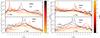Fig. 3

Profiles of the volume emissivity per deg² in our direction on the Galactic plane due to the observed sources used in our calculations, at different distances from the Galactic center (Sun’s position (−8 kpc, 0, 0.015 kpc)). Units were chosen so that if this emissivity is integrated over 1 kpc it is numerically equal to the observed flux. Proximity effects in the vicinity of sources are clearly visible. The concentration of LMXBs in the Galactic bulge results in a steady decrease in the overall profile of the volume emissivity from these sources away from the Galactic center. This is not the case for HMXBs because of their distribution along the Galactic disk. Discontinuities in the LMXBs profiles in the positive y-range are caused by temporal constraints in the illumination of its surroundings by the very bright source GRS 1915+105 (located at (− 0.27 kpc,7.83 kpc, − 27 pc)), which was not observed during 1970−1992 and is assumed to have been absent before 1992.

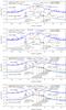Fig. 4

Longitude profiles of scattered XB radiation in comparison with a near-infrared-inferred GRXE profile in energy ranges 3−10, 10−20, 17−25, and 25−60 keV for real sources. The sum of the scattered component is 10-30% of the stellar contribution to the GRXE. Data for the sources responsible for the labeled peaks are listed in Table A.1.

4.2. ISM volume emissivity

The total volume emissivity per steradian, ϵ_XBs, of the gas due to illumination by Galactic X-ray binary sources at a distance s from the observer along the line of sight (l,b) is given by 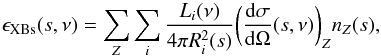$ϵ_{XBs} (s,ν) = \sum_{Z} \sum_{i} \frac{L_{i} (ν)}{4 π R_{i}^{2} (s)} (\frac{d σ}{dΩ} (s,ν))_{Z} n_{Z} (s),$ $\begin{equation} \epsilon_{{\rm XBs}} (s, \nu) = \sum_{Z} \sum_{i} \frac{L_{i}(\nu)}{4\pi R^2_i(s)} \bigg(\frac{{\rm d}\sigma}{{\rm d}\Omega}(s, \nu) \bigg )_{Z} n_{Z}(s) \label{emissivity10}, \end{equation}$ (10)where the sum is computed over the X-ray sources i and elements Z contributing to the scattering, R_i is the distance of source with luminosity L_i from the scattering point, (dσ/ dΩ) is the differential scattering cross-section including Rayleigh and Compton scattering, and n_Z is the number density distribution of the element Z. The total differential cross-section is computed as a function of the position along the line of sight s as well as of the radiation energy, since the angle at which radiation from a given source is to be scattered to reach the observer will depend on the position at which the scattering occurs. Because of the low optical depth, the contribution of radiation that undergoes multiple scatterings before reaching the observer is assumed to be negligible. The volume emissivity per unit solid angle in the Galactic plane is plotted in Fig. 3 using observed data. From Eq. (10) we expect proximity zones near individual sources where the flux peaks sharply, as clearly seen in Fig. 3. Scattering of X-rays in these proximity zones will result in X-ray halos around each source, similar to the dust halos observed around many X-ray sources (Overbeck 1965; Trümper & Schönfelder 1973; Rolf 1983; Predehl & Schmitt 1995) at angles <1° but extending to much larger angles. The profile is sharply peaked if the source is in the Galactic plane and the slice through the plane crosses the source. If, on the other hand, the source is above or below the plane, the profile is broader, as expected from the geometry. LMXBs dominate in the center of the Galaxy because they are concentrated in the bulge, while in the disk and near the spiral arms HMXBs are dominant.

5. Results

The contribution of the scattered intensity is expected to be significant at low latitudes where the interstellar gas is concentrated. We therefore present the results in the form of longitude profiles of the total scattered intensity along the Galactic plane (b = 0°), in energy ranges 3−10, 10−20, 17−25 and 25−60 keV, chosen to allow comparison with the RXTE and Integral observations of GRXE and future observations of Nuclear Spectroscopic Telescope Array (NuSTAR) (Harrison et al. 2013) and hard X-ray telescopes onboard Astro-H (Tajima et al. 2010) and ART-XC onboard Spectrum-RG (Pavlinsky et al. 2008) satellites. We furthermore distinguish between the contribution of HMXBs and LMXBs for both real (Fig. 4) and Monte Carlo sources (Fig. 7).

From the profiles it is easy to distinguish the contribution of HMXBs along the Galactic disk and of LMXBs around the Galactic bulge; for the hard-energy range the contribution of LMXBs, with a softer average spectrum than for HMXBs, significantly decreases. The halos of scattered radiation in the proximity of bright sources are also visible: the sources contributing the most to the scattering component are marked and are clearly detectable as peaks in the profile, with sharper peaks for sources in the Galactic plane and broader peaks for sources significantly above or below the plane. When the line of sight crosses a source the sharpness of peaks is limited by the angular resolution of the calculation, which is 5′. The LMXBs make a broad feature toward the Galactic center from superposition of several luminous sources, while the HMXBs contribute mainly in the Galactic disk. At the low-energy end the LMXBs dominate over the HMXBs, while at the high-energy end the contribution of the HMXBs to the GRXE becomes similar to that of the LMXBs, because the total GRXE emission in each band is proportional to the total luminosity of the corresponding X-ray sources in that band. The profile drops sharply toward the Galactic anti-center, reflecting the decrease in ISM column density³. Current observations of the GRXE do not have a high enough angular resolution to allow a direct comparison with the scattered profile. We therefore make use of the relation between the GRXE emission and the Galactic stellar distribution first studied in Revnivtsev et al. (2006) to compare the diffuse scattered component with the GRXE of stellar origin.

5.1. Contribution of the scattered component compared with the stellar emission

To quantify the relative contribution of the ISM scattering with respect to the stellar emission, we use the relation between the GRXE’s surface brightness and the extinction-corrected near-infrared emission found by Revnivtsev et al. (2006) (I_{3 − 20 keV} (10^-11 erg s^-1 cm^-2 deg^-2) = 0.26 × I_{3.5 μm} (MJy/sr)) and Krivonos et al. (2007a) (F_{17 − 60 keV} = (7.52 ± 0.33) × 10^-5F_{4.9 μm}) for the 3−20 and 17−60 keV ranges, respectively. The full-sky infrared maps are available from the Cosmic Background Explorer’s Diffuse Infrared Background Experiment (COBE/DIRBE) experiment. We use the zodi-subtracted mission average map⁴. To account for interstellar extinction in the infrared data, we use the method followed in Krivonos et al. (2007a) based on the assumption that the ratio of intrinsic surface brightness in different infrared bands is uniform over the sky. This in effect is equivalent to the assumption that the average spectrum of the infrared sources is the same in all directions, or that the average relative population of different types of stars in different regions of the Milky Way is the same. The “true value” of the ratio under this assumption can be estimated from the lines of sight at which the extinction is negligible and the contribution from the extragalactic sources is not important. We use this method because most of the publicly available extinction maps account for the total extinction in our Galaxy and are useful only in the case of extragalactic sources. For the Galactic sources the extinction, in addition to direction, would also depend upon how far away the sources are from the observer. The extinction coefficient for emission at wavelength λ can be calculated, following Krivonos et al. (2007a), as $A (l,b) = \frac{-2.5}{A_{1.25 μ m} / A_{λ} - 1} [\log_{10} \frac{I_{1.25 μ m}}{I_{λ}} - \log_{10} \frac{I_{1.25 μ m}^{0}}{I_{λ}^{0}}],$ $\begin{equation} A (l,b) = \frac{-2.5}{A_{1.25~\mu{\rm m} }/A_{\lambda}-1}\left[{\rm log}_{10}\frac{I_{1.25~\mu {\rm m}}}{I_{\lambda}} - {\rm log}_{10}\frac{I^0_{1.25~\mu{\rm m}}}{I^0_{\lambda}} \right], \end{equation}$ (11)where the “true” value of the ratio is estimated by averaging all measurements for 1° around b ~ 30° and A_λ/A_V values are taken from Rieke & Lebofsky (1985). The stellar component of the GRXE estimated in this way is also shown in Figs. 4 and 7.

5.2. Scattering of the stellar component

The X-ray emission from the low-luminosity stellar sources will also be scattered by the ISM, adding to the diffuse scattered X-rays from X-ray binary sources. This effect can be accounted for by considering the scattering by the ISM of the observed GRXE, assumed to be of stellar origin. We use the models for the three-dimensional luminosity of the bulge and disk components of the GRXE based on infrared distribution of the Galaxy given in Revnivtsev et al. (2006) for the 3−20 keV range and apply it to the 17−60 keV range by normalizing the distribution to the GRXE luminosity in this range as measured by Krivonos et al. (2007a). For the harder range we also assume the same ratio between the disk and bulge luminosity of ~2.5 measured in the 3−20 keV range. This ratio is consistent with the disk-to-bulge stellar mass ratio and therefore implies a uniform GRXE emissivity per unit stellar mass throughout the Galaxy. The bulge component is described by $ρ_{GRXE, bulge} \propto r^{-1.8} \exp [- r^{3}],$ $\begin{equation} \rho_{{\rm GRXE}, {\rm bulge}} \propto r^{-1.8} {\rm exp}[{-r^3}], \end{equation}$ (12)where $\begin{matrix} r = [(y / y_{0})^{2} + (z / z_{0})^{2} + (z / z_{0})^{2}]^{1 / 2} \end{matrix}$ $\begin{eqnarray*} r = \bigg[(y/y_0)^2 + (z/z_0)^2+ (z/z_0)^2 \bigg]^{1/2} \end{eqnarray*}$ with x₀ = 3.4 ± 0.6 kpc, y₀ = 1.2 ± 0.3 kpc, z₀ = 1.12 ± 0.04 kpc with the x − y axes on the Galactic plane rotated by an angle α = 29 ± 6°. The disk component, on the other hand, is described as $ρ_{GRXE, disk} \propto \exp [- (R / R_{m})^{3} - R / R_{disk} - z / z_{disk}],$ $\begin{equation} \rho_{{\rm GRXE}, {\rm disk}} \propto {\rm exp}\bigg[-(R/R_m)^3 - R/R_{\rm disk} - z/z_{\rm disk} \bigg], \end{equation}$ (13)with parameters R_disk = 2 kpc, z_disk = 0.13 kpc and fixed R_m = 3 kpc. The total bulge+disk luminosities considered are ~1.39 × 10³⁸ erg/s and ~4.2 × 10³⁷ erg/s in the 3−20 and 17−60 keV bands, respectively.

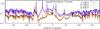Fig. 5

Ratio of scattered X-ray radiation (including HMXBs, LMXBs, and near-infrared-inferred low-luminosity sources) to the near-infrared-inferred GRXE profile for real sources for the energy ranges (from top to bottom) 3−10 keV, 10−20 keV, 17−25 keV, and 25−60 keV. The average spectrum of the LMXB sources in our calculations is significantly softer than the GRXE spectrum observed by RXTE and Integral (Revnivtsev et al. 2006; Krivonos et al. 2007a). As a result, the contribution of the scattered component to GRXE decreases at energies above 10 keV.

Fig. 6

Top panels: luminosity/sr radiated in our direction from the stellar GRXE and the scattered GRXE component (including stellar and XBs contributions) in the 3−20 keV range integrated over the longitude range (l< | 180°|) and latitude range − b to b. The difference in the scale height of the scattered component compared with a GRXE of stellar origin is clearly visible. Bottom panels: ratio of the two profiles. The peak in the ratio profile is caused by the elevation of the Sun above the Galactic plane by 15 pc.

The volume emissivity per unit solid angle due to scattering of this radiation at a distance s from the observer in the line of sight (l,b) is then given by $\begin{matrix} ϵ_{stellar} (s,ν) & = & \sum_{Z} $^{V} \frac{ρ_{GRXE} (x,y,z) f (ν)}{4 π d^{2} (x,y,z,s)} \end{matrix}$ $\begin{eqnarray} \nonumber \epsilon_{{\rm stellar}}(s, \nu) &= &\sum_{Z} \iiint\limits_V \frac{\rho_{{\rm GRXE}}(x,y,z)f(\nu)}{4\pi d^2(x,y,z,s)} \\ && \times \bigg(\frac{{\rm d}\sigma}{{\rm d}\Omega}(s, \nu) \bigg )_{Z} n_{Z}(s) {\rm d}V, \label{scatt_grxe_em} \end{eqnarray}$ (14)where ρ_GRXE is given in units of erg/cm³, d(x,y,z,s) is the distance from any point (x,y,z) in the Galaxy to the scattering point, and f(E) is the normalized spectral energy density taken from the GRXE spectrum given in Revnivtsev et al. (2006) and Krivonos et al. (2007a).

We show the contribution of this effect as an additional component to the longitude profiles given in Figs. 4 and 7. In the 3−20 keV energy range, the luminosity of GRXE is ≈1.4 × 10³⁸ ergs/s (Revnivtsev et al. 2006), which is lower than the luminosity of LMXBs (≈2.43 × 10³⁹ ergs/s), but higher than the luminosity of HMXBs (≈9 × 10³⁷ ergs/s), and this is clearly reflected in the contribution to the scattered X-ray intensity in Fig. 4. In the 17−60 keV energy range, the luminosity of the GRXE is 3.7 × 10³⁷ ergs/s (Krivonos et al. 2007a), which is a factor of ~5 lower than the luminosity of LMXBs (1.9 × 10³⁸ ergs/s) and a factor of ~2 lower than the luminosity of HMXBs (6.2 × 10³⁷ ergs/s). We therefore expect the scattering of the stellar component of the GRXE from the ISM to be subdominant, and this is evident in Fig. 4. The ratio of scattered X-rays to the GRXE inferred from near-infrared data is shown in Fig. 5. The diffuse scattered X-rays contribute 10 − 30% over most of the Galaxy with a contribution as high as 40% near the luminous sources in the 3−20 keV energy range. The diffuse component in the 17−60 keV range contributes, on the other hand, ~10% or less. This is low but still non-negligible.

Fig. 7

Longitude profiles of scattered XB radiation in comparison with near-infrared-inferred GRXE profile, in energy ranges 3−10 and 10−20 keV for Monte Carlo sources. If our Galaxy was on average more luminous in X-rays during the last several thousand years compared with the present, then the scattered component of the GRXE could be as bright as the stellar component. In reality, the scattered component strongly depends on the appearance of just a few new bright sources with luminosities close to the Eddington limit for a neutron star.

We calculate the luminosity/sr radiated in our direction from within a given latitude and longitude range in the sky dΩ (as opposed to the isotropic luminosity) for both the stellar GRXE and the scattered GRXE component as follows: $\begin{matrix} L_{GRXE, stellar} = \frac{1}{4 π} $ f (ν) ρ_{GRXE} (x,y,z) s^{2} d ν d s dΩ \\ L_{GRXE, scatt} = ” [ϵ_{XBs} (s,ν) + ϵ_{stellar} (s,ν)] s^{2} d ν d s dΩ, \end{matrix}$ $\begin{eqnarray} &&L_{{\rm GRXE,stellar}} = \frac{1}{4 \pi}\iiint f(\nu)\rho_{{\rm GRXE}}(x,y,z) s^2 {\rm d} \nu {\rm d} s {\rm d}\Omega \\ &&L_{{\rm GRXE,scatt}} = \iint [\epsilon_{{\rm XBs}}(s,\nu)+\epsilon_{{\rm stellar}}(s,\nu)] s^2 {\rm d} \nu {\rm d}s {\rm d}\Omega, \end{eqnarray}$ where the total volume emissivity due to scattering ϵ(s,ν) includes the contribution from both XB (Eq. (10)) and low-luminosity stellar source (Eq. (14))) components. The luminosity/sr profiles are plotted and compared in Fig. 6. The scattered radiation is on average ~10% as luminous as the stellar component of the GRXE in the inner ~1° of the Galactic plane.

5.3. Optimistic case: Monte Carlo simulated sources

Fig. 8

Ratio of scattered X-ray radiation (including HMXBs, LMXBs, and near-infrared-inferred low-luminosity sources) to the near-infrared-inferred GRXE profile for the Monte Carlo sources.

To consider the possibility that the current data significantly underestimate the average total luminosity of all the X-ray sources in the Galaxy, we use the Monte Carlo population of sources described below in the 3−20 keV range. The 2−10 keV luminosity of LMXBs, as discussed earlier, is 4.7 × 10³⁹ ergs/s, which is a factor of two higher than that of current data. The 2−10 keV luminosity of HMXBs is 1.7 × 10³⁹ ergs/s, which is almost a factor of 50 higher than what is currently observed. Compared with other galaxies, our Galaxy is therefore significantly underluminous (see e.g. Grimm et al. 2003; Lehmer et al. 2010; Mineo et al. 2012, 2014) even if we take a conservative star formation rate of 1 M_⊙/ yr. The results for scattered emission are shown in Fig. 7 in the form of longitude profiles at latitude b = 0°. As expected, in this case the scattered X-rays from the XBs account for almost all of the GRXE in the Galactic plane. This is clearer in the ratio of total scattered to observed GRXE shown in Fig. 8. Furthermore, recent estimates of the SFR in the Galaxy (Chomiuk & Povich 2011) seem to suggest a higher SFR (~1.9 M_⊙/ yr) than assumed in this work, which would imply an even higher discrepancy between the observed and expected luminosity of HMXBs. The contribution of scattered HMXBs could therefore be even higher than predicted by our simulated sample.

The observation of the diffuse component of the GRXE therefore provides a test of the hypothesis that our Galaxy is on average significantly more luminous than the current observations of the X-ray sources in the Galaxy suggest.

5.4. Comparison with the deep survey region of Revnivtsev et al. (2009)

The results of previous sections may seem to contradict the results of Revnivtsev et al. (2009), who resolved 80% of the GRXE into point sources. However, their field of view was located at latitude b = −1.42°. As discussed earlier, the scale height of the ISM is much lower (~0.6°), and therefore we expect the diffuse component of the GRXE to be significantly smaller at this latitude. We plot the latitude profile at l = 0.08° corresponding to the observation direction of Revnivtsev et al. (2009) and compare the GRXE profile inferred from near-infrared data (see Fig. 9). The scattered X-rays at b = −1.42 make up only 5% of the GRXE. Even in the optimistic case considered in the simulated population of sources, when the X-ray luminosity of the Galaxy is much higher, the diffuse contribution is ~26%. There is a coincidence here that a luminous Monte Carlo source lies nearby, giving a higher than average flux in this direction: the contribution on the other side of the Galactic plane at b = 1.42° is ~16%. This is consistent with the results of Revnivtsev et al. (2009). Therefore a significantly higher X-ray luminosity of Milky Way is allowed by current observations. The hypothesis that the average X-ray luminosity of our Galaxy is significantly higher than indicated by current data can be tested by studies similar to that of Revnivtsev et al. (2009), but conducted in the Galactic plane.

Recently, Morihana (2012) and Iso et al. (2012) have claimed that the resolved fraction in this field of view may be closer to 50%, allowing for a significantly larger contribution from the diffuse component. The analysis of Suzaku satellite data by Uchiyama et al. (2013) also allows for a contribution from the scattered radiation to the GRXE consistent with our predictions for the simulated optimistic case.

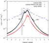Fig. 9

Latitude profiles of scattered XB radiation in comparison with the near-infrared-inferred GRXE profile in the energy range 3−10 keV for the field of view of 16 × 16 arcmin centered at l = 0.08°, b = −1.42°. In this region between 80 and 90% of the GRXE has been resolved into point sources (Revnivtsev et al. 2009). Percentages quoted show the fractional contribution of the diffuse GRXE component in each case. Because of the coincidental presence near this field of view of a luminous simulated source, we also quote the same value on the other side of the Galactic plane in the case of Monte Carlo sources.

Table 1

Comparison of XB scattered flux with ASCA measurements of 4−10 keV flux in the field of view of 20 GMC.

Fig. 10

Maps of diffuse X-ray emission from the ISM with HI modeled as a smooth disk and H2 using data from the Galactic Ring Survey in the energy ranges 3−10 keV (top panel), 10−20 keV (middle panel) and 17−60 keV (bottom panel). Giant molecular clouds are immediately evident.

5.5. Effect of the compactness of molecular clouds on the morphology of the diffuse GRXE

The GRS provides data for the spatial distribution, size and average density of 750 molecular clouds in the Galactic plane in the latitude range − 1° ≤ b ≤ 1° and the longitude range 18° ≤ ℓ ≤ 55.7°. This survey covers a part of one of the most significant concentrations of molecular gas in the Galaxy that is roughly distributed in a ring-like structure about 4 kpc from the Galactic center (Stecker et al. 1975; Cohen & Thaddeus 1977), although it may just be a spiral arm misinterpreted as a molecular ring (Dobbs & Burkert 2012). We assume that the density of each individual cloud is constant throughout the object. The total H2 mass of the clouds in the GRS is 3.5 × 10⁷M_⊙.

We account for the absorption of X-rays in the molecular cloud using photoabsorption cross-sections from Morrison & McCammon (1983). Scattering of X-rays from XBs on molecular clouds, which contain only a fraction of the total gas, gives a significant but patchy contribution to the GRXE. Part of the reason for this is that molecular clouds are dense and occupy a small volume (and angular area on the sky). Locally, along the lines of sight that intersect molecular clouds, they dominate the much smoother contribution from HI. In addition, there is a factor of 2 enhancement over atomic hydrogen (with same number density of H atoms) because of Rayleigh scattering for small scattering angles. We show the results after including the molecular clouds in the GRS instead of smooth distribution of molecular gas in Fig. 10. The molecular clouds are very obvious in these maps. This is even clearer in the latitude profiles shown in Fig. 11 along the direction tangent to the Scutum-Crux spiral arm of the Milky Way and the longitude profiles shown in Fig. 12. Even at relatively high latitudes, the molecular clouds are able to significantly contribute, locally, to the GRXE. This suggests that at high angular resolution, where we can resolve the molecular clouds, there should be significant fluctuations in the diffuse component of the GRXE, which would encode information about the distribution of molecular clouds in the Galaxy. The comparison of their contribution to the near-infrared-inferred GRXE is given in Fig. 13. The molecular clouds are evident as narrow peaks on small scales, in addition to broader peaks from the presence of luminous X-ray sources, and locally they are responsible for an increase of a factor of more than 2 in the diffuse component of GRXE compared with the average background.

We compare in Table 1 the results for the scattered flux from molecular clouds with the Advanced Satellite for Cosmology and Astrophysics (ASCA) (Tanaka et al. 1994) measurement of X-ray flux in the field of view of giant molecular clouds (GMC) (Cramphorn & Sunyaev 2002). The ASCA measurements provide an upper limit to the X-ray flux that might be produced by the scattering process. The scattered X-ray component is well below the limit set by ASCA. The X-ray telescopes Chandra and XMM-Newton (and Athena+ in the future) are significantly more sensitive than ASCA, which observed the giant molecular clouds in the Galactic plane for a relatively short time.

6. Contribution of LMXBs and HMXBs to the X-ray heating of the ISM

The competition between the different heating (e.g. from irradiation, cosmic rays, turbulent dissipation) and cooling processes (e.g. atomic lines such as CII,OI, Ly-α) plays a crucial role in determining the multiphase structure of the interstellar medium, formation of molecular clouds and star formation (Pikel’Ner 1968; Field et al. 1969; McKee & Ostriker 1977; Wolfire et al. 1995; Spitzer 1978; Cox 2005; Snow & McCall 2006; McKee & Ostriker 2007). The contribution of soft X-rays with energies ≲1 keV has been taken into account in standard calculations (Wolfire et al. 1995, 2003) assuming a quasi-homogeneous (smoothly varying with distance from the Galactic center) X-ray background. The heating from the soft X-rays, however, is confined to the outer layers of the clouds where they are almost completely absorbed. The harder X-rays at energies ≳1 keV can, on the other hand, penetrate the interiors of the HI and molecular clouds.X-ray binaries are the strongest sources of X-rays at these energies in galaxies similar to the Milky way, and should therefore have a significant effect on the structure and chemistry of the ISM. The contribution to the ISM heating from these sources should be highly variable both in space, for the obvious reason of the rapid decrease of the source’s X-ray flux with distance, and in time, because of the transient nature of most X-ray binaries.

The energy deposition rate from X-rays at a point in the Galaxy is given by $Γ_{x} = \sum_{i} \frac{L_{i} (ν)}{4 π R_{i}^{2}} [σ_{abs} (ν) - \sum_{Z} \frac{n_{Z}}{n_{H}} \frac{E_{K - α,Z}}{E_{ν}} Y_{Z} \times σ_{nl,Z} (ν)],$ $\begin{equation} \Gamma_x= \sum_{i} \frac{L_{i}(\nu)}{4\pi R^2_i} \bigg[\sigma_{{\rm abs}}(\nu) - \sum_{Z}\frac{n_Z}{n_{\rm H}}\frac{E_{{\rm K-}\alpha,Z}}{E_{\nu}}Y_{Z}\times \sigma_{nl,Z}(\nu) \bigg], \label{emissivity} \end{equation}$ (17)where the sum computed is over the X-ray sources i, R_i is the distance of the source to the point of absorption and L_i is its luminosity, σ_abs is the photoelectric absorption cross-section given in Morrison & McCammon (1983), the sum Z over heavy elements includes O, Fe, C, Ne, Si, Mg, σ_abs,Z is the analytic fit to the partial photoionisation cross-section of the n = 1,l = 0 state of element Z as given in Verner & Yakovlev (1995), Y_Z is the K-α yield, E_{K − α,Z} is the energy of the K-α line, and n_Z/n_H is the relative abundance for solar abundance estimates considered in Morrison & McCammon (1983). Above 10 keV we use the partial K-shell ionization cross-sections of Fe and Ni, which dominate the absorption cross-section at these energies.

Fig. 11

Latitude profile of scattered XB radiation near the line of sight tangential to one of the spiral arms (Scutum-Crux). The lines of sight passing through giant molecular clouds can receive a significantly higher contribution (than the average background) from the scattered X-rays.

Fig. 12

Comparison of longitude profiles of scattered XB radiation in different energy ranges including effects of molecular clouds (visible as narrow peaks in the profiles) for the energy ranges (from top to bottom) 3−10 keV, 10−20 keV, 17-25keV and 25−60 keV.

Fig. 13

Ratio of longitude profiles of scattered XB radiation in different energy ranges including effects of molecular clouds (visible as narrow peaks in the profiles) to the near-infrared-inferred GRXE emission for the energy ranges (from top to bottom) 3−10 keV, 10−20 keV, 17−25keV and 25−60 keV.

We plot the energy deposited by photoabsorption of X-rays in Fig. 14 as profiles along the x-axes for different cuts along the y-axes in the Galactic plane, with coordinates for the Galactic center at (x,y) = (0,0) and position of the Sun at (x,y) = ( − 8,0) kpc. Not all the energy absorbed from the X-rays will go into heating the clouds, as some of it will be radiated away as low-energy photons coming from excitations and ionization and subsequent recombinations of atoms (Shull & van Steenberg 1985). The conversion of the X-ray energy into heat will in particular be most efficient if the ionization fraction is large so that most of the initially absorbed energy is dissipated via distant electron-electron collisions and not through excitations. In addition, most of the initially absorbed X-ray energy (minus the energy that escapes via the fluorescent K-α,β lines of Fe and Ni) will be converted in heat if the hydrogen column density or the dust opacity is so high that photons with energy Ly-α or higher (≳10.2 eV) cannot escape. For the discussion below we assume, for the sake of comparison, that one or more of these conditions holds and that most of the X-ray energy is absorbed. In reality, the fraction will vary significantly depending upon the local conditions (Shull & van Steenberg 1985).

For reference we plot the heating rate from CXB using the spectral fit of Gruber et al. (1999) and integrating up to 60 keV, although the contribution from energies ≳10 keV is negligible. In addition to the photoabsorption, hard X-rays also transfer energy to the gas when they Compton-scatter on electrons, both free and bound in hydrogen and helium, through the recoil effect. The average energy transferred by a photon of energy E is E × E/ (m_ec²), where m_e is the mass of the electron and c is the speed of light in vacuum (see e.g. Pozdnyakov et al. 1983). The average energy deposition rate is therefore given by Γ_recoil = ∫dEF_Xσ_KNE/ (m_ec²) (1−2.2E/ (m_ec²)), where F_X is the specific X-ray flux in units of (ergs/s/cm²/ keV) and σ_KN is the Klein-Nishina cross-section; we include the lowest-order Klein-Nishina correction to the average recoil energy. For solar metallicity, taking log Fe = 7.52 normalized to log H = 12 used in Morrison & McCammon (1983), the heating from recoil dominates the heating from photoabsorption at ≈28 keV. For CXB the contribution of the recoil effect to the heating rate is ≈4 × 10^-32 ergs/s/electron, counting free electrons as well as those bound in hydrogen and helium and in the outer shells of heavier elements. In general, therefore, we expect the recoil effect to be negligible, but it might become important in the vicinity of the hard X-ray sources. The CXB, in contrast to X-ray binaries, uniformly heats the intergalactic medium everywhere. The energy density in CXB peaks around z ~ 0.7−1 (Ueda et al. 2003; Hasinger et al. 2005; Barger et al. 2005) and its contribution is therefore more important in high redshift galaxies.

Fig. 14

Heating of the ISM per hydrogen atom from photoabsorption of X-rays from LMXBs (left panel) and HMXBs (right panel). For comparison the contribution from cosmic rays following Spitzer (1978) and Wolfire et al. (2003) and CXB is also shown. The X-ray (≳1 keV) contribution dominates compared with the cosmic rays (assuming the same energy density as the solar neighborhood) in a significant part of the Galaxy.

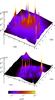Fig. 15

Three-dimensional maps of the heating of the ISM per hydrogen atom from photoabsorption of X-rays from LMXBs, HMXBs and CXB on the Galactic plane for Monte Carlo sources (top panel) and real sources (bottom panel). In the outer regions of the Galaxy the heating rate approaches the lower bound of ~1.9 × 10^-29 ergs/s/HI coming from absorbed CXB photons. The green cross indicates the position of the Galactic center in each map.

An important point to note is that the area of influence of luminous sources extends quite far, up to a few kpc away from the source for the most luminous sources. These heating rates need to be compared with the heating rate from the cosmic rays estimated to be, on average in the solar neighborhood, Γ_CR ≈ 10^-28 erg/s/HI and also with typical heating rates from photoelectric heating by dust grains. The X-ray heating is comparable with and even stronger than the cosmic ray heating (assuming a solar neighbourhood energy density) in a significant part of the Galaxy and may be higher than other heating mechanisms typically considered. The optimistic case, where the X-ray luminosity of the Milky Way is scaled to match the activity in the other galaxies, is shown in Fig. 15 using the Monte Carlo sources. The X-ray heating dominates over the solar neighbourhood energy density of cosmic rays in almost the whole Galaxy and if Milky Way activity in the past was close to this level, X-ray heating would have played an important role in the energetics of the different phases of the ISM. The star-forming galaxies have a much higher X-ray luminosity than even this optimistic case for the Milky Way and the X-ray heating therefore very likely plays a crucial role in the evolution of their ISM.

7. Conclusions

Weak X-ray sources such as cataclysmic variables (CVs) and coronally active binaries are currently believed to be the main contributors to the GRXE. We investigate the scattering by the interstellar medium of X-rays produced by Galactic X-ray sources as a possible truly diffuse component of the GRXE emission. We include contributions from coherent scattering from molecular hydrogen, helium and heavy elements in addition to the atomic hydrogen. The scattering of X-rays from luminous sources results in bright regions around the sources, the proximity zones, similar to the dust halos, but extending to much larger scattering angles than the ≲1° for dust halos. The scattered photons from the ISM originating in the known X-ray binary sources and stellar sources in the Galaxy are able to contribute, on average, 10 − 30% of the flux currently identified as GRXE in the Galactic plane. The profile of the scattered intensity follows the distribution of gas in the Galaxy with a scale height of 80 pc (0.6° at 8 kpc distance), which is much sharper than the profile of stellar distribution with a scale height of ~130 pc. Therefore we expect the stellar point sources to dominate away from the Galactic plane, while the scattered X-rays would be concentrated within the central 1° of the plane. Molecular clouds locally enhance the scattered intensity, imprinting their morphology on the GRXE. The coherent scattering by electrons in the molecular hydrogen operates on a comparatively wide range of scattering angles at low energies than at high energies, making the scattered spectrum softer than the incident spectrum (see Appendix C).

We also find that the X-rays from the luminous binary sources contribute significantly to the heating rate in the interstellar medium, especially in the interiors of the clouds where the UV or softer X-rays are unable to penetrate. This important effect has so far been ignored in the standard studies of the multiphase ISM (McKee & Ostriker 1977; Wolfire et al. 1995, 2003). This effect would be even stronger at high redshifts (z ~ 0.7 − 1) where the CXB energy density peaks and is much higher than today as well as in star-forming galaxies, which have a much higher X-ray luminosity than the Milky Way.

We only calculate the X-ray flux integrated over particular X-ray bands because this will be more readily observable in reasonable observation time with telescopes in operation now or expected in the near future, such as NuSTAR (Harrison et al. 2013), Spectrum-RG/ART-XC (Pavlinsky et al. 2008) and Astro-H (Takahashi et al. 2010). There is additional information in the spectrum of the scattered emission that may help to distinguish between the scattered GRXE and stellar GRXE. Of particular interest in this regard is the emission of fluorescent lines of neutral elements such as iron, sulphur and silicon. We have also assumed that the sources are persistent. The transient nature of most X-ray binary sources as well as extreme events such as gamma-ray bursts and giant flares from magnetars will leave unique signatures in the morphology of the scattered GRXE. We will consider these effects in a separate publication (Khatri & Sunyaev, in prep.).

Compared with other galaxies, the Milky Way is underluminous in X-rays according to current observations. It is possible that the Milky Way is just going through a phase of low X-ray activity at present but was more luminous in the past. In particular, if the time-averaged luminosity of Milky Way is the same as inferred from averaged relations between X-ray luminosity and star formation rate/stellar mass of other galaxies, then the scattered component will on average contribute to more than 50% to the GRXE in the galactic plane and would dominate the stellar component in a significant part of the Galaxy. This hypothesis is allowed by current observations and is testable by observations of the Galactic plane with high angular resolution and sensitivity, similar to the study by Revnivtsev et al. (2009) below the Galactic plane.

Online material

Appendix A: List of LMXB and HMXB sources used in the calculations

Full list of sources used in the calculations with the corresponding data (also available at http://www.mpa-garching.mpg.de/~molaro).

Table A.1

List of sources used in the calculations, ranked by 2−10 keV luminosity.

Appendix B: Contribution of Sgr A^∗

As discussed in Sect. 2, the past activity of the currently low quiescent source Sgr A^∗ might have significantly contributed to the cumulative X-ray output of the Galaxy, and hence to the diffuse GRXE component. In Fig. B.1 we show the minimum luminosity required for the flux from this source to outshine the contribution of the entire XBs population at different positions on the Galactic plane, estimated as $L_{Sgr A^{*}} = 4 π R_{Sgr A^{*}}^{2} \times \sum_{i} \frac{L_{i} (ν)}{4 π R_{i}^{2}} \cdot$ $\appendix \setcounter{section}{2} \begin{equation} L_{{\rm Sgr} A^*} = 4 \pi R^2_{{\rm Sgr} A^*} \times \sum_{i} \frac{L_{i}(\nu)}{4\pi R^2_i}\cdot \end{equation}$ (B.1)

Fig. B.1

Minimum Sgr A^∗ luminosity required for the source’s flux to be higher than the total HMXBs (left panel) and LMXBs (right panel) contribution at different positions on the Galactic plane. If we know the star formation rate and the mass of a galaxy, we can estimate the X-ray luminosity contributed by the X-ray binaries and similarly find when the AGNs contribute more than the X-ray binaries to the heating of the gas in other galaxies with AGNs.

Appendix C: Scattering cross-sections

In Fig. C.1 we illustrate the energy dependence of the scattering cross-section for the case of H2 scattering. In Figs. C.2 and C.3 we highlight the additional effects caused by bound electrons by showing the ratio of contributions from H2 and He with respect to the free electrons. The energy dependence of Rayleigh scattering is clearly evident. At high energies, Rayleigh scattering operates only on a very narrow range of scattering angles and the total scattering cross-section approaches the Klein-Nishina cross-section. At low energies, coherent Rayleigh scattering results in the enhancement of the cross section for a significant range of scattering angles, resulting in a higher average scattering rate of low-energy photons. The average scattered spectrum is therefore softer than the average incident spectrum. The contribution of molecular hydrogen as well as helium and heavier elements is compared in Table C.1 in the Rayleigh scattering limit (0° scattering angle). The elements heavier than helium contribute ≲10% in this extreme case, and the actual contribution when suitably averaged over different scattering angles would be smaller than the values in the table.

Fig. C.1

Cross-section (Rayleigh+ Compton) in polar coordinates, σ(θ)e^iθ, where σ is the amplitude of the cross-section in units of $r_{e}^{2}$ $\hbox{$r_{\rm e}^2$}$ for the scattering angle θ and r_e is the classical electron radius. The enhancement of Rayleigh scattering caused by coherence effects is clearly visible at low energies. While the cross section remains constant with energy at angles close to zero, the contribution of Rayleigh scattering is shown to quickly decrease with increasing energy. Compton scattering is also suppressed by relativistic effects.

Near the Galactic center, a luminosity of ≳10³⁷ erg/s from Sgr A^∗ would be enough to become comparable with the illumination from X-ray binaries. On the outskirts of the Galaxy, on the other hand, Sgr A^∗, or some other ultra-luminous source near the Galactic center, can be ignored as long as its luminosity is ≲10³⁹−10⁴⁰ erg/s.

Fig. C.2

Ratio of the Rayleigh + Compton differential cross-section of H2 + He to HI + He (where each element is weighted by relative abundance) as a function of energy for different scattering angles. The total cross section approaches that of unbound electrons as the importance of coherence effects decreases with energy, because of the suppression of Rayleigh scattering.

Table C.1

Elements according to maximal contribution to Rayleigh scattering if all hydrogen is in atomic form (or molecular form, given in parentheses).

Fig. C.3

Ratio of intensity from the Monte Carlo simulated HMXBs (left column) and LMXBs (right column) scattered along the Galactic plane (b = 0) by H2 (top row) and He (bottom row) to the intensity that would be scattered if all electrons were unbound. The range of scattering angles over which the Rayleigh scattering dominates the scattering cross section depends on the characteristic size of the electron distribution in the atom or molecule, which differs for different elements and molecules (see Sect. 4.1). This leads to a nonlinear dependence of the ratio of cross sections for different elements and molecules on the scattering angle. At each longitude many different scattering angles contribute, corresponding to the relative position of the X-ray sources w.r.t. the gas along the line of sight, resulting in the apparent longitudinal dependence of the ratio profiles.

¹

The full catalog of sources used can be found in Appendix A and at http://www.mpa-garching.mpg.de/~molaro

²

See http://edoc.ub.uni-muenchen.de/1279/1/Grimm_Hans-Jakob.pdf for the full list of sources and associated data.

³

We do not include the contribution of the Crab nebula, which because it is only ~1000 years old would only contribute a small peak near the Galactic anti-center.

⁴

Available on the LAMBDA archive at http://lambda.gsfc.nasa.gov

Acknowledgments

We would like to thank Mike Revnivtsev for discussions and Ken Ebisawa, Marat Gilfanov, Christopher Mckee, Jeremiah Ostriker, and Scott Tremaine for comments on the manuscript. This research has made use of the SIMBAD database, operated at CDS, Strasbourg, France.

References

Asplund, M., Grevesse, N., Sauval, A. J., & Scott, P. 2009, ARA&A, 47, 481 [NASA ADS] [CrossRef] [Google Scholar]
Baganoff, F. K., Maeda, Y., Morris, M., et al. 2003, ApJ, 591, 891 [NASA ADS] [CrossRef] [Google Scholar]
Bahcall, J. N., & Soneira, R. M. 1980, ApJS, 44, 73 [NASA ADS] [CrossRef] [Google Scholar]
Bandyopadhyay, R. M., Shahbaz, T., Charles, P. A., & Naylor, T. 1999, MNRAS, 306, 417 [NASA ADS] [CrossRef] [Google Scholar]
Barger, A. J., Cowie, L. L., Mushotzky, R. F., et al. 2005, AJ, 129, 578 [NASA ADS] [CrossRef] [Google Scholar]
Bassa, C. G., Jonker, P. G., in’tZand, J. J. M., & Verbunt, F. 2006, A&A, 446, L17 [NASA ADS] [CrossRef] [EDP Sciences] [Google Scholar]
Baykal, A., Stark, M. J., & Swank, J. H. 2002, ApJ, 569, 903 [NASA ADS] [CrossRef] [Google Scholar]
Bergstrom, P. M., Surić, T., Pisk, K., & Pratt, R. H. 1993, Phys. Rev. A, 48, 1134 [NASA ADS] [CrossRef] [PubMed] [Google Scholar]
Bhattacharyya, S., Strohmayer, T. E., Markwardt, C. B., & Swank, J. H. 2006, ApJ, 639, L31 [NASA ADS] [CrossRef] [Google Scholar]
Binney, J., & Tremaine, S. 2008, Galactic Dynamics: 2nd edn. (Princeton University Press) [Google Scholar]
Blitz, L. 1993, in Protostars and Planets III, eds. E. H. Levy, & J. I. Lunine, 125 [Google Scholar]
Capelli, R., Warwick, R. S., Porquet, D., Gillessen, S., & Predehl, P. 2012, A&A, 545, A35 [NASA ADS] [CrossRef] [EDP Sciences] [Google Scholar]
Cartwright, T. F., Engel, M. C., Heinke, C. O., et al. 2013, ApJ, 768, 183 [NASA ADS] [CrossRef] [Google Scholar]
Chaty, S., Mignani, R. P., & Israel, G. L. 2006, MNRAS, 365, 1387 [NASA ADS] [CrossRef] [Google Scholar]
Chen, Y.-P., Zhang, S., Torres, D. F., Wang, J.-M., & Li, T.-P. 2010, A&A, 510, A81 [NASA ADS] [CrossRef] [EDP Sciences] [Google Scholar]
Chenevez, J., Falanga, M., Kuulkers, E., et al. 2007, A&A, 469, L27 [NASA ADS] [CrossRef] [EDP Sciences] [Google Scholar]
Chomiuk, L., & Povich, M. S. 2011, AJ, 142, 197 [NASA ADS] [CrossRef] [Google Scholar]
Christian, D. J., & Swank, J. H. 1997, ApJS, 109, 177 [NASA ADS] [CrossRef] [Google Scholar]
Clavel, M., Terrier, R., Goldwurm, A., et al. 2013, A&A, 558, A32 [NASA ADS] [CrossRef] [EDP Sciences] [Google Scholar]
Cohen, R. S., & Thaddeus, P. 1977, ApJ, 217, L155 [NASA ADS] [CrossRef] [Google Scholar]
Colbert, E. J. M., Heckman, T. M., Ptak, A. F., Strickland, D. K., & Weaver, K. A. 2004, ApJ, 602, 231 [NASA ADS] [CrossRef] [Google Scholar]
Coleiro, A., & Chaty, S. 2013, ApJ, 764, 185 [NASA ADS] [CrossRef] [Google Scholar]
Corbel, S., Kaaret, P., Fender, R. P., et al. 2005, ApJ, 632, 504 [NASA ADS] [CrossRef] [Google Scholar]
Cox, D. P. 2005, ARA&A, 43, 337 [NASA ADS] [CrossRef] [EDP Sciences] [MathSciNet] [Google Scholar]
Cramphorn, C. K., & Sunyaev, R. A. 2002, A&A, 389, 252 [NASA ADS] [CrossRef] [EDP Sciences] [Google Scholar]
Dame, T. M., Hartmann, D., & Thaddeus, P. 2001, ApJ, 547, 792 [NASA ADS] [CrossRef] [Google Scholar]
Degenaar, N., Jonker, P. G., Torres, M. A. P., et al. 2010, MNRAS, 404, 1591 [NASA ADS] [Google Scholar]
Dehnen, W., & Binney, J. 1998, MNRAS, 294, 429 [NASA ADS] [CrossRef] [Google Scholar]
Del Santo, M., Chenevez, J., Brandt, S., Bazzano, A., & Ubertini, P. 2007, ATel, 1207, 1 [Google Scholar]
Dobbs, C. L., & Burkert, A. 2012, MNRAS, 421, 2940 [NASA ADS] [CrossRef] [Google Scholar]
Doroshenko, R. F., Doroshenko, V. A., Postnov, K. A., Cherepashchuk, A. M., & Tsygankov, S. S. 2007, in ESA SP, 622, 495 [Google Scholar]
Doroshenko, V., Suchy, S., Santangelo, A., et al. 2010, A&A, 515, L1 [NASA ADS] [CrossRef] [EDP Sciences] [Google Scholar]
Dotani, T., Asai, K., & Wijnands, R. 2000, ApJ, 543, L145 [NASA ADS] [CrossRef] [Google Scholar]
Draine, B. T. 2011, Physics of the Interstellar and Intergalactic Medium (Princeton University Press) [Google Scholar]
Dwek, E., Arendt, R. G., Hauser, M. G., et al. 1995, ApJ, 445, 716 [CrossRef] [Google Scholar]
Ebisawa, K., Maeda, Y., Kaneda, H., & Yamauchi, S. 2001, Science, 293, 1633 [NASA ADS] [CrossRef] [PubMed] [Google Scholar]
Ebisawa, K., Tsujimoto, M., Paizis, A., et al. 2005, ApJ, 635, 214 [NASA ADS] [CrossRef] [Google Scholar]
Ebisawa, K., Yamauchi, S., Tanaka, Y., et al. 2008, PASJ, 60, 223 [NASA ADS] [Google Scholar]
Eisenberger, P., & Platzman, P. M. 1970, Phys. Rev. A, 2, 415 [NASA ADS] [CrossRef] [Google Scholar]
Falanga, M., Bonnet-Bidaud, J. M., Poutanen, J., et al. 2005a, A&A, 436, 647 [NASA ADS] [CrossRef] [EDP Sciences] [Google Scholar]
Falanga, M., Kuiper, L., Poutanen, J., et al. 2005b, A&A, 444, 15 [NASA ADS] [CrossRef] [EDP Sciences] [Google Scholar]
Field, G. B., Goldsmith, D. W., & Habing, H. J. 1969, ApJ, 155, L149 [NASA ADS] [CrossRef] [Google Scholar]
Filippova, E. V., Tsygankov, S. S., Lutovinov, A. A., & Sunyaev, R. A. 2005, Astron. Lett., 31, 729 [NASA ADS] [CrossRef] [Google Scholar]
Freudenreich, H. T. 1996, ApJ, 468, 663 [NASA ADS] [CrossRef] [Google Scholar]
Galloway, D. K., Psaltis, D., Muno, M. P., & Chakrabarty, D. 2006, ApJ, 639, 1033 [NASA ADS] [CrossRef] [Google Scholar]
Gando Ryu, S., Nobukawa, M., Nakashima, S., et al. 2012, PASJ, accepted [arXiv:1211.4529] [Google Scholar]
Giacconi, R., Gursky, H., Paolini, F. R., & Rossi, B. B. 1962, Phys. Rev. Lett., 9, 439 [NASA ADS] [CrossRef] [Google Scholar]
Gilfanov, M. 2004, MNRAS, 349, 146 [NASA ADS] [CrossRef] [Google Scholar]
Gilfanov, M., Revnivtsev, M., & Molkov, S. 2003, A&A, 410, 217 [NASA ADS] [CrossRef] [EDP Sciences] [Google Scholar]
Gilfanov, M., Grimm, H.-J., & Sunyaev, R. 2004, MNRAS, 351, 1365 [NASA ADS] [CrossRef] [Google Scholar]
Grimm, H.-J. 2003, Ph.D. Thesis, Ludwig Maximilian University of Munich [Google Scholar]
Grimm, H.-J., Gilfanov, M., & Sunyaev, R. 2002, A&A, 391, 923 [NASA ADS] [CrossRef] [EDP Sciences] [Google Scholar]
Grimm, H.-J., Gilfanov, M., & Sunyaev, R. 2003, MNRAS, 339, 793 [NASA ADS] [CrossRef] [Google Scholar]
Gruber, D. E., Matteson, J. L., Peterson, L. E., & Jung, G. V. 1999, ApJ, 520, 124 [NASA ADS] [CrossRef] [Google Scholar]
Haardt, F., Galli, M. R., Treves, A., et al. 2001, ApJS, 133, 187 [NASA ADS] [CrossRef] [Google Scholar]
Harrison, F. A., Craig, W. W., Christensen, F. E., et al. 2013, ApJ, 770, 103 [NASA ADS] [CrossRef] [Google Scholar]
Hasinger, G., Miyaji, T., & Schmidt, M. 2005, A&A, 441, 417 [NASA ADS] [CrossRef] [EDP Sciences] [Google Scholar]
Hubbell, J. H., Veigele, W. J., Briggs, E. A., et al. 1975, J. Phys. Chem. Ref. Data, 4, 471 [NASA ADS] [CrossRef] [Google Scholar]
Hynes, R. I., Steeghs, D., Casares, J., Charles, P. A., & O’Brien, K. 2004, ApJ, 609, 317 [NASA ADS] [CrossRef] [Google Scholar]
Iaria, R., di Salvo, T., Robba, N. R., et al. 2005, A&A, 439, 575 [NASA ADS] [CrossRef] [EDP Sciences] [Google Scholar]
in’t Zand, J. J. M., Verbunt, F., Kuulkers, E., et al. 2002, A&A, 389, L43 [NASA ADS] [CrossRef] [EDP Sciences] [Google Scholar]
in’t Zand, J. J. M., Kuulkers, E., Verbunt, F., Heise, J., & Cornelisse, R. 2003, A&A, 411, L487 [NASA ADS] [CrossRef] [EDP Sciences] [Google Scholar]
in’t Zand, J. J. M., Cornelisse, R., & Méndez, M. 2005, A&A, 440, 287 [NASA ADS] [CrossRef] [EDP Sciences] [Google Scholar]
Inui, T., Koyama, K., Matsumoto, H., & Tsuru, T. G. 2009, PASJ, 61, 241 [Google Scholar]
Iso, N., Ebisawa, K., & Tsujimoto, M. 2012, in AIP Conf. Ser. 1427, eds. R. Petre, K. Mitsuda, & L. Angelini, 288 [Google Scholar]
Israel, G. L., Negueruela, I., Campana, S., et al. 2001, A&A, 371, 1018 [NASA ADS] [CrossRef] [EDP Sciences] [Google Scholar]
Jackson, J. M., Rathborne, J. M., Shah, R. Y., et al. 2006, ApJS, 163, 145 [NASA ADS] [CrossRef] [Google Scholar]
Jonker, P. G., & Nelemans, G. 2004, MNRAS, 354, 355 [NASA ADS] [CrossRef] [Google Scholar]
Kalberla, P. M. W., & Kerp, J. 2009, ARA&A, 47, 27 [NASA ADS] [CrossRef] [Google Scholar]
Kalberla, P. M. W., Burton, W. B., Hartmann, D., et al. 2005, A&A, 440, 775 [NASA ADS] [CrossRef] [EDP Sciences] [Google Scholar]
Kennea, J. A., & Campana, S. 2006, ATel, 818, 1 [NASA ADS] [Google Scholar]
Kent, S. M., Dame, T. M., & Fazio, G. 1991, ApJ, 378, 131 [NASA ADS] [CrossRef] [Google Scholar]
Kinugasa, K., Torii, K., Hashimoto, Y., et al. 1998, ApJ, 495, 435 [NASA ADS] [CrossRef] [Google Scholar]
Kong, A. K. H., Homer, L., Kuulkers, E., Charles, P. A., & Smale, A. P. 2000, MNRAS, 311, 405 [NASA ADS] [CrossRef] [Google Scholar]
Koyama, K., Makishima, K., Tanaka, Y., & Tsunemi, H. 1986, PASJ, 38, 121 [NASA ADS] [Google Scholar]
Koyama, K., Awaki, H., Kunieda, H., Takano, S., & Tawara, Y. 1989, Nature, 339, 603 [NASA ADS] [CrossRef] [Google Scholar]
Koyama, K., Maeda, Y., Sonobe, T., et al. 1996, PASJ, 48, 249 [NASA ADS] [CrossRef] [Google Scholar]
Koyama, K., Hyodo, Y., Inui, T., et al. 2007, PASJ, 59, 245 [NASA ADS] [Google Scholar]
Krivonos, R., Revnivtsev, M., Churazov, E., et al. 2007a, A&A, 463, 957 [NASA ADS] [CrossRef] [EDP Sciences] [Google Scholar]
Krivonos, R., Revnivtsev, M., Lutovinov, A., et al. 2007b, A&A, 475, 775 [NASA ADS] [CrossRef] [EDP Sciences] [Google Scholar]
Krivonos, R., Tsygankov, S., Lutovinov, A., et al. 2012, A&A, 545, A27 [NASA ADS] [CrossRef] [EDP Sciences] [Google Scholar]
Kuulkers, E., den Hartog, P. R., in’t Zand, J. J. M., et al. 2003, A&A, 399, 663 [NASA ADS] [CrossRef] [EDP Sciences] [Google Scholar]
Lehmer, B. D., Alexander, D. M., Bauer, F. E., et al. 2010, ApJ, 724, 559 [NASA ADS] [CrossRef] [Google Scholar]
Levine, E. S., Blitz, L., & Heiles, C. 2006, Science, 312, 1773 [NASA ADS] [CrossRef] [Google Scholar]
Lin, D., Homan, J., Remillard, R., & Wijnands, R. 2007, ATel, 1183, 1 [NASA ADS] [Google Scholar]
Liu, Q. Z., van Paradijs, J., & van den Heuvel, E. P. J. 2006, A&A, 455, 1165 [NASA ADS] [CrossRef] [EDP Sciences] [Google Scholar]
Liu, Q. Z., van Paradijs, J., & van den Heuvel, E. P. J. 2007, A&A, 469, 807 [NASA ADS] [CrossRef] [EDP Sciences] [Google Scholar]
Lowell, A. W., Tomsick, J. A., Heinke, C. O., et al. 2012, ApJ, 749, 111 [NASA ADS] [CrossRef] [Google Scholar]
Lutovinov, A., Revnivtsev, M., Gilfanov, M., et al. 2005a, A&A, 444, 821 [NASA ADS] [CrossRef] [EDP Sciences] [Google Scholar]
Lutovinov, A., Revnivtsev, M., Molkov, S., & Sunyaev, R. 2005b, A&A, 430, 997 [NASA ADS] [CrossRef] [EDP Sciences] [Google Scholar]
Lutovinov, A. A., Revnivtsev, M. G., Tsygankov, S. S., & Krivonos, R. A. 2013, MNRAS, 431, 327 [NASA ADS] [CrossRef] [Google Scholar]
Lyubimkov, L. S., Rostopchin, S. I., Roche, P., & Tarasov, A. E. 1997, MNRAS, 286, 549 [NASA ADS] [CrossRef] [Google Scholar]
Macomb, D. J., & Gehrels, N. 1999, ApJS, 120, 335 [NASA ADS] [CrossRef] [Google Scholar]
Mangano, V., Romano, P., Sidoli, L., et al. 2008, ATel, 1727, 1 [NASA ADS] [Google Scholar]
Markwardt, C. B., Strohmayer, T. E., & Swank, J. H. 2008, ATel, 1443, 1 [NASA ADS] [Google Scholar]
Masetti, N., Morelli, L., Palazzi, E., et al. 2006a, A&A, 459, 21 [Google Scholar]
Masetti, N., Pretorius, M. L., Palazzi, E., et al. 2006b, A&A, 449, 1139 [NASA ADS] [CrossRef] [EDP Sciences] [Google Scholar]
Mason, K. O., & Cordova, F. A. 1982, ApJ, 262, 253 [NASA ADS] [CrossRef] [Google Scholar]
Mauche, C. W., & Gorenstein, P. 1986, ApJ, 302, 371 [NASA ADS] [CrossRef] [Google Scholar]
McClure-Griffiths, N. M., Pisano, D. J., Calabretta, M. R., et al. 2009, ApJS, 181, 398 [NASA ADS] [CrossRef] [Google Scholar]
McKee, C. F., & Ostriker, E. C. 2007, ARA&A, 45, 565 [NASA ADS] [CrossRef] [Google Scholar]
McKee, C. F., & Ostriker, J. P. 1977, ApJ, 218, 148 [NASA ADS] [CrossRef] [Google Scholar]
McMillan, P. J. 2011, MNRAS, 414, 2446 [NASA ADS] [CrossRef] [Google Scholar]
Mereghetti, S., Tiengo, A., Israel, G. L., & Stella, L. 2000, A&A, 354, 567 [NASA ADS] [Google Scholar]
Migliari, S., Di Salvo, T., Belloni, T., et al. 2003, MNRAS, 342, 909 [NASA ADS] [CrossRef] [Google Scholar]
Mineo, S., Gilfanov, M., & Sunyaev, R. 2012, MNRAS, 419, 2095 [NASA ADS] [CrossRef] [Google Scholar]
Mineo, S., Gilfanov, M., Lehmer, B. D., Morrison, G. E., & Sunyaev, R. 2014, MNRAS, 437, 1698 [NASA ADS] [CrossRef] [Google Scholar]
Misiriotis, A., Xilouris, E. M., Papamastorakis, J., Boumis, P., & Goudis, C. D. 2006, A&A, 459, 113 [NASA ADS] [CrossRef] [EDP Sciences] [Google Scholar]
Morihana, K. 2012, PASP, 124, 1132 [NASA ADS] [CrossRef] [Google Scholar]
Morihana, K., Tsujimoto, M., Yoshida, T., & Ebisawa, K. 2013, ApJ, 766, 14 [NASA ADS] [CrossRef] [Google Scholar]
Morrison, R., & McCammon, D. 1983, ApJ, 270, 119 [NASA ADS] [CrossRef] [Google Scholar]
Muno, M. P., Baganoff, F. K., Bautz, M. W., et al. 2004, ApJ, 613, 326 [NASA ADS] [CrossRef] [Google Scholar]
Muno, M. P., Baganoff, F. K., Brandt, W. N., Park, S., & Morris, M. R. 2007, ApJ, 656, L69 [NASA ADS] [CrossRef] [Google Scholar]
Murakami, H., Koyama, K., Sakano, M., Tsujimoto, M., & Maeda, Y. 2000, ApJ, 534, 283 [NASA ADS] [CrossRef] [Google Scholar]
Nagata, T., Kato, D., Baba, D., et al. 2003, PASJ, 55, L73 [NASA ADS] [Google Scholar]
Naik, S., & Paul, B. 2004, A&A, 418, 655 [NASA ADS] [CrossRef] [EDP Sciences] [Google Scholar]
Narayan, R., Mahadevan, R., Grindlay, J. E., Popham, R. G., & Gammie, C. 1998, ApJ, 492, 554 [NASA ADS] [CrossRef] [Google Scholar]
Natalucci, L., Bazzano, A., Cocchi, M., et al. 2000, ApJ, 536, 891 [NASA ADS] [CrossRef] [Google Scholar]
Negueruela, I., & Okazaki, A. T. 2001, A&A, 369, 108 [NASA ADS] [CrossRef] [EDP Sciences] [Google Scholar]
Negueruela, I., Roche, P., Fabregat, J., & Coe, M. J. 1999, MNRAS, 307, 695 [NASA ADS] [CrossRef] [Google Scholar]
Negueruela, I., Smith, D. M., Harrison, T. E., & Torrejón, J. M. 2006, ApJ, 638, 982 [NASA ADS] [CrossRef] [Google Scholar]
Nobukawa, M., Ryu, S. G., Tsuru, T. G., & Koyama, K. 2011, ApJ, 739, L52 [NASA ADS] [CrossRef] [Google Scholar]
Oosterbroek, T., Barret, D., Guainazzi, M., & Ford, E. C. 2001, A&A, 366, 138 [NASA ADS] [CrossRef] [EDP Sciences] [Google Scholar]
Overbeck, J. W. 1965, ApJ, 141, 864 [NASA ADS] [CrossRef] [Google Scholar]
Paerels, F., Brinkman, A. C., van der Meer, R. L. J., et al. 2001, ApJ, 546, 338 [NASA ADS] [CrossRef] [Google Scholar]
Papitto, A., Menna, M. T., Burderi, L., di Salvo, T., & Riggio, A. 2008, MNRAS, 383, 411 [NASA ADS] [CrossRef] [Google Scholar]
Parmar, A. N., Gottwald, M., van der Klis, M., & van Paradijs, J. 1989, ApJ, 338, 1024 [NASA ADS] [CrossRef] [Google Scholar]
Parmar, A. N., Oosterbroek, T., Sidoli, L., Stella, L., & Frontera, F. 2001, A&A, 380, 490 [NASA ADS] [CrossRef] [EDP Sciences] [Google Scholar]
Pavlinsky, M., Sunyaev, R., Churazov, E., et al. 2008, in SPIE Conf. Ser., 7011, 13 [Google Scholar]
Persic, M., & Rephaeli, Y. 2007, A&A, 463, 481 [NASA ADS] [CrossRef] [EDP Sciences] [Google Scholar]
Pikel’Ner, S. B. 1968, Soviet. Astron., 11, 737 [NASA ADS] [Google Scholar]
Ponti, G., Terrier, R., Goldwurm, A., Belanger, G., & Trap, G. 2010, ApJ, 714, 732 [NASA ADS] [CrossRef] [Google Scholar]
Ponti, G., Morris, M. R., Terrier, R., & Goldwurm, A. 2013, in Cosmic Rays in Star-Forming Environments, eds. D. F. Torres, & O. Reimer, Astrophys. Space Sci. Proc., 34, 331 [Google Scholar]
Porquet, D., Rodriguez, J., Corbel, S., et al. 2003, A&A, 406, 299 [NASA ADS] [CrossRef] [EDP Sciences] [Google Scholar]
Pozdnyakov, L. A., Sobol, I. M., & Syunyaev, R. A. 1983, Astrophys. Space Phys. Rev., 2, 189 [Google Scholar]
Predehl, P., & Schmitt, J. H. M. M. 1995, A&A, 293, 889 [NASA ADS] [Google Scholar]
Ranalli, P., Comastri, A., & Setti, G. 2003, A&A, 399, 39 [NASA ADS] [CrossRef] [EDP Sciences] [Google Scholar]
Rao, A., & Vadawale, S. V. 2012, ApJ, 757, L12 [NASA ADS] [CrossRef] [Google Scholar]
Rathborne, J. M., Johnson, A. M., Jackson, J. M., Shah, R. Y., & Simon, R. 2009, ApJS, 182, 131 [NASA ADS] [CrossRef] [Google Scholar]
Ratti, E. M., Bassa, C. G., Torres, M. A. P., et al. 2010, MNRAS, 408, 1866 [NASA ADS] [CrossRef] [Google Scholar]
Reig, P., Negueruela, I., Fabregat, J., Chato, R., & Coe, M. J. 2005a, A&A, 440, 1079 [NASA ADS] [CrossRef] [EDP Sciences] [Google Scholar]
Reig, P., Negueruela, I., Papamastorakis, G., Manousakis, A., & Kougentakis, T. 2005b, A&A, 440, 637 [NASA ADS] [CrossRef] [EDP Sciences] [Google Scholar]
Reig, P., Nespoli, E., Fabregat, J., & Mennickent, R. E. 2011, A&A, 533, A23 [NASA ADS] [CrossRef] [EDP Sciences] [Google Scholar]
Revnivtsev, M. 2003, A&A, 410, 865 [NASA ADS] [CrossRef] [EDP Sciences] [Google Scholar]
Revnivtsev, M. G., Churazov, E. M., Sazonov, S. Y., et al. 2004, A&A, 425, L49 [NASA ADS] [CrossRef] [EDP Sciences] [Google Scholar]
Revnivtsev, M., Sazonov, S., Gilfanov, M., Churazov, E., & Sunyaev, R. 2006, A&A, 452, 169 [NASA ADS] [CrossRef] [EDP Sciences] [Google Scholar]
Revnivtsev, M., Sazonov, S., Churazov, E., et al. 2009, Nature, 458, 1142 [NASA ADS] [CrossRef] [PubMed] [Google Scholar]
Reynolds, A. P., Quaintrell, H., Still, M. D., et al. 1997, MNRAS, 288, 43 [NASA ADS] [CrossRef] [Google Scholar]
Rieke, G. H., & Lebofsky, M. J. 1985, ApJ, 288, 618 [NASA ADS] [CrossRef] [Google Scholar]
Ritter, H., & Kolb, U. 2003, A&A, 404, 301 [NASA ADS] [CrossRef] [EDP Sciences] [Google Scholar]
Robitaille, T. P., & Whitney, B. A. 2010, ApJ, 710, L11 [NASA ADS] [CrossRef] [Google Scholar]
Rolf, D. P. 1983, Nature, 302, 46 [NASA ADS] [CrossRef] [Google Scholar]
Roman-Duval, J., Jackson, J. M., Heyer, M., et al. 2009, ApJ, 699, 1153 [Google Scholar]
Roman-Duval, J., Jackson, J. M., Heyer, M., Rathborne, J., & Simon, R. 2010, ApJ, 723, 492 [NASA ADS] [CrossRef] [Google Scholar]
Sala, G., & Greiner, J. 2006, ATel, 791, 1 [NASA ADS] [Google Scholar]
Sazonov, S., Revnivtsev, M., Gilfanov, M., Churazov, E., & Sunyaev, R. 2006, A&A, 450, 117 [NASA ADS] [CrossRef] [EDP Sciences] [Google Scholar]
Schoonjans, T., Brunetti, A., Golosio, B., et al. 2011, Spectromchim. Acta Part B: Atomic Spectroscopy, 66, 776 [Google Scholar]
Shaw, S. E., Hill, A. B., Kuulkers, E., et al. 2009, MNRAS, 393, 419 [NASA ADS] [CrossRef] [Google Scholar]
Shtykovskiy, P., & Gilfanov, M. 2005, MNRAS, 362, 879 [NASA ADS] [CrossRef] [Google Scholar]
Shtykovskiy, P. E., & Gilfanov, M. R. 2007, Astron. Lett., 33, 437 [NASA ADS] [CrossRef] [Google Scholar]
Shull, J. M., & van Steenberg, M. E. 1985, ApJ, 298, 268 [NASA ADS] [CrossRef] [Google Scholar]
Sidoli, L., Mereghetti, S., Israel, G. L., et al. 1999, ApJ, 525, 215 [NASA ADS] [CrossRef] [Google Scholar]
Smith, R. K., & Dwek, E. 1998, ApJ, 503, 831 [NASA ADS] [CrossRef] [Google Scholar]
Snow, T. P., & McCall, B. J. 2006, ARA&A, 44, 367 [NASA ADS] [CrossRef] [Google Scholar]
Spitzer, L. 1978, Physical processes in the interstellar medium (New York: Wiley-Interscience) [Google Scholar]
Stecker, F. W., Solomon, P. M., Scoville, N. Z., & Ryter, C. E. 1975, ApJ, 201, 90 [NASA ADS] [CrossRef] [Google Scholar]
Steele, I. A., Negueruela, I., Coe, M. J., & Roche, P. 1998, MNRAS, 297, L5 [NASA ADS] [CrossRef] [Google Scholar]
Stevens, J. B., Reig, P., Coe, M. J., et al. 1997, MNRAS, 288, 988 [NASA ADS] [CrossRef] [Google Scholar]
Sunyaev, R. A., & Churazov, E. M. 1996, Astron. Lett., 22, 648 [NASA ADS] [Google Scholar]
Sunyaev, R. A., Markevitch, M., & Pavlinsky, M. 1993, ApJ, 407, 606 [NASA ADS] [CrossRef] [Google Scholar]
Sunyaev, R. A., Uskov, D. B., & Churazov, E. M. 1999, Astron. Lett., 25, 199 [Google Scholar]
Tajima, H., Blandford, R., Enoto, T., et al. 2010, in SPIE Conf. Ser., 7732, 34 [Google Scholar]
Takahashi, T., Mitsuda, K., & Kelley, R. 2010, X-ray Astronomy 2009; Present Status, Multi-Wavelength Approach and Future Perspectives, AIP Conf. Proc. 1248, 537 [Google Scholar]
Tanaka, Y. 2002, A&A, 382, 1052 [NASA ADS] [CrossRef] [EDP Sciences] [Google Scholar]
Tanaka, Y., Inoue, H., & Holt, S. S. 1994, PASJ, 46, L37 [NASA ADS] [Google Scholar]
Tanaka, Y., Miyaji, T., & Hasinger, G. 1999, Astron. Nachr., 320, 181 [Google Scholar]
Terrier, R., Ponti, G., Bélanger, G., et al. 2010, ApJ, 719, 143 [NASA ADS] [CrossRef] [Google Scholar]
Torrejón, J. M., Negueruela, I., Smith, D. M., & Harrison, T. E. 2010, A&A, 510, A61 [NASA ADS] [CrossRef] [EDP Sciences] [Google Scholar]
Torres, M. A. P., Steeghs, D., Garcia, M. R., et al. 2006, ATel, 784, 1 [NASA ADS] [Google Scholar]
Trümper, J., & Schönfelder, V. 1973, A&A, 25, 445 [NASA ADS] [Google Scholar]
Tsygankov, S. S., & Lutovinov, A. A. 2005, Astron. Lett., 31, 88 [NASA ADS] [CrossRef] [Google Scholar]
Uchiyama, H., Nobukawa, M., Tsuru, T. G., & Koyama, K. 2013, PASJ, 65, 19 [NASA ADS] [Google Scholar]
Ueda, Y., Akiyama, M., Ohta, K., & Miyaji, T. 2003, ApJ, 598, 886 [NASA ADS] [CrossRef] [Google Scholar]
Vainshtein, L. A., Syunyaev, R. A., & Churazov, E. M. 1998, Astron. Lett., 24, 271 [NASA ADS] [Google Scholar]
Vallee, J. P. 1995, ApJ, 454, 119 [CrossRef] [Google Scholar]
Vallée, J. P. 2008, AJ, 135, 1301 [NASA ADS] [CrossRef] [Google Scholar]
Verner, D. A., & Yakovlev, D. G. 1995, A&AS, 109, 125 [NASA ADS] [Google Scholar]
Wang, Z., & Chakrabarty, D. 2004, ApJ, 616, L139 [NASA ADS] [CrossRef] [Google Scholar]
Werner, N., in’t Zand, J. J. M., Natalucci, L., et al. 2004, A&A, 416, 311 [NASA ADS] [CrossRef] [EDP Sciences] [Google Scholar]
White, N. E., & Angelini, L. 2001, ApJ, 561, L101 [NASA ADS] [CrossRef] [Google Scholar]
White, N. E., & van Paradijs, J. 1996, ApJ, 473, L25 [NASA ADS] [CrossRef] [Google Scholar]
Wilson, C. A., Finger, M. H., Coe, M. J., Laycock, S., & Fabregat, J. 2002, ApJ, 570, 287 [NASA ADS] [CrossRef] [Google Scholar]
Wolfire, M. G., Hollenbach, D., McKee, C. F., Tielens, A. G. G. M., & Bakes, E. L. O. 1995, ApJ, 443, 152 [Google Scholar]
Wolfire, M. G., McKee, C. F., Hollenbach, D., & Tielens, A. G. G. M. 2003, ApJ, 587, 278 [NASA ADS] [CrossRef] [Google Scholar]
Worrall, D. M., Marshall, F. E., Boldt, E. A., & Swank, J. H. 1982, ApJ, 255, 111 [NASA ADS] [CrossRef] [Google Scholar]
Yamauchi, S., & Koyama, K. 1993, ApJ, 404, 620 [NASA ADS] [CrossRef] [Google Scholar]
Zhang, S., Torres, D. F., Li, J., et al. 2010, MNRAS, 408, 642 [NASA ADS] [CrossRef] [Google Scholar]

All Tables

Table 1

Comparison of XB scattered flux with ASCA measurements of 4−10 keV flux in the field of view of 20 GMC.

In the text

Table A.1

List of sources used in the calculations, ranked by 2−10 keV luminosity.

In the text

Table C.1

Elements according to maximal contribution to Rayleigh scattering if all hydrogen is in atomic form (or molecular form, given in parentheses).

In the text

All Figures

	Fig. 1 Projected distribution on the Galactic plane of persistent X-ray sources observed during the past 40 years used in our calculations, shown against the spiral structure of the Galaxy.
In the text

	Fig. 2 Distribution on the sky of observed LMXBs and HMXBs sources used in the calculations for energy ranges 3−20 keV and 17−60 keV with the pointsize proportional to their luminosity in the indicated energy range. A concentration of HMXBs can be seen along the lines of sight tangential to the spiral arms.
In the text

Fig. 3

Profiles of the volume emissivity per deg² in our direction on the Galactic plane due to the observed sources used in our calculations, at different distances from the Galactic center (Sun’s position (−8 kpc, 0, 0.015 kpc)). Units were chosen so that if this emissivity is integrated over 1 kpc it is numerically equal to the observed flux. Proximity effects in the vicinity of sources are clearly visible. The concentration of LMXBs in the Galactic bulge results in a steady decrease in the overall profile of the volume emissivity from these sources away from the Galactic center. This is not the case for HMXBs because of their distribution along the Galactic disk. Discontinuities in the LMXBs profiles in the positive y-range are caused by temporal constraints in the illumination of its surroundings by the very bright source GRS 1915+105 (located at (− 0.27 kpc,7.83 kpc, − 27 pc)), which was not observed during 1970−1992 and is assumed to have been absent before 1992.

In the text

	Fig. 4 Longitude profiles of scattered XB radiation in comparison with a near-infrared-inferred GRXE profile in energy ranges 3−10, 10−20, 17−25, and 25−60 keV for real sources. The sum of the scattered component is 10-30% of the stellar contribution to the GRXE. Data for the sources responsible for the labeled peaks are listed in Table A.1.
In the text

Fig. 5

Ratio of scattered X-ray radiation (including HMXBs, LMXBs, and near-infrared-inferred low-luminosity sources) to the near-infrared-inferred GRXE profile for real sources for the energy ranges (from top to bottom) 3−10 keV, 10−20 keV, 17−25 keV, and 25−60 keV. The average spectrum of the LMXB sources in our calculations is significantly softer than the GRXE spectrum observed by RXTE and Integral (Revnivtsev et al. 2006; Krivonos et al. 2007a). As a result, the contribution of the scattered component to GRXE decreases at energies above 10 keV.

In the text

Fig. 6

Top panels: luminosity/sr radiated in our direction from the stellar GRXE and the scattered GRXE component (including stellar and XBs contributions) in the 3−20 keV range integrated over the longitude range (l< | 180°|) and latitude range − b to b. The difference in the scale height of the scattered component compared with a GRXE of stellar origin is clearly visible. Bottom panels: ratio of the two profiles. The peak in the ratio profile is caused by the elevation of the Sun above the Galactic plane by 15 pc.

In the text

Fig. 7

Longitude profiles of scattered XB radiation in comparison with near-infrared-inferred GRXE profile, in energy ranges 3−10 and 10−20 keV for Monte Carlo sources. If our Galaxy was on average more luminous in X-rays during the last several thousand years compared with the present, then the scattered component of the GRXE could be as bright as the stellar component. In reality, the scattered component strongly depends on the appearance of just a few new bright sources with luminosities close to the Eddington limit for a neutron star.

In the text

	Fig. 8 Ratio of scattered X-ray radiation (including HMXBs, LMXBs, and near-infrared-inferred low-luminosity sources) to the near-infrared-inferred GRXE profile for the Monte Carlo sources.
In the text

Fig. 9

Latitude profiles of scattered XB radiation in comparison with the near-infrared-inferred GRXE profile in the energy range 3−10 keV for the field of view of 16 × 16 arcmin centered at l = 0.08°, b = −1.42°. In this region between 80 and 90% of the GRXE has been resolved into point sources (Revnivtsev et al. 2009). Percentages quoted show the fractional contribution of the diffuse GRXE component in each case. Because of the coincidental presence near this field of view of a luminous simulated source, we also quote the same value on the other side of the Galactic plane in the case of Monte Carlo sources.

In the text

	Fig. 10 Maps of diffuse X-ray emission from the ISM with HI modeled as a smooth disk and H2 using data from the Galactic Ring Survey in the energy ranges 3−10 keV (top panel), 10−20 keV (middle panel) and 17−60 keV (bottom panel). Giant molecular clouds are immediately evident.
In the text

	Fig. 11 Latitude profile of scattered XB radiation near the line of sight tangential to one of the spiral arms (Scutum-Crux). The lines of sight passing through giant molecular clouds can receive a significantly higher contribution (than the average background) from the scattered X-rays.
In the text

	Fig. 12 Comparison of longitude profiles of scattered XB radiation in different energy ranges including effects of molecular clouds (visible as narrow peaks in the profiles) for the energy ranges (from top to bottom) 3−10 keV, 10−20 keV, 17-25keV and 25−60 keV.
In the text

	Fig. 13 Ratio of longitude profiles of scattered XB radiation in different energy ranges including effects of molecular clouds (visible as narrow peaks in the profiles) to the near-infrared-inferred GRXE emission for the energy ranges (from top to bottom) 3−10 keV, 10−20 keV, 17−25keV and 25−60 keV.
In the text

Fig. 14

Heating of the ISM per hydrogen atom from photoabsorption of X-rays from LMXBs (left panel) and HMXBs (right panel). For comparison the contribution from cosmic rays following Spitzer (1978) and Wolfire et al. (2003) and CXB is also shown. The X-ray (≳1 keV) contribution dominates compared with the cosmic rays (assuming the same energy density as the solar neighborhood) in a significant part of the Galaxy.

In the text

Fig. 15

Three-dimensional maps of the heating of the ISM per hydrogen atom from photoabsorption of X-rays from LMXBs, HMXBs and CXB on the Galactic plane for Monte Carlo sources (top panel) and real sources (bottom panel). In the outer regions of the Galaxy the heating rate approaches the lower bound of ~1.9 × 10^-29 ergs/s/HI coming from absorbed CXB photons. The green cross indicates the position of the Galactic center in each map.

In the text

Fig. B.1

Minimum Sgr A^∗ luminosity required for the source’s flux to be higher than the total HMXBs (left panel) and LMXBs (right panel) contribution at different positions on the Galactic plane. If we know the star formation rate and the mass of a galaxy, we can estimate the X-ray luminosity contributed by the X-ray binaries and similarly find when the AGNs contribute more than the X-ray binaries to the heating of the gas in other galaxies with AGNs.

In the text

Fig. C.1

Cross-section (Rayleigh+ Compton) in polar coordinates, σ(θ)e^iθ, where σ is the amplitude of the cross-section in units of $r_{e}^{2}$ $\hbox{$r_{\rm e}^2$}$ for the scattering angle θ and r_e is the classical electron radius. The enhancement of Rayleigh scattering caused by coherence effects is clearly visible at low energies. While the cross section remains constant with energy at angles close to zero, the contribution of Rayleigh scattering is shown to quickly decrease with increasing energy. Compton scattering is also suppressed by relativistic effects.

In the text

	Fig. C.2 Ratio of the Rayleigh + Compton differential cross-section of H2 + He to HI + He (where each element is weighted by relative abundance) as a function of energy for different scattering angles. The total cross section approaches that of unbound electrons as the importance of coherence effects decreases with energy, because of the suppression of Rayleigh scattering.
In the text

Fig. C.3

Ratio of intensity from the Monte Carlo simulated HMXBs (left column) and LMXBs (right column) scattered along the Galactic plane (b = 0) by H2 (top row) and He (bottom row) to the intensity that would be scattered if all electrons were unbound. The range of scattering angles over which the Rayleigh scattering dominates the scattering cross section depends on the characteristic size of the electron distribution in the atom or molecule, which differs for different elements and molecules (see Sect. 4.1). This leads to a nonlinear dependence of the ratio of cross sections for different elements and molecules on the scattering angle. At each longitude many different scattering angles contribute, corresponding to the relative position of the X-ray sources w.r.t. the gas along the line of sight, resulting in the apparent longitudinal dependence of the ratio profiles.

In the text

Current usage metrics show cumulative count of Article Views (full-text article views including HTML views, PDF and ePub downloads, according to the available data) and Abstracts Views on Vision4Press platform.

Data correspond to usage on the plateform after 2015. The current usage metrics is available 48-96 hours after online publication and is updated daily on week days.

Initial download of the metrics may take a while.

[1] Asplund, M., Grevesse, N., Sauval, A. J., & Scott, P. 2009, ARA&A, 47, 481 [NASA ADS] [CrossRef] [Google Scholar]

[2] Baganoff, F. K., Maeda, Y., Morris, M., et al. 2003, ApJ, 591, 891 [NASA ADS] [CrossRef] [Google Scholar]

[3] Bahcall, J. N., & Soneira, R. M. 1980, ApJS, 44, 73 [NASA ADS] [CrossRef] [Google Scholar]

[4] Bandyopadhyay, R. M., Shahbaz, T., Charles, P. A., & Naylor, T. 1999, MNRAS, 306, 417 [NASA ADS] [CrossRef] [Google Scholar]

[5] Barger, A. J., Cowie, L. L., Mushotzky, R. F., et al. 2005, AJ, 129, 578 [NASA ADS] [CrossRef] [Google Scholar]

[6] Bassa, C. G., Jonker, P. G., in’tZand, J. J. M., & Verbunt, F. 2006, A&A, 446, L17 [NASA ADS] [CrossRef] [EDP Sciences] [Google Scholar]

[7] Baykal, A., Stark, M. J., & Swank, J. H. 2002, ApJ, 569, 903 [NASA ADS] [CrossRef] [Google Scholar]

[8] Bergstrom, P. M., Surić, T., Pisk, K., & Pratt, R. H. 1993, Phys. Rev. A, 48, 1134 [NASA ADS] [CrossRef] [PubMed] [Google Scholar]

[9] Bhattacharyya, S., Strohmayer, T. E., Markwardt, C. B., & Swank, J. H. 2006, ApJ, 639, L31 [NASA ADS] [CrossRef] [Google Scholar]

[10] Binney, J., & Tremaine, S. 2008, Galactic Dynamics: 2nd edn. (Princeton University Press) [Google Scholar]

[11] Blitz, L. 1993, in Protostars and Planets III, eds. E. H. Levy, & J. I. Lunine, 125 [Google Scholar]

[12] Capelli, R., Warwick, R. S., Porquet, D., Gillessen, S., & Predehl, P. 2012, A&A, 545, A35 [NASA ADS] [CrossRef] [EDP Sciences] [Google Scholar]

[13] Cartwright, T. F., Engel, M. C., Heinke, C. O., et al. 2013, ApJ, 768, 183 [NASA ADS] [CrossRef] [Google Scholar]

[14] Chaty, S., Mignani, R. P., & Israel, G. L. 2006, MNRAS, 365, 1387 [NASA ADS] [CrossRef] [Google Scholar]

[15] Chen, Y.-P., Zhang, S., Torres, D. F., Wang, J.-M., & Li, T.-P. 2010, A&A, 510, A81 [NASA ADS] [CrossRef] [EDP Sciences] [Google Scholar]

[16] Chenevez, J., Falanga, M., Kuulkers, E., et al. 2007, A&A, 469, L27 [NASA ADS] [CrossRef] [EDP Sciences] [Google Scholar]

[17] Chomiuk, L., & Povich, M. S. 2011, AJ, 142, 197 [NASA ADS] [CrossRef] [Google Scholar]

[18] Christian, D. J., & Swank, J. H. 1997, ApJS, 109, 177 [NASA ADS] [CrossRef] [Google Scholar]

[19] Clavel, M., Terrier, R., Goldwurm, A., et al. 2013, A&A, 558, A32 [NASA ADS] [CrossRef] [EDP Sciences] [Google Scholar]

[20] Cohen, R. S., & Thaddeus, P. 1977, ApJ, 217, L155 [NASA ADS] [CrossRef] [Google Scholar]

[21] Colbert, E. J. M., Heckman, T. M., Ptak, A. F., Strickland, D. K., & Weaver, K. A. 2004, ApJ, 602, 231 [NASA ADS] [CrossRef] [Google Scholar]

[22] Coleiro, A., & Chaty, S. 2013, ApJ, 764, 185 [NASA ADS] [CrossRef] [Google Scholar]

[23] Corbel, S., Kaaret, P., Fender, R. P., et al. 2005, ApJ, 632, 504 [NASA ADS] [CrossRef] [Google Scholar]

[24] Cox, D. P. 2005, ARA&A, 43, 337 [NASA ADS] [CrossRef] [EDP Sciences] [MathSciNet] [Google Scholar]

[25] Cramphorn, C. K., & Sunyaev, R. A. 2002, A&A, 389, 252 [NASA ADS] [CrossRef] [EDP Sciences] [Google Scholar]

[26] Dame, T. M., Hartmann, D., & Thaddeus, P. 2001, ApJ, 547, 792 [NASA ADS] [CrossRef] [Google Scholar]

[27] Degenaar, N., Jonker, P. G., Torres, M. A. P., et al. 2010, MNRAS, 404, 1591 [NASA ADS] [Google Scholar]

[28] Dehnen, W., & Binney, J. 1998, MNRAS, 294, 429 [NASA ADS] [CrossRef] [Google Scholar]

[29] Del Santo, M., Chenevez, J., Brandt, S., Bazzano, A., & Ubertini, P. 2007, ATel, 1207, 1 [Google Scholar]

[30] Dobbs, C. L., & Burkert, A. 2012, MNRAS, 421, 2940 [NASA ADS] [CrossRef] [Google Scholar]

[31] Doroshenko, R. F., Doroshenko, V. A., Postnov, K. A., Cherepashchuk, A. M., & Tsygankov, S. S. 2007, in ESA SP, 622, 495 [Google Scholar]

[32] Doroshenko, V., Suchy, S., Santangelo, A., et al. 2010, A&A, 515, L1 [NASA ADS] [CrossRef] [EDP Sciences] [Google Scholar]

[33] Dotani, T., Asai, K., & Wijnands, R. 2000, ApJ, 543, L145 [NASA ADS] [CrossRef] [Google Scholar]

[34] Draine, B. T. 2011, Physics of the Interstellar and Intergalactic Medium (Princeton University Press) [Google Scholar]

[35] Dwek, E., Arendt, R. G., Hauser, M. G., et al. 1995, ApJ, 445, 716 [CrossRef] [Google Scholar]

[36] Ebisawa, K., Maeda, Y., Kaneda, H., & Yamauchi, S. 2001, Science, 293, 1633 [NASA ADS] [CrossRef] [PubMed] [Google Scholar]

[37] Ebisawa, K., Tsujimoto, M., Paizis, A., et al. 2005, ApJ, 635, 214 [NASA ADS] [CrossRef] [Google Scholar]

[38] Ebisawa, K., Yamauchi, S., Tanaka, Y., et al. 2008, PASJ, 60, 223 [NASA ADS] [Google Scholar]

[39] Eisenberger, P., & Platzman, P. M. 1970, Phys. Rev. A, 2, 415 [NASA ADS] [CrossRef] [Google Scholar]

[40] Falanga, M., Bonnet-Bidaud, J. M., Poutanen, J., et al. 2005a, A&A, 436, 647 [NASA ADS] [CrossRef] [EDP Sciences] [Google Scholar]

[41] Falanga, M., Kuiper, L., Poutanen, J., et al. 2005b, A&A, 444, 15 [NASA ADS] [CrossRef] [EDP Sciences] [Google Scholar]

[42] Field, G. B., Goldsmith, D. W., & Habing, H. J. 1969, ApJ, 155, L149 [NASA ADS] [CrossRef] [Google Scholar]

[43] Filippova, E. V., Tsygankov, S. S., Lutovinov, A. A., & Sunyaev, R. A. 2005, Astron. Lett., 31, 729 [NASA ADS] [CrossRef] [Google Scholar]

[44] Freudenreich, H. T. 1996, ApJ, 468, 663 [NASA ADS] [CrossRef] [Google Scholar]

[45] Galloway, D. K., Psaltis, D., Muno, M. P., & Chakrabarty, D. 2006, ApJ, 639, 1033 [NASA ADS] [CrossRef] [Google Scholar]

[46] Gando Ryu, S., Nobukawa, M., Nakashima, S., et al. 2012, PASJ, accepted [arXiv:1211.4529] [Google Scholar]

[47] Giacconi, R., Gursky, H., Paolini, F. R., & Rossi, B. B. 1962, Phys. Rev. Lett., 9, 439 [NASA ADS] [CrossRef] [Google Scholar]

[48] Gilfanov, M. 2004, MNRAS, 349, 146 [NASA ADS] [CrossRef] [Google Scholar]

[49] Gilfanov, M., Revnivtsev, M., & Molkov, S. 2003, A&A, 410, 217 [NASA ADS] [CrossRef] [EDP Sciences] [Google Scholar]

[50] Gilfanov, M., Grimm, H.-J., & Sunyaev, R. 2004, MNRAS, 351, 1365 [NASA ADS] [CrossRef] [Google Scholar]

[51] Grimm, H.-J. 2003, Ph.D. Thesis, Ludwig Maximilian University of Munich [Google Scholar]

[52] Grimm, H.-J., Gilfanov, M., & Sunyaev, R. 2002, A&A, 391, 923 [NASA ADS] [CrossRef] [EDP Sciences] [Google Scholar]

[53] Grimm, H.-J., Gilfanov, M., & Sunyaev, R. 2003, MNRAS, 339, 793 [NASA ADS] [CrossRef] [Google Scholar]

[54] Gruber, D. E., Matteson, J. L., Peterson, L. E., & Jung, G. V. 1999, ApJ, 520, 124 [NASA ADS] [CrossRef] [Google Scholar]

[55] Haardt, F., Galli, M. R., Treves, A., et al. 2001, ApJS, 133, 187 [NASA ADS] [CrossRef] [Google Scholar]

[56] Harrison, F. A., Craig, W. W., Christensen, F. E., et al. 2013, ApJ, 770, 103 [NASA ADS] [CrossRef] [Google Scholar]

[57] Hasinger, G., Miyaji, T., & Schmidt, M. 2005, A&A, 441, 417 [NASA ADS] [CrossRef] [EDP Sciences] [Google Scholar]

[58] Hubbell, J. H., Veigele, W. J., Briggs, E. A., et al. 1975, J. Phys. Chem. Ref. Data, 4, 471 [NASA ADS] [CrossRef] [Google Scholar]

[59] Hynes, R. I., Steeghs, D., Casares, J., Charles, P. A., & O’Brien, K. 2004, ApJ, 609, 317 [NASA ADS] [CrossRef] [Google Scholar]

[60] Iaria, R., di Salvo, T., Robba, N. R., et al. 2005, A&A, 439, 575 [NASA ADS] [CrossRef] [EDP Sciences] [Google Scholar]

[61] in’t Zand, J. J. M., Verbunt, F., Kuulkers, E., et al. 2002, A&A, 389, L43 [NASA ADS] [CrossRef] [EDP Sciences] [Google Scholar]

[62] in’t Zand, J. J. M., Kuulkers, E., Verbunt, F., Heise, J., & Cornelisse, R. 2003, A&A, 411, L487 [NASA ADS] [CrossRef] [EDP Sciences] [Google Scholar]

[63] in’t Zand, J. J. M., Cornelisse, R., & Méndez, M. 2005, A&A, 440, 287 [NASA ADS] [CrossRef] [EDP Sciences] [Google Scholar]

[64] Inui, T., Koyama, K., Matsumoto, H., & Tsuru, T. G. 2009, PASJ, 61, 241 [Google Scholar]

[65] Iso, N., Ebisawa, K., & Tsujimoto, M. 2012, in AIP Conf. Ser. 1427, eds. R. Petre, K. Mitsuda, & L. Angelini, 288 [Google Scholar]

[66] Israel, G. L., Negueruela, I., Campana, S., et al. 2001, A&A, 371, 1018 [NASA ADS] [CrossRef] [EDP Sciences] [Google Scholar]

[67] Jackson, J. M., Rathborne, J. M., Shah, R. Y., et al. 2006, ApJS, 163, 145 [NASA ADS] [CrossRef] [Google Scholar]

[68] Jonker, P. G., & Nelemans, G. 2004, MNRAS, 354, 355 [NASA ADS] [CrossRef] [Google Scholar]

[69] Kalberla, P. M. W., & Kerp, J. 2009, ARA&A, 47, 27 [NASA ADS] [CrossRef] [Google Scholar]

[70] Kalberla, P. M. W., Burton, W. B., Hartmann, D., et al. 2005, A&A, 440, 775 [NASA ADS] [CrossRef] [EDP Sciences] [Google Scholar]

[71] Kennea, J. A., & Campana, S. 2006, ATel, 818, 1 [NASA ADS] [Google Scholar]

[72] Kent, S. M., Dame, T. M., & Fazio, G. 1991, ApJ, 378, 131 [NASA ADS] [CrossRef] [Google Scholar]

[73] Kinugasa, K., Torii, K., Hashimoto, Y., et al. 1998, ApJ, 495, 435 [NASA ADS] [CrossRef] [Google Scholar]

[74] Kong, A. K. H., Homer, L., Kuulkers, E., Charles, P. A., & Smale, A. P. 2000, MNRAS, 311, 405 [NASA ADS] [CrossRef] [Google Scholar]

[75] Koyama, K., Makishima, K., Tanaka, Y., & Tsunemi, H. 1986, PASJ, 38, 121 [NASA ADS] [Google Scholar]

[76] Koyama, K., Awaki, H., Kunieda, H., Takano, S., & Tawara, Y. 1989, Nature, 339, 603 [NASA ADS] [CrossRef] [Google Scholar]

[77] Koyama, K., Maeda, Y., Sonobe, T., et al. 1996, PASJ, 48, 249 [NASA ADS] [CrossRef] [Google Scholar]

[78] Koyama, K., Hyodo, Y., Inui, T., et al. 2007, PASJ, 59, 245 [NASA ADS] [Google Scholar]

[79] Krivonos, R., Revnivtsev, M., Churazov, E., et al. 2007a, A&A, 463, 957 [NASA ADS] [CrossRef] [EDP Sciences] [Google Scholar]

[80] Krivonos, R., Revnivtsev, M., Lutovinov, A., et al. 2007b, A&A, 475, 775 [NASA ADS] [CrossRef] [EDP Sciences] [Google Scholar]

[81] Krivonos, R., Tsygankov, S., Lutovinov, A., et al. 2012, A&A, 545, A27 [NASA ADS] [CrossRef] [EDP Sciences] [Google Scholar]

[82] Kuulkers, E., den Hartog, P. R., in’t Zand, J. J. M., et al. 2003, A&A, 399, 663 [NASA ADS] [CrossRef] [EDP Sciences] [Google Scholar]

[83] Lehmer, B. D., Alexander, D. M., Bauer, F. E., et al. 2010, ApJ, 724, 559 [NASA ADS] [CrossRef] [Google Scholar]

[84] Levine, E. S., Blitz, L., & Heiles, C. 2006, Science, 312, 1773 [NASA ADS] [CrossRef] [Google Scholar]

[85] Lin, D., Homan, J., Remillard, R., & Wijnands, R. 2007, ATel, 1183, 1 [NASA ADS] [Google Scholar]

[86] Liu, Q. Z., van Paradijs, J., & van den Heuvel, E. P. J. 2006, A&A, 455, 1165 [NASA ADS] [CrossRef] [EDP Sciences] [Google Scholar]

[87] Liu, Q. Z., van Paradijs, J., & van den Heuvel, E. P. J. 2007, A&A, 469, 807 [NASA ADS] [CrossRef] [EDP Sciences] [Google Scholar]

[88] Lowell, A. W., Tomsick, J. A., Heinke, C. O., et al. 2012, ApJ, 749, 111 [NASA ADS] [CrossRef] [Google Scholar]

[89] Lutovinov, A., Revnivtsev, M., Gilfanov, M., et al. 2005a, A&A, 444, 821 [NASA ADS] [CrossRef] [EDP Sciences] [Google Scholar]

[90] Lutovinov, A., Revnivtsev, M., Molkov, S., & Sunyaev, R. 2005b, A&A, 430, 997 [NASA ADS] [CrossRef] [EDP Sciences] [Google Scholar]

[91] Lutovinov, A. A., Revnivtsev, M. G., Tsygankov, S. S., & Krivonos, R. A. 2013, MNRAS, 431, 327 [NASA ADS] [CrossRef] [Google Scholar]

[92] Lyubimkov, L. S., Rostopchin, S. I., Roche, P., & Tarasov, A. E. 1997, MNRAS, 286, 549 [NASA ADS] [CrossRef] [Google Scholar]

[93] Macomb, D. J., & Gehrels, N. 1999, ApJS, 120, 335 [NASA ADS] [CrossRef] [Google Scholar]

[94] Mangano, V., Romano, P., Sidoli, L., et al. 2008, ATel, 1727, 1 [NASA ADS] [Google Scholar]

[95] Markwardt, C. B., Strohmayer, T. E., & Swank, J. H. 2008, ATel, 1443, 1 [NASA ADS] [Google Scholar]

[96] Masetti, N., Morelli, L., Palazzi, E., et al. 2006a, A&A, 459, 21 [Google Scholar]

[97] Masetti, N., Pretorius, M. L., Palazzi, E., et al. 2006b, A&A, 449, 1139 [NASA ADS] [CrossRef] [EDP Sciences] [Google Scholar]

[98] Mason, K. O., & Cordova, F. A. 1982, ApJ, 262, 253 [NASA ADS] [CrossRef] [Google Scholar]

[99] Mauche, C. W., & Gorenstein, P. 1986, ApJ, 302, 371 [NASA ADS] [CrossRef] [Google Scholar]

[100] McClure-Griffiths, N. M., Pisano, D. J., Calabretta, M. R., et al. 2009, ApJS, 181, 398 [NASA ADS] [CrossRef] [Google Scholar]

[101] McKee, C. F., & Ostriker, E. C. 2007, ARA&A, 45, 565 [NASA ADS] [CrossRef] [Google Scholar]

[102] McKee, C. F., & Ostriker, J. P. 1977, ApJ, 218, 148 [NASA ADS] [CrossRef] [Google Scholar]

[103] McMillan, P. J. 2011, MNRAS, 414, 2446 [NASA ADS] [CrossRef] [Google Scholar]

[104] Mereghetti, S., Tiengo, A., Israel, G. L., & Stella, L. 2000, A&A, 354, 567 [NASA ADS] [Google Scholar]

[105] Migliari, S., Di Salvo, T., Belloni, T., et al. 2003, MNRAS, 342, 909 [NASA ADS] [CrossRef] [Google Scholar]

[106] Mineo, S., Gilfanov, M., & Sunyaev, R. 2012, MNRAS, 419, 2095 [NASA ADS] [CrossRef] [Google Scholar]

[107] Mineo, S., Gilfanov, M., Lehmer, B. D., Morrison, G. E., & Sunyaev, R. 2014, MNRAS, 437, 1698 [NASA ADS] [CrossRef] [Google Scholar]

[108] Misiriotis, A., Xilouris, E. M., Papamastorakis, J., Boumis, P., & Goudis, C. D. 2006, A&A, 459, 113 [NASA ADS] [CrossRef] [EDP Sciences] [Google Scholar]

[109] Morihana, K. 2012, PASP, 124, 1132 [NASA ADS] [CrossRef] [Google Scholar]

[110] Morihana, K., Tsujimoto, M., Yoshida, T., & Ebisawa, K. 2013, ApJ, 766, 14 [NASA ADS] [CrossRef] [Google Scholar]

[111] Morrison, R., & McCammon, D. 1983, ApJ, 270, 119 [NASA ADS] [CrossRef] [Google Scholar]

[112] Muno, M. P., Baganoff, F. K., Bautz, M. W., et al. 2004, ApJ, 613, 326 [NASA ADS] [CrossRef] [Google Scholar]

[113] Muno, M. P., Baganoff, F. K., Brandt, W. N., Park, S., & Morris, M. R. 2007, ApJ, 656, L69 [NASA ADS] [CrossRef] [Google Scholar]

[114] Murakami, H., Koyama, K., Sakano, M., Tsujimoto, M., & Maeda, Y. 2000, ApJ, 534, 283 [NASA ADS] [CrossRef] [Google Scholar]

[115] Nagata, T., Kato, D., Baba, D., et al. 2003, PASJ, 55, L73 [NASA ADS] [Google Scholar]

[116] Naik, S., & Paul, B. 2004, A&A, 418, 655 [NASA ADS] [CrossRef] [EDP Sciences] [Google Scholar]

[117] Narayan, R., Mahadevan, R., Grindlay, J. E., Popham, R. G., & Gammie, C. 1998, ApJ, 492, 554 [NASA ADS] [CrossRef] [Google Scholar]

[118] Natalucci, L., Bazzano, A., Cocchi, M., et al. 2000, ApJ, 536, 891 [NASA ADS] [CrossRef] [Google Scholar]

[119] Negueruela, I., & Okazaki, A. T. 2001, A&A, 369, 108 [NASA ADS] [CrossRef] [EDP Sciences] [Google Scholar]

[120] Negueruela, I., Roche, P., Fabregat, J., & Coe, M. J. 1999, MNRAS, 307, 695 [NASA ADS] [CrossRef] [Google Scholar]

[121] Negueruela, I., Smith, D. M., Harrison, T. E., & Torrejón, J. M. 2006, ApJ, 638, 982 [NASA ADS] [CrossRef] [Google Scholar]

[122] Nobukawa, M., Ryu, S. G., Tsuru, T. G., & Koyama, K. 2011, ApJ, 739, L52 [NASA ADS] [CrossRef] [Google Scholar]

[123] Oosterbroek, T., Barret, D., Guainazzi, M., & Ford, E. C. 2001, A&A, 366, 138 [NASA ADS] [CrossRef] [EDP Sciences] [Google Scholar]

[124] Overbeck, J. W. 1965, ApJ, 141, 864 [NASA ADS] [CrossRef] [Google Scholar]

[125] Paerels, F., Brinkman, A. C., van der Meer, R. L. J., et al. 2001, ApJ, 546, 338 [NASA ADS] [CrossRef] [Google Scholar]

[126] Papitto, A., Menna, M. T., Burderi, L., di Salvo, T., & Riggio, A. 2008, MNRAS, 383, 411 [NASA ADS] [CrossRef] [Google Scholar]

[127] Parmar, A. N., Gottwald, M., van der Klis, M., & van Paradijs, J. 1989, ApJ, 338, 1024 [NASA ADS] [CrossRef] [Google Scholar]

[128] Parmar, A. N., Oosterbroek, T., Sidoli, L., Stella, L., & Frontera, F. 2001, A&A, 380, 490 [NASA ADS] [CrossRef] [EDP Sciences] [Google Scholar]

[129] Pavlinsky, M., Sunyaev, R., Churazov, E., et al. 2008, in SPIE Conf. Ser., 7011, 13 [Google Scholar]

[130] Persic, M., & Rephaeli, Y. 2007, A&A, 463, 481 [NASA ADS] [CrossRef] [EDP Sciences] [Google Scholar]

[131] Pikel’Ner, S. B. 1968, Soviet. Astron., 11, 737 [NASA ADS] [Google Scholar]

[132] Ponti, G., Terrier, R., Goldwurm, A., Belanger, G., & Trap, G. 2010, ApJ, 714, 732 [NASA ADS] [CrossRef] [Google Scholar]

[133] Ponti, G., Morris, M. R., Terrier, R., & Goldwurm, A. 2013, in Cosmic Rays in Star-Forming Environments, eds. D. F. Torres, & O. Reimer, Astrophys. Space Sci. Proc., 34, 331 [Google Scholar]

[134] Porquet, D., Rodriguez, J., Corbel, S., et al. 2003, A&A, 406, 299 [NASA ADS] [CrossRef] [EDP Sciences] [Google Scholar]

[135] Pozdnyakov, L. A., Sobol, I. M., & Syunyaev, R. A. 1983, Astrophys. Space Phys. Rev., 2, 189 [Google Scholar]

[136] Predehl, P., & Schmitt, J. H. M. M. 1995, A&A, 293, 889 [NASA ADS] [Google Scholar]

[137] Ranalli, P., Comastri, A., & Setti, G. 2003, A&A, 399, 39 [NASA ADS] [CrossRef] [EDP Sciences] [Google Scholar]

[138] Rao, A., & Vadawale, S. V. 2012, ApJ, 757, L12 [NASA ADS] [CrossRef] [Google Scholar]

[139] Rathborne, J. M., Johnson, A. M., Jackson, J. M., Shah, R. Y., & Simon, R. 2009, ApJS, 182, 131 [NASA ADS] [CrossRef] [Google Scholar]

[140] Ratti, E. M., Bassa, C. G., Torres, M. A. P., et al. 2010, MNRAS, 408, 1866 [NASA ADS] [CrossRef] [Google Scholar]

[141] Reig, P., Negueruela, I., Fabregat, J., Chato, R., & Coe, M. J. 2005a, A&A, 440, 1079 [NASA ADS] [CrossRef] [EDP Sciences] [Google Scholar]

[142] Reig, P., Negueruela, I., Papamastorakis, G., Manousakis, A., & Kougentakis, T. 2005b, A&A, 440, 637 [NASA ADS] [CrossRef] [EDP Sciences] [Google Scholar]

[143] Reig, P., Nespoli, E., Fabregat, J., & Mennickent, R. E. 2011, A&A, 533, A23 [NASA ADS] [CrossRef] [EDP Sciences] [Google Scholar]

[144] Revnivtsev, M. 2003, A&A, 410, 865 [NASA ADS] [CrossRef] [EDP Sciences] [Google Scholar]

[145] Revnivtsev, M. G., Churazov, E. M., Sazonov, S. Y., et al. 2004, A&A, 425, L49 [NASA ADS] [CrossRef] [EDP Sciences] [Google Scholar]

[146] Revnivtsev, M., Sazonov, S., Gilfanov, M., Churazov, E., & Sunyaev, R. 2006, A&A, 452, 169 [NASA ADS] [CrossRef] [EDP Sciences] [Google Scholar]

[147] Revnivtsev, M., Sazonov, S., Churazov, E., et al. 2009, Nature, 458, 1142 [NASA ADS] [CrossRef] [PubMed] [Google Scholar]

[148] Reynolds, A. P., Quaintrell, H., Still, M. D., et al. 1997, MNRAS, 288, 43 [NASA ADS] [CrossRef] [Google Scholar]

[149] Rieke, G. H., & Lebofsky, M. J. 1985, ApJ, 288, 618 [NASA ADS] [CrossRef] [Google Scholar]

[150] Ritter, H., & Kolb, U. 2003, A&A, 404, 301 [NASA ADS] [CrossRef] [EDP Sciences] [Google Scholar]

[151] Robitaille, T. P., & Whitney, B. A. 2010, ApJ, 710, L11 [NASA ADS] [CrossRef] [Google Scholar]

[152] Rolf, D. P. 1983, Nature, 302, 46 [NASA ADS] [CrossRef] [Google Scholar]

[153] Roman-Duval, J., Jackson, J. M., Heyer, M., et al. 2009, ApJ, 699, 1153 [Google Scholar]

[154] Roman-Duval, J., Jackson, J. M., Heyer, M., Rathborne, J., & Simon, R. 2010, ApJ, 723, 492 [NASA ADS] [CrossRef] [Google Scholar]

[155] Sala, G., & Greiner, J. 2006, ATel, 791, 1 [NASA ADS] [Google Scholar]

[156] Sazonov, S., Revnivtsev, M., Gilfanov, M., Churazov, E., & Sunyaev, R. 2006, A&A, 450, 117 [NASA ADS] [CrossRef] [EDP Sciences] [Google Scholar]

[157] Schoonjans, T., Brunetti, A., Golosio, B., et al. 2011, Spectromchim. Acta Part B: Atomic Spectroscopy, 66, 776 [Google Scholar]

[158] Shaw, S. E., Hill, A. B., Kuulkers, E., et al. 2009, MNRAS, 393, 419 [NASA ADS] [CrossRef] [Google Scholar]

[159] Shtykovskiy, P., & Gilfanov, M. 2005, MNRAS, 362, 879 [NASA ADS] [CrossRef] [Google Scholar]

[160] Shtykovskiy, P. E., & Gilfanov, M. R. 2007, Astron. Lett., 33, 437 [NASA ADS] [CrossRef] [Google Scholar]

[161] Shull, J. M., & van Steenberg, M. E. 1985, ApJ, 298, 268 [NASA ADS] [CrossRef] [Google Scholar]

[162] Sidoli, L., Mereghetti, S., Israel, G. L., et al. 1999, ApJ, 525, 215 [NASA ADS] [CrossRef] [Google Scholar]

[163] Smith, R. K., & Dwek, E. 1998, ApJ, 503, 831 [NASA ADS] [CrossRef] [Google Scholar]

[164] Snow, T. P., & McCall, B. J. 2006, ARA&A, 44, 367 [NASA ADS] [CrossRef] [Google Scholar]

[165] Spitzer, L. 1978, Physical processes in the interstellar medium (New York: Wiley-Interscience) [Google Scholar]

[166] Stecker, F. W., Solomon, P. M., Scoville, N. Z., & Ryter, C. E. 1975, ApJ, 201, 90 [NASA ADS] [CrossRef] [Google Scholar]

[167] Steele, I. A., Negueruela, I., Coe, M. J., & Roche, P. 1998, MNRAS, 297, L5 [NASA ADS] [CrossRef] [Google Scholar]

[168] Stevens, J. B., Reig, P., Coe, M. J., et al. 1997, MNRAS, 288, 988 [NASA ADS] [CrossRef] [Google Scholar]

[169] Sunyaev, R. A., & Churazov, E. M. 1996, Astron. Lett., 22, 648 [NASA ADS] [Google Scholar]

[170] Sunyaev, R. A., Markevitch, M., & Pavlinsky, M. 1993, ApJ, 407, 606 [NASA ADS] [CrossRef] [Google Scholar]

[171] Sunyaev, R. A., Uskov, D. B., & Churazov, E. M. 1999, Astron. Lett., 25, 199 [Google Scholar]

[172] Tajima, H., Blandford, R., Enoto, T., et al. 2010, in SPIE Conf. Ser., 7732, 34 [Google Scholar]

[173] Takahashi, T., Mitsuda, K., & Kelley, R. 2010, X-ray Astronomy 2009; Present Status, Multi-Wavelength Approach and Future Perspectives, AIP Conf. Proc. 1248, 537 [Google Scholar]

[174] Tanaka, Y. 2002, A&A, 382, 1052 [NASA ADS] [CrossRef] [EDP Sciences] [Google Scholar]

[175] Tanaka, Y., Inoue, H., & Holt, S. S. 1994, PASJ, 46, L37 [NASA ADS] [Google Scholar]

[176] Tanaka, Y., Miyaji, T., & Hasinger, G. 1999, Astron. Nachr., 320, 181 [Google Scholar]

[177] Terrier, R., Ponti, G., Bélanger, G., et al. 2010, ApJ, 719, 143 [NASA ADS] [CrossRef] [Google Scholar]

[178] Torrejón, J. M., Negueruela, I., Smith, D. M., & Harrison, T. E. 2010, A&A, 510, A61 [NASA ADS] [CrossRef] [EDP Sciences] [Google Scholar]

[179] Torres, M. A. P., Steeghs, D., Garcia, M. R., et al. 2006, ATel, 784, 1 [NASA ADS] [Google Scholar]

[180] Trümper, J., & Schönfelder, V. 1973, A&A, 25, 445 [NASA ADS] [Google Scholar]

[181] Tsygankov, S. S., & Lutovinov, A. A. 2005, Astron. Lett., 31, 88 [NASA ADS] [CrossRef] [Google Scholar]

[182] Uchiyama, H., Nobukawa, M., Tsuru, T. G., & Koyama, K. 2013, PASJ, 65, 19 [NASA ADS] [Google Scholar]

[183] Ueda, Y., Akiyama, M., Ohta, K., & Miyaji, T. 2003, ApJ, 598, 886 [NASA ADS] [CrossRef] [Google Scholar]

[184] Vainshtein, L. A., Syunyaev, R. A., & Churazov, E. M. 1998, Astron. Lett., 24, 271 [NASA ADS] [Google Scholar]

[185] Vallee, J. P. 1995, ApJ, 454, 119 [CrossRef] [Google Scholar]

[186] Vallée, J. P. 2008, AJ, 135, 1301 [NASA ADS] [CrossRef] [Google Scholar]

[187] Verner, D. A., & Yakovlev, D. G. 1995, A&AS, 109, 125 [NASA ADS] [Google Scholar]

[188] Wang, Z., & Chakrabarty, D. 2004, ApJ, 616, L139 [NASA ADS] [CrossRef] [Google Scholar]

[189] Werner, N., in’t Zand, J. J. M., Natalucci, L., et al. 2004, A&A, 416, 311 [NASA ADS] [CrossRef] [EDP Sciences] [Google Scholar]

[190] White, N. E., & Angelini, L. 2001, ApJ, 561, L101 [NASA ADS] [CrossRef] [Google Scholar]

[191] White, N. E., & van Paradijs, J. 1996, ApJ, 473, L25 [NASA ADS] [CrossRef] [Google Scholar]

[192] Wilson, C. A., Finger, M. H., Coe, M. J., Laycock, S., & Fabregat, J. 2002, ApJ, 570, 287 [NASA ADS] [CrossRef] [Google Scholar]

[193] Wolfire, M. G., Hollenbach, D., McKee, C. F., Tielens, A. G. G. M., & Bakes, E. L. O. 1995, ApJ, 443, 152 [Google Scholar]

[194] Wolfire, M. G., McKee, C. F., Hollenbach, D., & Tielens, A. G. G. M. 2003, ApJ, 587, 278 [NASA ADS] [CrossRef] [Google Scholar]

[195] Worrall, D. M., Marshall, F. E., Boldt, E. A., & Swank, J. H. 1982, ApJ, 255, 111 [NASA ADS] [CrossRef] [Google Scholar]

[196] Yamauchi, S., & Koyama, K. 1993, ApJ, 404, 620 [NASA ADS] [CrossRef] [Google Scholar]

[197] Zhang, S., Torres, D. F., Li, J., et al. 2010, MNRAS, 408, 642 [NASA ADS] [CrossRef] [Google Scholar]

A thin diffuse component of the Galactic ridge X-ray emission and heating of the interstellar medium contributed by the radiation of Galactic X-ray binaries⋆

1. Introduction

2. Expected contribution of scattered X-rays to GRXE

3. Galaxy model

3.1. ISM distribution

3.2. Distribution of X-ray binaries in the Galaxy

4. Scattering of X-rays on atoms and molecules

4.1. Scattering cross-sections

4.2. ISM volume emissivity

5. Results

5.1. Contribution of the scattered component compared with the stellar emission

5.2. Scattering of the stellar component

5.3. Optimistic case: Monte Carlo simulated sources

5.4. Comparison with the deep survey region of Revnivtsev et al. (2009)

5.5. Effect of the compactness of molecular clouds on the morphology of the diffuse GRXE

6. Contribution of LMXBs and HMXBs to the X-ray heating of the ISM

7. Conclusions

Online material

Appendix A: List of LMXB and HMXB sources used in the calculations

Appendix B: Contribution of Sgr A∗

Appendix C: Scattering cross-sections

Acknowledgments

References

All Tables

All Figures

A thin diffuse component of the Galactic ridge X-ray emission and heating of the interstellar medium contributed by the radiation of Galactic X-ray binaries^⋆

Appendix B: Contribution of Sgr A^∗