| Issue |
A&A
Volume 566, June 2014
|
|
|---|---|---|
| Article Number | A61 | |
| Number of page(s) | 11 | |
| Section | Interstellar and circumstellar matter | |
| DOI | https://doi.org/10.1051/0004-6361/201323131 | |
| Published online | 12 June 2014 | |
Detection of a dense clump in a filament interacting with W51e2 ⋆
1 Tata Institute of Fundamental Research, Homi Bhabha Road, 400005 Mumbai, India
e-mail: This email address is being protected from spambots. You need JavaScript enabled to view it.
2 Université de Toulouse, UPS-OMP, IRAP, Toulouse, France
3 CNRS, IRAP, 9 Av. colonel Roche, BP 44346, 31028 Toulouse Cedex 4, France
4 Department of Physics and Astronomy, Siena College, Loudonville NY 12211, USA
5 LERMA, Observatoire de Paris ENS, and UMR8112 du CNRS, 24 rue Lhomond, 75231 Paris Cedex 05, France
6 IRAM, 300 rue de la Piscine, 38406 St. Martin d’Heres, France
7 Jet Propulsion Laboratory, California Institute of Technology, 4800 Oak Grove Boulevard, Pasadena, CA 91109, USA
8 Onsala Space Observatory, Chalmers University of Technology, 43992 Onsala, Sweden
9 Institute of Physics, University of Kassel, 34132 Kassel, Germany
10 I. Physikalisches Institut, University of Cologne, 50937 Cologne, Germany
Received: 26 November 2013
Accepted: 19 March 2014
Abstract
In the framework of the Herschel/PRISMAS guaranteed time key program, the line of sight to the distant ultracompact H ii region W51e2 has been observed using several selected molecular species. Most of the detected absorption features are not associated with the background high-mass star-forming region and probe the diffuse matter along the line of sight. We present here the detection of an additional narrow absorption feature at ~70 km s-1 in the observed spectra of HDO, NH3 and C3. The 70 km s-1 feature is not uniquely identifiable with the dynamic components (the main cloud and the large-scale foreground filament) so-far identified toward this region. The narrow absorption feature is similar to the one found toward low-mass protostars, which is characteristic of the presence of a cold external envelope. The far-infrared spectroscopic data were combined with existing ground-based observations of 12CO, 13CO, CCH, CN, and C3H2 to characterize the 70 km s-1 component. Using a non-LTE analysis of multiple transitions of NH3 and CN, we estimated the density (n(H2) ~ (1–5) × 105 cm-3) and temperature (10–30 K) for this narrow feature. We used a gas-grain warm-up based chemical model with physical parameters derived from the NH3 data to explain the observed abundances of the different chemical species. We propose that the 70 km s-1 narrow feature arises in a dense and cold clump that probably undergoes collapse to form a low-mass protostar, formed on the trailing side of the high-velocity filament, which is thought to be interacting with the W51 main cloud. While the fortuitous coincidence of the dense clump along the line of sight with the continuum-bright W51e2 compact H ii region has contributed to its nondetection in the continuum images, this same attribute makes it an appropriate source for absorption studies and in particular for ice studies of star-forming regions.
Key words: ISM: molecules / submillimeter: ISM / ISM: lines and bands / line: formation / line: identification / molecular data
Based on data acquired with Herschel and IRAM observatories. Herschel is an ESA space observatory with science instruments provided by European-led Principal Investigator consortia and with important participation from NASA.
© ESO, 2014
1. Introduction
The high-sensitivity large-scale CO maps of giant molecular clouds provided the first evidence for the filamentary nature of the interstellar medium (ISM; Ungerechts & Thaddeus 1987; Bally et al. 1987). The far-infrared all-sky IRAS survey and several mid-infrared surveys (ISO, Spitzer/MIPS) revealed the ubiquitous filamentary structure of both the dense and diffuse ISM (Low et al. 1984). Most recently, the unprecedented sensitivity and large-scale mapping capabilities of Herschel/SPIRE have revealed a large network of parsec-scale filaments in Galactic molecular clouds and have suggested an intimate connection between the filamentary structure of the ISM and the formation of dense cloud cores (André et al. 2010; Molinari et al. 2010a). Here we present evidence of the detection of a dense clump possibly formed by the interaction of an extended foreground filament with the giant molecular cloud W51.
Located at a distance of 5.41 kpc (Sato et al. 2010), W51 is a radio source with a complicated morphology in which many compact sources are superposed on extended diffuse emission (Bieging 1975). The line of sight to W51 intersects the Sagittarius spiral arm nearly tangentially (l = 49°), which means that sources over a ~5 kpc range of distances are superimposed on the line of sight. Based on the 12CO and 13CO 1–0 line emission of these sources, Carpenter & Sanders (1998) divided the molecular gas associated with the W51 H ii region into two subgroups: a giant molecular cloud (1.2 × 10⁶ M⊙) at ~61 km s-1, and an elongated (22 × 136 pc) molecular cloud akin to a filamentary structure (1.9 × 10⁵ M⊙) at 68 km s-1. While the brightest radio source at 6 cm (G49.5-0.4) is spatially and kinematically coincident with the W51 giant molecular cloud, the G49.2-0.3, G49.1-0.4, G49.0-0.3, and G48.9-0.3 radio sources seem to be associated with the 68 km s-1 cloud. Carpenter & Sanders (1998) speculated that the massive star formation activity in this region resulted from a collision between the W51 giant molecular cloud and the high-velocity (68 km s-1) cloud. G49.5-0.4 is the brightest source in the W51 main region. The continuum emission from the ultracompact H ii region was collectively named W51e before it was resolved into compact components, labeled as W51e1 to W51e8 (Scott 1978; Gaume et al. 1993; Mehringer 1994; Zhang & Ho 1997). Figure 1 shows the 70 μm continuum emission as observed with PACS by Hi-Gal (Molinari et al. 2010b) in color, along with contours of 13CO (1–0) emission integrated between 68.9 and 70.3 km s-1 to locate the GMC and the filament1. The continuum emission appears to be better correlated with the filament, possibly suggesting star formation activity in the filament.
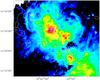 |
Fig. 1 Color image shows 70 μm continuum emission observed with PACS. The white contours represent 13CO (1–0) emission integrated between 68.9 and 70.3 km s-1 corresponding to the “filament”, observed using FCRAO as part of the Galactic Ring Survey. The black cross shows the position of the HIFI observations. |
As part of the Herschel key program “PRobing InterStellar Molecules with Absorption line Studies (PRISMAS) we have observed several selected spectral lines in absorption toward the source W51e2 to study the foreground material along the line of sight using HIFI. These observations have for the first time detected in absorption a component at 70 km s-1 (a velocity even higher than the velocity of the 68 km s-1 filament) along with the 57 km s-1 source velocity component, in C3, HDO, and NH3. The observation of C3 was motivated by the importance of small carbon chains for the chemistry of stellar and interstellar environments either as building blocks for the formation of long carbon chain molecules, or as are products of photo-fragmentation of larger species such as PAHs (Radi et al. 1988; Pety et al. 2005). C3 has been identified with Herschel/HIFI for the first time in the warm envelopes of star-forming hot cores like W31C, W49N and DR21(OH) (Mookerjea et al. 2010, 2012). Within the PRISMAS program, the ground-state HDO transition at 894 GHz has only been detected at the velocity of the H ii regions. Based on observations of high-mass star-forming regions (Jacq et al. 1990; Pardo et al. 2001; van der Tak et al. 2006; Persson et al. 2007; Bergin et al. 2010) and low-mass protostars (Liu et al. 2011; Coutens et al. 2012, 2013a), the HDO/H2O ratio remains lower than the D/H ratio derived for other deuterated molecules observed in the same sources although it is clearly higher than the cosmic D/H abundance. This low deuterium enrichment of water could provide an important constraint to the astrochemical models to explain the chemical processes involved in the formation of water. Ammonia (NH3) is a key species in the nitrogen chemistry and a valuable diagnostic because its complex energy level structure covers a very broad range of critical densities and temperatures. It has been observed throughout the ISM ever since its detection in 1968 (Cheung et al. 1968) but mainly in its inversion lines at cm wavelengths. With Herschel it became possible to observe ground-state rotational transitions with high critical densities at THz frequencies of both ortho and para symmetries, for instance, in cold envelopes of protostars (Hily-Blant et al. 2010), in diffuse/translucent interstellar gas (Persson et al. 2012), and hot cores (Neill et al. 2013).
We have combined the HIFI observations with IRAM observations of CCH, c-C3H2 and CN in all of which the 70 km s-1 feature is detected in absorption. We have used local thermodynamic equilibrium (LTE) and non-LTE models to derive the physical parameters of the dense clump at 70 km s-1 and its relation to the W51 molecular cloud. We also present a gas-grain, warm-up chemical model that consistently explains the abundances of all the species observed in the clump. This paper is organized as follows: Sects. 2 and 3 describe the Herschel and IRAM observations, respectively. Section 4 describes the complex velocity structure observed along the sightline to W51e2. Section 5 discusses the column and volume densities derived from all the tracers that detect the 70 km s-1 clump. In Sect. 6 we compare the observed abundances of the various chemical species with a grain warm-up based chemical model. Section 7 discusses various derived properties of the 70 km s-1 clump and presents a possible formation scenario for the clump.
2. Observations with Herschel/HIFI
Spectroscopic parameters for the observed spectral lines.
In the framework of the Herschel key program PRISMAS (P. I. M. Gerin), we observed the line of sight toward the compact H ii region W51e2, whose coordinates are α(J2000) = 19h23m43 90 δ(J2000) = 14°30′30.̋5. The observations were performed in the pointed dual-beam switch (DBS) mode using the HIFI instrument (de Graauw et al. 2010; Roelfsema et al. 2012) onboard Herschel (Pilbratt et al. 2010). The DBS reference positions were situated approximately 3′ east and west of the source. The HIFI Wide Band Spectrometer (WBS) was used with optimization of the continuum, providing a spectral resolution of 1.1 MHz over an instantaneous bandwidth of 4 × 1 GHz. To separate the lines of interest from the lines in the other sideband, which could possibly contaminate our observations, we observed the same transition with three different LO settings. This method is necessary in such chemically rich regions to ensure genuine identification of spectral lines. The data were processed using the standard HIFI pipeline up to level 2 with the ESA-supported package HIPE 8.0 (Ott 2010) and were then exported as FITS files into CLASS/GILDAS format2 for subsequent data reduction. Both polarizations were averaged to reduce the noise in the final spectrum. The baselines obtained and subtracted are well fitted by straight lines over the frequency range of the whole band. The single sideband continuum temperature derived from the polynomial fit at the line frequency was added back to the spectra.
We followed up the detection of the 70 km s-1 velocity component in C3 by searching for the feature in different available transitions of HDO, NH3, CCH, c-C3H2, and CN. Among these chosen molecules, c-C3H2 and CCH are chemically related to C3 since they are the by-products of the proposed formation route of C3 via warm-up of the CH4 mantle of the grains, which essentially refers to a temperature of 30 K and higher (Hassel et al. 2011). In contrast, NH3 and HDO are tracers of cold (20 K) and dense molecular gas. The abundance of CN is typically found to be low in hot cores, and higher in regions of intense UV fields such as the interfaces of H ii regions and molecular clouds.
2.1. Linear carbon chain, C3
We observed four transitions of the ν2 fundamental band, P(4), Q(2), Q(4), and P(10) of triatomic carbon using the bands 7a, 7b, and 6b of the HIFI receiver (Müller et al. 2005; Mookerjea et al. 2010). All spectroscopic information regarding the observed C3 lines is presented in Table 1. The observations were carried out on October 29, 2010 and April 22 and 23, 2011. Further details of the observations and data reduction are similar to the analysis of the W31C and W49N sources presented in Mookerjea et al. (2010). All spectra were smoothed to resolutions of between ~0.16 to 0.18 km s-1 and the rms noise level for the spectra ranges between 0.03 to 0.04 K (Fig. 2).
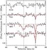 |
Fig. 2 HIFI observations of the C3 lines. The observed spectra (in black) are corrected for the DSB continuum and normalized to the SSB continuum level. Results of simultaneous fitting of P(4), Q(2) and Q(4) are shown in red. The observed spectrum of P(10) is also shown to illustrate the nondetection. |
2.2. NH3
We observed the ortho-NH3 2 –1
–1 and 1–0 ground-state transitions at 1214.8 (band 5a) and 572.5 GHz (band 1b) as well as the para-NH3 2
 –1
–1 ground transition at 1215.2 GHz (band 5a) (Yu et al. 2010). The beam size is ~37′′ for the low frequency transition and 17.5′′ for the higher frequencies transitions. The forward efficiency is 0.96 and the main beam efficiencies are 0.76 (at 572 GHz) and 0.64 (at 1215 GHz). The PRISMAS observations were carried out on October 29, 2010 and April 22, 2011. Additionally, we used the para-NH3 2–1 transition at 1168.45 GHz and 3
 –2
–2 transition at 1763.82 GHz observations obtained within the OT1 programme on absorption studies of N-hydrides. These observations were performed on April 18 and 21, 2012. Spectroscopic and observational details for all transitions are summarized in Table 1.
Observation parameters for CCH with PdBI.
2.3. HDO
We observed one of the HDO fundamental transitions (11,1–00,0) at 893.6 GHz (using the spectroscopic catalog JPL: Pickett et al. 1998) in band 3b. The beam is about 24.̋1 and the forward efficiency and the main beam efficiency are 0.96 and 0.74, respectively. The observations were carried out on October 27, 2010. Spectroscopic and observational details are summarized in Table 1.
3. Ground-based IRAM observations
3.1. CCH with PdBI
Plateau de Bure Interferometer (PdBI) observations dedicated to the PRISMAS project were carried out with six antennas in September 2007. The 4 GHz instantaneous IF–bandwidth allowed us to simultaneously observe CCH (plus six other lines) at 3 mm using seven different 40 MHz–wide correlator windows. One additional 320 MHz–wide correlator window was used to simultaneously measure the 3 mm continuum. The CCH line was detected in emission and absorption (spectroscopic details in Table 1).
We observed W51e2 in track-sharing mode in the D configuration (baseline lengths from 24 to 97 m). A two-fields Nyquist-sampled mosaic was needed to cover the W51e2 continuum emission. The D configuration was observed for about 7 h of telescope time. This leads to on–source integration time of useful data of 1.5 h for W51e2 after removing the bad data. The rms amplitude noise of the bandpass calibration was 0.5%. The rms phase noise were between 7 and 18°, which introduced position errors of <0.̋25. The typical resolution is 5.̋1 and the primary beam at the frequency of the CCH transition at 87.328585 GHz is 56.̋6. Table 2 presents the relevant parameters for these observations.
The data were reduced with the GILDAS software supported at IRAM (Pety 2005). Standard calibration methods using nearby calibrators were applied. The calibrators used for the absolute flux calibration are B1749+096 (5.2 Jy) and B1923+210 (1.4 Jy), respectively. The W51e2 data were processed using natural weighting to obtain the optimal signal-to-noise ratio. The line emission extension exceeds one third of the primary beam, implying the need for short-spacings from a single-dish telescope. However, we are interested here in the absorption lines in front of the continuum source, which is compact enough to avoid the need for short-spacings. The data were deconvolved using the Högbom CLEAN algorithm with a support defined around the continuum source to guide the search of the CLEAN components.
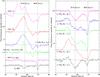 |
Fig. 3 Left: comparison of velocity structure seen in C3 spectra with that seen in transitions of CCH, c-C3H2, HDO, and CN. The H |
3.2. CN and c-C3H2 with IRAM 30 m
The CN J = 1–0 transition was observed at the IRAM-30 m telescope at Pico Veleta (Spain) in December 2006 in wobbler-switching mode and detected through its F = 1/2–1/2, 1/2–3/2, 3/2–1/2, 3/2–3/2 hyperfine components (see Table 1). All the details about these observations can be found in Godard et al. (2010). The CN J = 2–1 transition was also observed in parallel with J = 1–0 in its F = 5/2–3/2, 7/2–5/2, 3/2–1/2, 3/2–3/2, 5/2–5/2 and 3/2–5/2 hyperfine components (see Table 1), although this is not reported in Godard et al. (2010). The half-power beam width is about 22′′ at 113 GHz compared with the 11′′ value at 227 GHz.
The c–C3H2 21,2–10,1 transition at 85.3 GHz was observed in December 2006 (Gerin et al. 2011). The spectroscopic details are quoted in Table 1.
4. New velocity component along the W51e2 sightline
To determine the spatial distribution of gas in the W51e2 region, the velocity components originating in the local gas need to be separated from those produced by gas along the line of sight to the background continuum source. Fortunately, this source was observed in detail using several transitions of atomic and molecular species. For example, H109α observations toward W51e2 showed that the average velocity of the ionized gas is ≃56.8 km s-1(Wilson et al. 1970). Koo (1997) used H i observations toward W51e2 to identify two sets of absorption features, the local features at 6.2, 11.8 and 23.1 km s-1 and features proposed to be belonging to the Sagittarius spiral arm at 51.1, 62.3, and 68.8 km s-1. We note that for the H i observations the line widths range between 7.1 and 12.2 km s-1 with a spectral resolution of 2.1 km s-1, thus leading to an uncertainty in the velocity determination. However, the highest velocity permitted by Galactic rotation is about 60 km s-1 in this direction. Therefore the 62.3 and 68.8 km s-1 components are most likely associated with a high-velocity (HV) stream. Note also that the CO line emission is brightest at vLSR = 58 km s-1 (Kang et al. 2010), indicating that the ionized and molecular gas have similar velocities and are probably associated with the same radio continuum source.
Using H2CO observations, Arnal & Goss (1985) detected five absorption components at ~52, 55, 57, 66, and 70 km s-1 toward W51e2. As discussed above, the 57 km s-1 component seems to be associated with the H ii region. The 62 km s-1 component detected in H i and not in H2CO is understood to be a H i cloud associated with W51e2 (G49.5-0.4). H2CO absorption between 66 and 70 km s-1 and HI absorption at 68.8 km s-1 imply that the HV stream is in front of W51e. In the large-scale 12CO and 13CO channel maps, the emission feature in the 66 to 70 km s-1 velocity range traces a filamentary structure that extends across a region ~1° in size that contains most of the H ii regions associated with W51. This is consistent with the triggered star formation scenario that is due to the interaction of the filament with the main cloud, as proposed by Carpenter & Sanders (1998). Recently, Kang et al. (2010) compared the molecular cloud morphology with the distribution of IR and radio continuum sources and found associations between molecular clouds and young stellar objects listed in Spitzer IR catalogs. Star formation in the W51 complex appears to have occurred in a long and large filament along with the H ii regions. Young stellar objects along the filament are younger and more massive than those in the surrounding regions (Carpenter & Sanders 1998). Cloud-cloud collisions may compress the interface region between two colliding clouds and initiate star formation. The molecular clouds at this interface are heated, but the molecular clouds on the trailing side remain cold. The diffuse emission from the giant molecular cloud truncates at the location of the 68 km s-1 cloud for velocities higher than 63 km s-1. The W51 cloud and filament are probably at a common distance since such an interface is unlikely to result from the chance superposition of unrelated molecular clouds.
Basic observational results for NH3, HDO, CCH, and c-C3H2.
Figure 2 shows the observed C3 spectra normalized to the (single-sideband) continuum level. We identify two major absorption dips around 58 and 70 km s-1 in the spectra of all three transitions of C3. Figure 3 shows the observed spectra of single or multiple transitions of CCH, c-C3H2, NH3, CN, HDO, and H O along with the C3 (Q(2)) spectrum for comparison. The HO 11,1–00,0 spectrum was observed with Herschel/HIFI as part of the PRISMAS program and has been presented by Flagey et al. (2013).
While the 58 km s-1 component appears either in emission or in absorption, depending on the transitions, the narrow 70 km s-1 feature can be seen only as a deep absorption feature for the different species presented here. The absorption dip at 58 km s-1 is broad and most likely is a combination of the 57 km s-1 component associated with the H ii region W51e2 and the H i cloud at 62 km s-1. We note that although the 68 km s-1 feature associated with the filament has been relatively easily detected in CO emission (Mufson & Liszt 1979; Carpenter & Sanders 1998), the line profiles are much broader than the 70 km s-1 absorption dip detected here. Based on the results of our analyses we show in the following sections that the 70 km s-1 absorption feature can only be explained in terms of a high-density (>105 cm-3) clump that formed within the filament.
5. Estimations of the column and volume densities
Tables 3 and 4 summarize the basic observational results for CCH, c-C3H2, NH3, HDO, and C3. The central velocities, linewidths, and main-beam temperatures of all species are derived by fitting Gaussian components to the 70 km s-1 feature of the observed spectra. In the following analyses, we assumed that the foreground cloud at 70 km s-1 completely fills the beam.
5.1. C3 LTE modeling
We fitted the three detected transitions of C3 simultaneously using two Gaussian components corresponding to two velocity components per transition. The fit derives a common vLSR and full width at half maximum (Δv) for each of the velocity components for all transitions as well as the strength of the absorption dips. Table 4 presents the single-sideband continuum levels (estimated from double-sideband temperatures assuming a sideband gain ratio of unity) and the opacities derived from the Gaussian fitting.
Assuming LTE we used the level-specific column densities derived from the C3 absorption dips (Table 4) following the rotation diagram method. For the 58 km s-1 component we estimate the rotation temperatures (Trot) and total column density (N(C3)) to be 10 K and 1.0 × 1014 cm-2, respectively, for the 70 km s-1 component these are 10 K and 6.0 × 1013 cm-2, respectively. Since the determination of Trot and the column density involves fitting of only two datapoints with associated uncertainties to estimate two parameters, the derived parameters are expected to have very large uncertainties. Additionally, since the far-infrared continuum radiation is known to contribute significantly to the excitation of C3 (Roueff et al. 2002), an accurate estimate of temperature can only be obtained using rigorous radiative transfer treatment. We therefore only used the derived total column densities from the LTE analysis.
5.2. Column density estimates from LTE modeling: CCH and c-C3H2
We used the IRAM-30 m c-C3H2 observations presented by Gerin et al. (2011) and the IRAM-PdBI CCH observations to compute the column densities in the absorption components along the line of sight to W51e2 using the CASSIS software3.
Derived parameters for the absorption components detected in CCH and c-C3H2 spectra.
For CCH we used the average (taken over 5′′) spectrum centered on the HIFI position observed with PdBI for modeling. We detected the 70 km s-1 absorption feature in only one transition of each of CCH and c-C3H2. Since both CCH and c-C3H2 lines at 70 km s-1 appear in emission instead of absorption for Tex> 3 K, we derived the molecular column densities for each velocity component in absorption assuming that the excitation temperature equals the CMB. The ratio of the column densities of CCH and c-C3H2 in the 70 km s-1 component (~67) is similar to the value found in the extended ridge component (N(H2) = 3 × 1023 cm-2) of the OMC-1 region (Blake et al. 1987, see Sect. 7.1).
5.3. Volume density estimates from NH3
Non-LTE (RADEX) modeling of NH3 and CN.
Because the ortho-NH3 fundamental transition at 572.5 GHz are highly optically thick, with blending in the line of sight (see Fig. 3), the 1168.5, 1214.8, 1215.2, and 1763.8 GHz transitions were used to separate the different components and extract the 69.2 ± 0.2 km s-1 component. The results from the Gaussian fitting procedure are presented in Table 3. Indeed, the 572 GHz transition is affected by blending and saturation effects and does not allow us to obtain a reliable estimate for the ortho-to-para ratio in the 70 km s-1 cloud, in addition to n(H2) and Tkin. Furthermore, we do not have additional observations that might be used to identify the NH3 formation process (temperature and mechanism in particular) (Persson et al. 2012) and the H2 ortho-para ratio (Faure et al. 2013), both of which are known to result in an NH3 ortho-para ratio significantly different from unity. We assumed the ortho-to-para ratio to be equal to the statistical equilibrium value of unity. The ortho- and para-NH3 collisional coefficients with para-H2 (Danby et al. 1988) were used in the non-LTE RADEX computations within CASSIS. In the CASSIS database the ortho and para separation is provided with partition functions for temperatures between 3 and 300 K. Note that there is a discrepancy between the fitted line widths of the two 21–11 (~3 km s-1) transitions and the 2–1 and 3–2 (2.0 km s-1) transitions. However, we argue that the line widths of the 21–11 transitions are more affected by additional components in its wings than the more isolated velocity components of the 3–2 and 2–1 transitions. We therefore varied the line width around a value of 2 km s-1 in the modeling. The best-fitting model for the 70 km s-1 cloud is obtained for a line width of 2 km s-1 with an H2 density of 5 × 105 cm-3, and a kinetic temperature of ~30 K, with a column density of 4.2 × 1013 cm-2 for each symmetry. Hence the total estimated column density of NH3 is 8.4 × 1013 cm-2.
5.4. Volume density estimates from CN
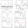 |
Fig. 4 Top panels: observed spectra of CN 1–0 (left) and CN 2–1 (right) shown in black. We also show the best-fit LTE model (using the CASSIS software) corresponding to Tex = 3 K, vLSR= 69.5 km s-1, Δv = 0.6 km s-1, and NCN = 5.8×1013 cm-2. The data and the relevant best-fit model spectra are enlarged in the four panels below. The details of the CN(1–0) transitions are middle row left: 1, 1/2, 1/2–0, 1/2, 3/2 and right: 1, 1/2, 3/2–0, 1/2, 1/2; bottom row left: 1, 1/2, 3/2–0, 1/2, 3/2. |
We observed the J = 1–0 and 2–1 transitions of CN using the IRAM 30 m. CN 1–0 is a four component multiplet that appears in absorption against the 0.95 K continuum, and CN 2–1 is a six component multiplet, four components of which appear in absorption against the 2.1 K continuum (the other components are blended with the emission components at the source velocity). Figure 4 shows the observed spectra along with the best-fit LTE model for Tex = 3 K, vLSR = 69.5 km s-1, line width of 0.6 km s-1 and a total column density of 5.8 × 1013 cm-2. Recently, the collision rates have been computed with p-H2 taking into account all the CN hyperfine levels (Kalugina et al. 2012). Assuming the line width of the 70 km s-1 component to be 0.6 km s-1, we ran a non-LTE model (RADEX) to reproduce the seven CN hyperfine components seen in absorption and found a density of n(H2) ~ 105 cm-3 (assuming that H2 is mainly in its para form) and a kinetic temperature of ~6 K with a column density of ~5.5 × 1013 cm-2. Both the density and temperature required to explain the observed CN spectra are lower than the values required to explain the observed ammonia transitions (see Table 6). A possible reason for the low temperature derived can be the dilution of the continuum within the beam, combined with a cold foreground component that is covering part of the continuum. Assuming a higher continuum value (e.g. 1.7 K, as found for CCH) would lead to a 10 K kinetic temperature for the 70 km s-1 component. We therefore consider 6 K to be a lower limit for the temperature derived from CN. However, given the significantly different temperatures (30 K) and densities (5 × 105 cm-3) found for NH3 along with the extremely narrow line width of the CN lines compared with those found in NH3, C3, and HDO, it is very likely that CN arises from a colder and less dense envelope, possibly giving rise to CCH and c-C3H2 as well.
Abundances of all chemical species estimated relative to the observed CCH column density in the 70 km s-1 clump.
5.5. HDO
Most of the compact H ii regions observed within the PRISMAS key program present a broad absorption profile in the 893 GHz fundamental transition of HDO at the source vLSR. The W51 region is the only high-mass source where this transition appears as a deep narrow (<2 km s-1) feature at a velocity higher than the source velocity. The other HDO fundamental transition at 464 GHz has also been observed but the high-velocity absorption feature is not detected reliably above the noise of the spectrum (rms = 0.13 K). From the narrow component observed at 893 GHz, we can state that this component is clearly localized and probably not extended along the line of sight. Both HDO ground-state transitions have high critical densities (>107 cm-3) and do not provide strong constraints on the kinetic temperature or density for the range found with the NH3 and CN analysis. Because the NH3 transitions trace a dense region in the filament, which is also more likely to emit in HDO than the lower density and lower temperature region that is traced by CN, we estimate for Tkin = 30 K and n(H2) = 5 × 105 cm-3 the total HDO column density under non-LTE to be 1.5 × 1012 cm-2, which is similar to the LTE value with an excitation temperature of 3 K.
6. Chemical modeling of abundance
In the absence of a direct estimate for the H2 column density for the 70 km s-1 clump, we expressed the abundances of all the observed molecules C3, c-C3H2, NH3, CN, and HDO (Table 7) relative to the column density of CCH and compared this with the results of the Ohio State University (OSU) gas-grain chemical model with a warm-up (Hasegawa et al. 1992; Garrod & Herbst 2006). A previous version of this model has already been used to interpret the abundance of C3 in the warm envelopes of hot cores such as W31C, W49N, and DR21OH (Mookerjea et al. 2010, 2012). While the 70 km s-1 component is not directly associated to the hot core, the necessity of grain warm-up in explaining the abundance of C3 in dense environments was illustrated by Hassel et al. (2011). As explained by Mookerjea et al. (2012), formation of C3 in dense environments cannot proceed via the gas-phase pathway as in diffuse clouds and requires desorption (either by radiation or by cosmic ray) of CH4 from icy grain mantles to produce C2H2, which reacts further to produce C3.
The chemical model is adapted from models of the hot-core phase of protostellar sources (Viti et al. 2004; Garrod & Herbst 2006). Standard hot-core chemistry requires that dust grains build up icy mantles at early times, when the temperature is low (~10 K) and the core is in a state of collapse (Brown et al. 1988). Later, the formation of a nearby protostar quickly warms the gas and dust (warm-up phase), re-injecting the grain mantle material into the gas phase, and stimulating a rich chemistry. Thus, hot-core models can involve three distinct phases: (i) the collapse of a cold clump of interstellar gas to high densities; (ii) heating of this clump, and the subsequent evaporation of grain mantles; and (iii) the hot-core phase. The present model examines (ii), the warm-up phase, and starts from the time at which the clump has collapsed to the high density and considers heating of the constant density clump and subsequent grain surface and gas-phase chemistry, corresponding to Phase 2 of Viti et al. (2004), based on the approximation of Hassel et al. (2008). In the warm-up approach, a one-point parcel of material undergoes an initially cold period of T0 = 10 K with a duration of t = 105 yr, followed by a gradual temperature increase to a maximum temperature, Tmax. A heating time-scale of th = 0.2 Myr was adopted following Garrod & Herbst (2006), in which the temperature reaches Tmax by 0.3 Myr. In the warm-up, the dust and gas temperatures are assumed to be equal and follow the same evolution. Unlike the hot-core models, it is unclear whether the filament harbors star formation. We therefore considered values of Tmax that represent relatively mild warming. The physical parameters adopted are the same as used by Garrod et al. (2007) and Hassel et al. (Table 1; 2008), including a canonical value for cosmic-ray ionization rate ζ = 1.3 × 10⁻¹⁷ s-1. The simplified warm-up and the estimates for the parameters were previously adopted by Hassel et al. (2008) following Garrod & Herbst (2006) to investigate the details of chemical evolution without a strict dependence on a particular dynamical model, and have since been used in Hassel et al. (2011) and Mookerjea et al. (2012). Although the dense clump may not contain a hot core, we adopted the same approach in this model for the same general reason, and in particular to incorporate reactions involving D-bearing species into a familiar modeling procedure.
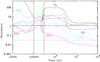 |
Fig. 5 Calculated abundances of different species relative to the observed column density of CCH, as a function of time for a constant density n(H2) = 5 × 105 cm-3 and a warm-up to Tmax = 30 K from 10 K, where the warm-up and other conditions are described in Sect. 6. The dashed horizontal lines correspond to the observed abundances and are color-coded with the calculated abundances. The vertical lines at t = 0.1 and 0.3 Myr indicate the onset and end of warm-up of grains, respectively. |
The gas-grain chemistry reaction network has been expanded since the previous C3 models to include HDO, and now comprises 7882 reactions involving 735 gaseous and surface species. We included the major gaseous D-exchange reactions of the UMIST database (McElroy et al. 2013), the major surface reactions identified by Stantcheva & Herbst (2003), and gas-phase reactions related to HDO using the approach of Aikawa et al. (2012). The initial chemical abundances were adopted from Garrod et al. (2007), and include the initial abundance [HD] = 1.5 × 10⁻⁵ × [H2] (Osamura et al. 2005).
The observed multiple transitions of NH3 provide the only independent estimate of the density and temperature of the filament that gives rise to the 70 km s-1 component. Here we present a comparison of the observed abundances for all molecules considered with the abundances predicted by the chemical model for which Tmax is 30 K and the molecular hydrogen density is 5 × 105 cm-3 (Fig. 5). The predicted abundances of all molecules are significantly different from the observed values at times earlier than ~3 Myr. The abundances of NH3, CCH, and CN predicted by the model match the observed abundances well at all times beyond t = 3.5 Myr. The model abundance of c-C3H2, is significantly higher than the observed abundance, at all times. Previous models using a similar chemical network have also demonstrated a larger calculated abundance than the observation (Fig. 4; Hassel et al. 2011). It is also possible that c-C3H2 arises in a colder and less dense envelope (similar to CN), than the values of n(H2) and Tmax used in the model presented here. Beyond 5 Myr the model abundance of C3 approaches the observed abundance for all times up to t = 70 Myr. For C3 the model abundance is within a factor of 3 of the observed abundance for all times later than 5 Myr. The HDO model abundance is consistent to within a factor of 2.5 of the observed abundance between 3.5 to 30 Myr and diverges farther at later times.
7. Discussion
In the direction of W51e2 we have for the first time detected HDO and C3 in a dense molecular clump at 70 km s-1 that is not directly associated with hot star-forming cores.
C3 in dense clouds has so far only been detected in the warm envelopes associated with star-forming cores. Abundance of C3 in dense clouds is explained via warming-up of grain mantles to release CH4 and subsequently C3H2, the first step in the chemical pathway for the formation of C3, as explained in detail in Hassel et al. (2011) and Mookerjea et al. (2012). Thus, detection of C3 in the dense clump at 70 km s-1 otherwise not identified as a star-forming region is as surprising as the detection of deuterated water in the cloud that is physically not related to the W51 region. HDO is most likely formed in the ice mantles within cold (<20 K) translucent clouds (Cazaux et al. 2011) in regions shielded from UV radiation. Indeed, at Av ≳ 3 (Whittet et al. 1988), species from the gas phase accrete onto dust grains and initiate ice formation. After the formation of water and deuterated water in the ice mantles in the star formation scenario, the environment undergoes gravitational collapse and the local density increases, leading to the formation of a protostar. The surrounding medium then heats up and releases the icy mantles into the gas phase, leading to a significant HDO abundance in the gas phase (Coutens et al. 2012, 2013b). Based on the non-LTE modeling of the five observed NH3 transitions, we characterize the region of the filament that gives rise to the 70 km s-1 feature as having Tkin = 30 K and n(H2) = 5 ×105 cm-3. The abundances predicted by the grain warm-up chemical model reproduce the observed abundances to within factors of 2 to 3 at all times later than 3.5 Myr for all species except for c-C3H2.
7.1. CCH/c-C3H2 ratio in the clump
Previous observations of CCH and c-C3H2 toward dense dark clouds and Photon Dominated Regions (PDRs) derived a tight correlation between the two species. The ratio N(CCH)/ N(c-C3H2) is ~61 in OMC-1 (Blake et al. 1987) and it ranges between 10 and 25 in PDRs such as Horsehead nebula and IC63 whereas in dark clouds such as TMC-1, and L134N the ratio is ~1 (Teyssier et al. 2004). For the dense clump detected toward W51e2 the observed N(CCH)/N(c-C3H2) of 67 is closer to the value observed in the dense active star-forming region OMC-1 than to the values seen in UV-illuminated clouds and dark clouds.
7.2. Deuterium enrichment in the clump
Using Herschel/HIFI, a number of transitions of H2O and H218O species corresponding to a range of excitations have been observed for the first time. The 70 km s-1 feature is detected unambiguously in the H2O 20,2–11,1 transition as well as the H218O 11,1–00,0 transition (Flagey et al. 2013). However, an accurate determination of the total H2O column density is compromised by the crowded environment along the line of sight with high optical depth, as well as by partial blending of the components. The column density for the less abundant para-H218O species is estimated to be (7 ± 1) 1011 cm-2 for the 70 km s-1. The abundance ratio between 16O and 18O is commonly accepted to be ~560 (Wilson & Rood 1994), although significant variation has been observed throughout the Galaxy. Accordingly, we estimate a D/H ratio in water vapor of about 9.6 × 10⁻⁴ (assuming an ortho-para ratio of 3), similar to the value found in Orion KL by Neill et al. (2013). This ratio has also been estimated from HDO observations of the low-mass protostar IRAS 16293-2422 (Coutens et al. 2012, 2013a). The derived values of HDO/H2O were 1.8 × 10⁻² in the hot core, 5 × 10⁻³ in the cold envelope, and about 4.8 × 10⁻² in the external photodesorption layer. The value estimated from our analysis is consistent with the value found in the cold envelope of the IRAS 16293-2422 low-mass star-forming region, in which the ices are not affected by thermal desorption or photo-desorption by the FUV field. For the best-fit grain warm-up model that reproduces the observed abundances of the other molecules, at times later than 3.5 Myr the HDO/H2O ratio drops from 0.002 to 0.001 for an initial HD/H2 ratio of 1.5 × 10⁻⁵. The calculated HDO/H2O ratio is consistent with the observed ratio of 9.6 × 10⁻⁴. Although HDO forms in the medium density, pre-collapse phase, it mostly remains on grain mantles, since the nonthermal desorption mechanisms have a limited efficiency. In these models, which reach only 30 K, the release of HDO into the gas phase is attributed to nonthermal processes related to cosmic-ray interactions rather than warming up or direct FUV photodesorption. Although the chemical model predicts an HDO/H2O ratio consistent with the observed value for t> 3.5 Myr, it overestimates the HDO/H2O ratio by more than a factor of 10 for earlier times t< 1 Myr. The calculated HDO/H2O ratio is substantially enriched above the initial HD/H2 ratio, primarily because of the grain surface formation route of HDO. The ratio is furthermore enriched above the observed value because of the lower column density of H2O calculated by the chemical models. We explored the possibility of enhanced cosmic-ray ionization rates. For enhanced cosmic ray rates the chemical models produce abundances very different from the observed values for all molecules. This result for the 70 km s-1 cloud is in contrast to the higher values of ζ deduced by Indriolo et al. (2012) along the same line of sight for the absorption features arising because of diffuse foreground. This implies that the absorbing gas is not diffuse, but is dense with a standard value of ζ.
7.3. Possible origin of the clump
The 70 km s-1 absorption dip caused by the foreground material in the direction of W51e2, although not associated with a star-forming core, shows chemical abundances typically found in the envelopes of low-mass protostellar candidates. We propose that the feature arises in a dense (n(H2) = (1–5) ×105 cm-3) and cold (10–30 K) clump that is formed within the much larger scale filament (detected in CO) deemed to be interacting with the W51 main molecular cloud. A possible scenario for the formation of the dense clump can be outlined based on the collision of the filament with W51 main (Kang et al. 2010). In this scenario, cloud-cloud collision lead to the compression of the interface region and initiate the formation of stars as seen in W51 (Habe & Ohta 1992). The molecular clumps at the interface are heated, but the molecular clumps on the trailing side remain cold and hence appear in absorption. Models for collision between two different clouds suggest that such collisions disrupt the larger cloud while the small cloud is compressed and subsequently forms stars. It is possible that the dense clump detected in absorption is formed on the trailing side of the filament that interacts with the main molecular cloud. Based on its density and somewhat elevated temperatures (~30 K), it is also possible that this cloud is also collapsing to eventually form stars. In the absence of any observational evidence, we currently do not consider the source to be an IRDC. We suggest that the nondetection of this star-forming clump in the continuum is due to its chance coincidence along the line of sight with the much stronger W51e2 continuum source.
Higher spectral and angular resolution observations of the foreground gas responsible for the absorption dip at ~70 km s-1 are needed to understand its spatial distribution. We also propose to explore a clearer detection of the protostar using mid-infrared observations of the strong spectral features of molecular ices toward this region.
The PACS data shown in Fig. 1 are a Level 2 data product produced by the standard data reduction pipeline for PACS-SPIRE parallel mode observations as obtained from the Herschel Science Archive. The 13CO data have taken from the Galactic Ring Survey done by FCRAO available online at http://www.bu.edu/galacticring/
See http://www.iram.fr/IRAMFR/GILDAS for more information about the GILDAS software.
A software developed by IRAP-UPS-CNRS: http://cassis.irap.omp.eu
Acknowledgments
We thank the anonymous referee for the suggestions that helped improve the clarity of the paper significantly. HIFI has been designed and built by a consortium of institutes and university departments from across Europe, Canada and the United States under the leadership of SRON Netherlands Institute for Space Research, Groningen, The Netherlands and with major contributions from Germany, France and the US. Consortium members are: Canada: CSA, U. Waterloo; France: CESR, LAB, LERMA, IRAM; Germany: KOSMA, MPIfR, MPS; Ireland, NUI Maynooth; Italy: ASI, IFSI-INAF, Osservatorio Astrofisico di Arcetri-INAF; Netherlands: SRON, TUD; Poland: CAMK, CBK; Spain: Observatorio Astronómico Nacional (IGN), Centro de Astrobiologá (CSIC-INTA). Sweden: Chalmers University of Technology – MC2, RSS & GARD; Onsala Space Observatory; Swedish National Space Board, Stockholm University – Stockholm Observatory; Switzerland: ETH Zurich, FHNW; USA: Caltech, JPL, NHSC. G. Hassel gratefully acknowledges helpful discussions and rate information provided by Yuri Aikawa. C. Vastel is grateful to F. Lique for providing the CN collisional rates in the LAMDA database format. T. Harrison thanks the Summer Scholars grant from the Center for Undergraduate Research and Creative Activity (CURCA), Siena College. This paper has made extensive use of the SIMBAD database, operated at CDS, Strasbourg, France. This publication makes use of molecular line data from the Boston University-FCRAO Galactic Ring Survey (GRS). The GRS is a joint project of Boston University and Five College Radio Astronomy Observatory, funded by the National Science Foundation under grants AST-9800334, AST-0098562, AST-0100793, AST-0228993, & AST-0507657. This paper is partly based on observations obtained with the IRAM Plateau de Bure interferometer and 30 m telescope. We are grateful to the IRAM staff at Plateau de Bure, Grenoble for their support during the observations and data reductions. IRAM is supported by INSU/CNRS (France), MPG (Germany), and IGN (Spain). Part of the research was carried out at the Jet Propulsion Laboratory, California Institute of Technology, under a contract with the National Aeronautics and Space Administration.
References
- Aikawa, Y., Wakelam, V., Hersant, F., Garrod, R. T., & Herbst, E. 2012, ApJ, 760, 40 [NASA ADS] [CrossRef] [Google Scholar]
- André, P., Men’shchikov, A., Bontemps, S., et al. 2010, A&A, 518, L102 [NASA ADS] [CrossRef] [EDP Sciences] [Google Scholar]
- Arnal, E. M., & Goss, W. M. 1985, A&A, 145, 369 [NASA ADS] [Google Scholar]
- Bally, J., Lanber, W. D., Stark, A. A., & Wilson, R. W. 1987, ApJ, 312, L45 [NASA ADS] [CrossRef] [Google Scholar]
- Bergin, E. A., Hogerheijde, M. R., Brinch, C., et al. 2010, A&A, 521, L33 [NASA ADS] [CrossRef] [EDP Sciences] [Google Scholar]
- Bieging, J. 1975, in H II Regions and Related Topics, eds. T. L. Wilson, & D. Downes (Berlin: Springer), Lect. Notes Phys., 42, 443 [Google Scholar]
- Blake, G. A., Sutton, E. C., Masson, C. R., & Phillips, T. G. 1987, ApJ, 315, 621 [NASA ADS] [CrossRef] [Google Scholar]
- Brown, P. D., Charnley, S. B., & Millar, T. J. 1988, MNRAS, 231, 40 [Google Scholar]
- Carpenter, J. M., & Sanders, D. B. 1998, AJ, 116, 1856 [NASA ADS] [CrossRef] [Google Scholar]
- Cazaux, S., Caselli, P., & Spaans, M. 2011, ApJ, 741, L34 [NASA ADS] [CrossRef] [Google Scholar]
- Cheung, A. C., Rank, D. M., Townes, C. H., Thornton, D. D., & Welch, W. J. 1968, Phys. Rev. Lett., 21, 1701 [Google Scholar]
- Coutens, A., Vastel, C., Caux, E., et al. 2012, A&A, 539, A132 [NASA ADS] [CrossRef] [EDP Sciences] [Google Scholar]
- Coutens, A., Vastel, C., Cazaux, S., et al. 2013a, A&A, 553, A75 [NASA ADS] [CrossRef] [EDP Sciences] [Google Scholar]
- Coutens, A., Vastel, C., Cabrit, S., et al. 2013b, A&A, 560, A39 [NASA ADS] [CrossRef] [EDP Sciences] [Google Scholar]
- Danby, G., Flower, D. R., Valiron, P., Schilke, P., & Walmsley, C. M. 1988, MNRAS, 235, 229 [NASA ADS] [CrossRef] [Google Scholar]
- de Graauw, T., Helmich, F. P., Phillips, T. G., et al. 2010, A&A, 518, L6 [NASA ADS] [CrossRef] [EDP Sciences] [Google Scholar]
- Faure, A., Hily-Blant, P., Le Gal, R., Rist, C., & Pineau des Forêts, G. 2013, ApJ, 770, L2 [NASA ADS] [CrossRef] [Google Scholar]
- Flagey, N., Goldsmith, P. F., Lis, D. C., et al. 2013, ApJ, 762, 11 [NASA ADS] [CrossRef] [Google Scholar]
- Garrod, R. T., & Herbst, E. 2006, A&A, 457, 927 [NASA ADS] [CrossRef] [EDP Sciences] [Google Scholar]
- Garrod, R. T., Wakelam, V., & Herbst, E. 2007, A&A, 467, 1103 [NASA ADS] [CrossRef] [EDP Sciences] [Google Scholar]
- Gaume, R. A., Johnston, K. J., & Wilson, T. L. 1993, ApJ, 417, 645 [NASA ADS] [CrossRef] [Google Scholar]
- Gerin, M., Kaźmierczak, M., Jastrzebska, M., et al. 2011, A&A, 525, A116 [NASA ADS] [CrossRef] [EDP Sciences] [Google Scholar]
- Godard, B., Falgarone, E., Gerin, M., Hily-Blant, P., & de Luca, M. 2010, A&A, 520, A20 [NASA ADS] [CrossRef] [EDP Sciences] [Google Scholar]
- Habe, A., & Ohta, K. 1992, PASJ, 44, 203 [NASA ADS] [Google Scholar]
- Hasegawa, T. I., Herbst, E., & Leung, C. M. 1992, ApJS, 82, 167 [NASA ADS] [CrossRef] [Google Scholar]
- Hassel, G. E., Herbst, E., & Garrod, R. T. 2008, ApJ, 681, 1385 [NASA ADS] [CrossRef] [Google Scholar]
- Hassel, G. E., Harada, N., & Herbst, E. 2011, ApJ, 743, 182 [NASA ADS] [CrossRef] [Google Scholar]
- Hily-Blant, P., Maret, S., Bacmann, A., et al. 2010, A&A, 521, L52 [NASA ADS] [CrossRef] [EDP Sciences] [Google Scholar]
- Indriolo, N., Neufeld, D. A., Gerin, M., et al. 2012, ApJ, 758, 83 [NASA ADS] [CrossRef] [Google Scholar]
- Jacq, T., Walmsley, C. M., Henkel, C., et al. 1990, A&A, 228, 447 [NASA ADS] [Google Scholar]
- Kalugina, Y., Lique, F., & Klos, J. 2012, MNRAS, 422, 812 [NASA ADS] [CrossRef] [Google Scholar]
- Kang, M., Bieging, J. H., Kulesa, C. A., et al. 2010, ApJS, 190, 58 [NASA ADS] [CrossRef] [Google Scholar]
- Koo, B.-C. 1997, ApJS, 108, 489 [NASA ADS] [CrossRef] [Google Scholar]
- Lique, F. 2010, J. Chem. Phys. 132, 044311 [Google Scholar]
- Liu, F.-C., Parise, B., Kristensen, L., et al. 2011, A&A, 527, A19 [NASA ADS] [CrossRef] [EDP Sciences] [Google Scholar]
- Low, F. J., Young, E., Beintema, D. A., et al. 1984, ApJ, 278, L19 [NASA ADS] [CrossRef] [Google Scholar]
- Lucas, R., & Liszt, H. S. 2000, A&A, 358, 1069 [NASA ADS] [Google Scholar]
- McElroy, D., Walsh, C., Markwick, A. J., et al. 2013, A&A, 550, A36 [NASA ADS] [CrossRef] [EDP Sciences] [Google Scholar]
- Mehringer, D. M. 1994, ApJS, 91, 713 [NASA ADS] [CrossRef] [Google Scholar]
- Molinari, S., Swinyard, B., Bally, J., et al. 2010a, A&A, 518, L100 [NASA ADS] [CrossRef] [EDP Sciences] [Google Scholar]
- Molinari, S., Abergel, A., Rivera-Ingraham, A., et al. 2010b, 38th COSPAR Scientific Assembly, Bremen, Germany [Google Scholar]
- Mookerjea, B., Giesen, T., Stutzki, J., et al. 2010, A&A, 521, L13 [NASA ADS] [CrossRef] [EDP Sciences] [Google Scholar]
- Mookerjea, B., Hassel, G. E., Gerin, M., et al. 2012, A&A, 546, A75 [NASA ADS] [CrossRef] [EDP Sciences] [Google Scholar]
- Mufson, S. L., & Liszt, H. S. 1979, ApJ, 232, 451 [NASA ADS] [CrossRef] [Google Scholar]
- Müller, H. S. P., Schlöder, F., Stutzki, J., & Winnewisser, G. 2005, J. Mol. Struct., 742, 215 [NASA ADS] [CrossRef] [Google Scholar]
- Neill, J. L., Wang, S., Bergin, E. A., et al. 2013, ApJ, 770, 142 [NASA ADS] [CrossRef] [Google Scholar]
- Osamura, Y., Roberts, H., & Herbst, E. 2005, ApJ, 621, 348 [NASA ADS] [CrossRef] [Google Scholar]
- Ostriker, J. 1964, ApJ, 140, 1056 [NASA ADS] [CrossRef] [MathSciNet] [Google Scholar]
- Ott, S. 2010, Astronomical Data Analysis Software and Systems XIX, ASP Conf. Ser., 434, 139 [NASA ADS] [Google Scholar]
- Pardo, J. R., Cernicharo, J., Herpin, F., et al. 2001, ApJ, 562, 799 [NASA ADS] [CrossRef] [Google Scholar]
- Persson, C. M., Olofsson, A. O. H., Koning, N., et al. 2007, A&A, 476, 807 [NASA ADS] [CrossRef] [EDP Sciences] [Google Scholar]
- Persson, C. M., Black, J. H., Cernicharo, J., et al. 2010, A&A, 521, L45 [NASA ADS] [CrossRef] [EDP Sciences] [Google Scholar]
- Persson, C. M., De Luca, M., Mookerjea, B., et al. 2012, A&A, 543, A145 [NASA ADS] [CrossRef] [EDP Sciences] [Google Scholar]
- Pety, J. 2005, SF2A-2005: Semaine de l’Astrophysique Française, eds. F. Casoli, T. Contini, J. M. Hameury, & L. Pagani (EDP Sciences), 721 [Google Scholar]
- Pety, J., Teyssier, D., Fossé, D., Gerin, M., et al. 2005, A&A, 435, 885 [NASA ADS] [CrossRef] [EDP Sciences] [Google Scholar]
- Pickett, H. M., Poynter, R. L., Cohen, E. A., et al. 1998, J. Quant. Spectr. Rad. Transf., 60, 883 [NASA ADS] [CrossRef] [Google Scholar]
- Pilbratt, G. L., Riedinger, J. R., Passvogel, T., et al. 2010, A&A, 518, L1 [CrossRef] [EDP Sciences] [Google Scholar]
- Radi, P. P., Bunn, T. L., Kemper, P. R., Molchan, M. E., & Bowers, M. T. 1988, J. Chem. Phys., 88, 2809 [NASA ADS] [CrossRef] [Google Scholar]
- Roelfsema, P. R., Helmich, F. P., Teyssier, D., et al. 2012, A&A, 537, A17 [NASA ADS] [CrossRef] [EDP Sciences] [Google Scholar]
- Roueff, E., Felenbok, P., Black, J. H., & Gry, C. 2002, A&A, 384, 629 [NASA ADS] [CrossRef] [EDP Sciences] [Google Scholar]
- Sato, M., Reid, M. J., Brunthaler, A., & Menten, K. M. 2010, ApJ, 720, 1055 [NASA ADS] [CrossRef] [Google Scholar]
- Scott, P. F. 1978, MNRAS, 183, 435 [NASA ADS] [Google Scholar]
- Stantcheva, T., & Herbst, E. 2003, MNRAS, 340, 983 [NASA ADS] [CrossRef] [Google Scholar]
- Teyssier, D., Fossé, D., Gerin, M., et al. 2004, A&A, 417, 135 [NASA ADS] [CrossRef] [EDP Sciences] [Google Scholar]
- Ungerechts, H., & Thaddeus, P. 1987, ApJS, 63, 645 [NASA ADS] [CrossRef] [Google Scholar]
- van der Tak, F. F. S., Walmsley, C. M., Herpin, F., & Ceccarelli, C. 2006, A&A, 447, 1011 [NASA ADS] [CrossRef] [EDP Sciences] [Google Scholar]
- Viti, S., Collings, M. P., Dever, J. W., et al. 2004, MNRAS, 354, 1141 [NASA ADS] [CrossRef] [Google Scholar]
- Whittet, D. C. B., Bode, M. F., Longmore, A. J., et al. 1988, MNRAS, 233, 321 [NASA ADS] [CrossRef] [Google Scholar]
- Wilson, T. L., & Rood, R. 1994, ARA&A, 32, 191 [NASA ADS] [CrossRef] [Google Scholar]
- Wilson, T. L., Mezger, P. G., Gardner, F. F., & Milne, D. K. 1970, Astrophys. Lett., 5, 99 [NASA ADS] [Google Scholar]
- Yu, S., Pearson, J. C., & Drouin, B. J., et al., 2010, J. Chem. Phys., 133, 17 [Google Scholar]
- Zhang, Q., & Ho, P. T. P. 1997, ApJ, 488, 241 [NASA ADS] [CrossRef] [Google Scholar]
All Tables
Derived parameters for the absorption components detected in CCH and c-C3H2 spectra.
Abundances of all chemical species estimated relative to the observed CCH column density in the 70 km s-1 clump.
All Figures
|
Fig. 1 Color image shows 70 μm continuum emission observed with PACS. The white contours represent 13CO (1–0) emission integrated between 68.9 and 70.3 km s-1 corresponding to the “filament”, observed using FCRAO as part of the Galactic Ring Survey. The black cross shows the position of the HIFI observations. |
| In the text | |
|
Fig. 2 HIFI observations of the C3 lines. The observed spectra (in black) are corrected for the DSB continuum and normalized to the SSB continuum level. Results of simultaneous fitting of P(4), Q(2) and Q(4) are shown in red. The observed spectrum of P(10) is also shown to illustrate the nondetection. |
| In the text | |
|
Fig. 3 Left: comparison of velocity structure seen in C3 spectra with that seen in transitions of CCH, c-C3H2, HDO, and CN. The H |
| In the text | |
|
Fig. 4 Top panels: observed spectra of CN 1–0 (left) and CN 2–1 (right) shown in black. We also show the best-fit LTE model (using the CASSIS software) corresponding to Tex = 3 K, vLSR= 69.5 km s-1, Δv = 0.6 km s-1, and NCN = 5.8×1013 cm-2. The data and the relevant best-fit model spectra are enlarged in the four panels below. The details of the CN(1–0) transitions are middle row left: 1, 1/2, 1/2–0, 1/2, 3/2 and right: 1, 1/2, 3/2–0, 1/2, 1/2; bottom row left: 1, 1/2, 3/2–0, 1/2, 3/2. |
| In the text | |
|
Fig. 5 Calculated abundances of different species relative to the observed column density of CCH, as a function of time for a constant density n(H2) = 5 × 105 cm-3 and a warm-up to Tmax = 30 K from 10 K, where the warm-up and other conditions are described in Sect. 6. The dashed horizontal lines correspond to the observed abundances and are color-coded with the calculated abundances. The vertical lines at t = 0.1 and 0.3 Myr indicate the onset and end of warm-up of grains, respectively. |
| In the text | |
Current usage metrics show cumulative count of Article Views (full-text article views including HTML views, PDF and ePub downloads, according to the available data) and Abstracts Views on Vision4Press platform.
Data correspond to usage on the plateform after 2015. The current usage metrics is available 48-96 hours after online publication and is updated daily on week days.
Initial download of the metrics may take a while.