| Issue |
A&A
Volume 563, March 2014
|
|
|---|---|---|
| Article Number | A141 | |
| Number of page(s) | 12 | |
| Section | Cosmology (including clusters of galaxies) | |
| DOI | https://doi.org/10.1051/0004-6361/201322029 | |
| Published online | 25 March 2014 | |
What can the spatial distribution of galaxy clusters tell about their scaling relations?⋆
Argelander Institute für Astronomie, Universität Bonn,
auf dem Hügel 71, 53121 Bonn, Germany INAF
Osservatorio Astronomico di Roma, via di Frascati 33
00040
Monte Porzio Catone
Italy
e-mail:
This email address is being protected from spambots. You need JavaScript enabled to view it.
Received:
6
June
2013
Accepted:
20
January
2014
Abstract
Context. The clustering of galaxy clusters is sensitive not only to the parameters characterizing a given cosmological model, but also to the links between cluster intrinsic properties (e.g., the X-ray luminosity, X-ray temperature) and the total cluster mass. These links, referred to as the cluster scaling relations, represent the tip of the iceberg of the so-called cross-roads between cosmology and astrophysics on the cluster scale.
Aims. In this paper we aim to quantify the capability of the inhomogeneous distribution of galaxy clusters, represented by the two-point statistics in Fourier space, to retrieve information on the underlying scaling relations. To that end, we make a case study using the mass–X-ray luminosity scaling relation for galaxy clusters and study its impact on the clustering pattern of these objects.
Methods. To characterize the clustering of galaxy clusters, we define the luminosity-weighted power spectrum and introduce the luminosity power spectrum as direct assessment of the clustering of the property of interest, in our case, the cluster X-ray luminosity. Using a suite of halo catalogs extracted from N-body simulations and realistic estimates of the mass–X-ray luminosity relation, we measured these statistics with their corresponding covariance matrices. By carrying out a Fisher matrix analysis, we quantified the content of information (by means of a figure of merit) encoded in the amplitude, shape, and full shape of our probes for two-point statistics.
Results. The full shape of the luminosity power spectrum, when analyzed up to scales of k ~ 0.2 h Mpc-1, yields a figure of merit that is two orders of magnitude above the figure obtained from the unweighted power spectrum, and only one order of magnitude below the value encoded in X-ray luminosity function estimated from the same sample. This is a significant improvement over the analysis developed with the standard (i.e., unweighted) clustering probes.
Conclusions. The measurements of the clustering of galaxy clusters and its explicit dependence on the cluster intrinsic properties can contribute to improving the degree of knowledge regarding the underlying links between cluster observables and cluster masses. We therefore suggest future clustering analysis of galaxy clusters to implement the weighted statistics and especially the luminosity (or any other property of interest) power spectrum when aiming at simultaneously constraining cosmological and astrophysical parameters.
Key words: large-scale structure of Universe / galaxies: clusters: general / X-rays: galaxies: clusters
Appendices are available in electronic form at http://www.aanda.org
© ESO, 2014
1. Introduction
The current understanding of the observed abundance and clustering of galaxy clusters relies on the large-scale statistical properties of dark matter halos (e.g., Bardeen et al. 1986; Jenkins et al. 2001; Smith et al. 2003; Warren et al. 2006; Tinker et al. 2008). Accordingly, the mapping between cluster observables (e.g., X-ray luminosities, X-ray temperatures) and cluster mass is an ingredient of paramount relevance in the process of retrieving cosmological information from galaxy cluster experiments (see, e.g. Pierpaoli et al. 2003; Stanek et al. 2006, 2010; Allen et al. 2011; Semboloni et al. 2013; Planck Collaboration XX. 2014). Such mapping, referred to as the cluster scaling relations, represents a simple way of characterizing the complex baryonic processes taking place within galaxy clusters with only few parameters (see, e.g. Sarazin 1988; Mo et al. 2010; Stanek et al. 2010; Kravtsov & Borgani 2012).
The cluster scaling relations are often calibrated by direct measurements of cluster-intrinsic properties and masses (e.g., Finoguenov et al. 2001; Stanek et al. 2006; Giodini et al. 2009; Pratt et al. 2009; Planck Collaboration XII. 2011). The usefulness of these measurements strongly depends on factors such as the definition of mass and the dynamical state of galaxy clusters (e.g., Rasia et al. 2012) that are potentially plagued by systematic effects. In view of this, some studies adopt a self-calibrated approach in which the set of scaling relations and cosmological parameters are jointly constrained (e.g., Mantz et al. 2010; Rapetti et al. 2013) using the cluster abundance as a cosmological probe (e.g., Böhringer et al. 2002; Vikhlinin et al. 2009; Allen et al. 2011; Planck Collaboration XX. 2014).
Beyond the one-point statistics of galaxy clusters, their spatial distribution, which is often statistically characterized by either the power spectrum P(k) or its Fourier counterpart, itself the two-point correlation function ξ(r) (e.g., Peebles 1980), can provide insight into the links between light and matter on cluster scales (e.g., Pillepich et al. 2012). A simple example of this is the phenomenon of halo-bias, i.e., the increase in the halos clustering strength as a function of the halo mass (e.g., Kaiser 1986; Mo & White 1996; Sheth & Tormen 1999; Tinker et al. 2005; Pillepich et al. 2010). Observationally, this behavior has been detected as a function of intrinsic properties, such as the X-ray luminosity (e.g., Schuecker et al. 2001; Balaguera-Antolínez et al. 2011), allowing us to explore the attributes of the scaling relation by means of the amplitude of the clustering signal. We refer to this as the indirect clustering dependence upon intrinsic properties. On the other hand, a direct scrutiny of the impact of cluster intrinsic properties on the clustering pattern can be achieved by means of the so-called marked (or weighted) statistics (e.g., Schlather 2001). Marked statistics have been applied to galaxy redshift samples (e.g., Sheth 2005; Skibba et al. 2006; Skibba & Sheth 2009; White & Padmanabhan 2009) as an attempt to explore the environmental dependence and clustering of a given intrinsic property of galaxies, such as luminosities, stellar masses, and colors.
In this paper we quantify the ability of the three-dimensional clustering signal from galaxy clusters to retrieve information on the underlying cluster scaling relations, represented here by the link between the cluster masses and X-ray luminosities. To this end, we measure the two-point marked-statistics in Fourier space by means of the luminosity-weighted power spectrum and the luminosity power spectrum. The latter is introduced – to our knowledge – for the first time in this paper, as an attempt to explicitly study the X-ray luminosity dependence of the clustering of galaxy clusters. We use a suite of halo catalogs built from N-body simulations, together with a realistic estimate of cluster scaling relations, and carried out a Fisher-matrix analysis to determine the sensitivity of these clustering probes to the parameters characterizing the scaling relation. We stress that our analysis is not a forecast for a particular experiment in view of a given cosmological model. Instead, we present a comparison between different clustering-related probes that can be implemented in forthcoming galaxy cluster samples in order to extract astrophysical and cosmological information. Our findings suggest that the direct assessment of the clustering of X-ray luminosity (or other physical properties) can help establish tight constraints on the cluster scaling relations.
The outline of this paper is as follows. In Sect. 2 we introduce the suite of N-body simulations and the scaling relations used to assign observables to the dark matter halos. We introduce the cluster luminosity-weighted power spectrum and the luminosity power spectrum and define a set of observables from which the information on the scaling relation is retrieved. In Sect. 3 we evaluate the information content in those observables. We summarize our conclusions in Sect. 4.
2. Probes for cluster scaling relations
2.1. Halo catalogs
We base our analysis on the L-BASICC N-body simulations (Angulo et al. 2008) represented by a suite of N = 50 realizations of the same flat ΛCDM cosmological model at redshift zero. The simulations are characterized by a matter density parameter Ωmat = 0.237, a baryon density parameter Ωba = 0.046, a dimensionless Hubble parameter h = 0.731, linear rms mass fluctuations within 8 h-1 Mpc of σ8 = 0.773, and a scalar spectral index ns = 0.997, following the evolution of 4483 dark matter particles in a comoving box with volume V = (1340 h-1 Mpc)3. Halo catalogs were built by means of a friends-of-friends algorithm, characterized by a linking length of 0.2 times the mean interparticle separation and a minimum mass of 1.73 × 10¹³ h-1M⊙ (which corresponds to ten dark matter particles).
2.2. Cluster scaling relation
We assign X-ray luminosities2L to dark matter halos by
means of a log-normal conditional probability distribution
 (hereafter scaling relation), specifying the probability that a cluster has an X-ray
luminosity in the range L,L + dL, conditional on its mass
M:
(hereafter scaling relation), specifying the probability that a cluster has an X-ray
luminosity in the range L,L + dL, conditional on its mass
M:
![Mathematical equation: \begin{equation} \label{sr} \mapp(L|M)\dd L=\frac{1}{\sqrt{2\pi}\tilde{\sigma}}{\rm exp}\left[-\frac{1}{2\tilde{\sigma}^{2}}\lp\ell-\langle \ell|M\rangle \rp^{2}\right]\dd \ell, \end{equation}](/articles/aa/full_html/2014/03/aa22029-13/aa22029-13-eq21.png) (1)where
ℓ ≡ log (L/(1044erg s-1 h-2))
and
(1)where
ℓ ≡ log (L/(1044erg s-1 h-2))
and  denotes the intrinsic scatter in ℓ at a fixed mass scale M, i.e.,
 . For the mean of the
scaling relation we use a power law with amplitude α and slope γ,
. For the mean of the
scaling relation we use a power law with amplitude α and slope γ,
 (2)As fiducial values we use
α = −0.64, γ = 1.27 and σ = 0.15, with
(2)As fiducial values we use
α = −0.64, γ = 1.27 and σ = 0.15, with
 . These
numbers follow from realistic estimates of the cluster’s mass-X ray luminosity relation
(e.g., Balaguera-Antolínez et al. 2012). However,
the exact figures are not relevant for the purposes of this work, as long as we are not
constructing galaxy-cluster catalogs constrained to follow a particular selection
function. The Fisher matrix analysis presented in Sect. 3 is be dedicated to the sensitivity of a set of observables – to be defined in
Sect. 2.3 – to the set of parameters
. These
numbers follow from realistic estimates of the cluster’s mass-X ray luminosity relation
(e.g., Balaguera-Antolínez et al. 2012). However,
the exact figures are not relevant for the purposes of this work, as long as we are not
constructing galaxy-cluster catalogs constrained to follow a particular selection
function. The Fisher matrix analysis presented in Sect. 3 is be dedicated to the sensitivity of a set of observables – to be defined in
Sect. 2.3 – to the set of parameters
 .
.
For the forthcoming analysis, we consider objects with luminosities within the range 3 × 1042 ≤ L/(h-2 erg s-1) ≤ 5 × 1044, which leads to realizations with Ncl ~ 4 × 10⁵ entries. To study the dependence of clustering with luminosity, we split this range in nℓ = 10 disjoint and equally log-spaced bins. When the luminosity dependence is not explicitly shown in the forthcoming expressions, it is assumed that clusters with luminosities in the full luminosity range have been considered for the analysis.
2.3. Clustering estimates
2.3.1. Definitions
Let nw(r;L)
denote the number density of weighted (or marked) halos at a position r and
luminosity L and  its mean value. We aim to measure the luminosity-weighted power spectrum by defining the
fluctuation
its mean value. We aim to measure the luminosity-weighted power spectrum by defining the
fluctuation  .
Similarly, let
.
Similarly, let  denotes the unmarked cluster fluctuation, with
  as the mean number density of clusters with luminosity L. As weight we use the
cluster X-ray luminosity,
as the mean number density of clusters with luminosity L. As weight we use the
cluster X-ray luminosity,  ,
where
,
where  is the first sample moment (or mean) of the luminosity in the sample. By definition
 ,
which in turn implies that
,
which in turn implies that  .
The quantity nw(r;L)
denotes an inhomogeneous marked point process, in which two sources of stochasticity are
present, namely, the associated to the sampling process giving rise to the observed
n(r;L)
and the one due to the stochastic nature of the marks. We assume that the halo
distribution n(r;L)
is the result of an inhomogeneous Poisson point process. Strictly speaking, a Poisson
model cannot properly describe the distribution of galaxy clusters since these objects
are subject to the so-called halo exclusion effects (e.g., Porciani & Giavalisco 2002; Tinker et al. 2005; Smith et al. 2007).
This effect arises because halos are treated as disjointed entities that are not allowed
to overlap, leading to a correlation function ξ(r) → −1 on scales below the
minimum scale probed by the halo catalog (for an ideal sample of spherical halos, this
scale equals twice the radius of the smaller halo, e.g., Peebles 1980). We discuss this subject briefly in Appendix B.
.
The quantity nw(r;L)
denotes an inhomogeneous marked point process, in which two sources of stochasticity are
present, namely, the associated to the sampling process giving rise to the observed
n(r;L)
and the one due to the stochastic nature of the marks. We assume that the halo
distribution n(r;L)
is the result of an inhomogeneous Poisson point process. Strictly speaking, a Poisson
model cannot properly describe the distribution of galaxy clusters since these objects
are subject to the so-called halo exclusion effects (e.g., Porciani & Giavalisco 2002; Tinker et al. 2005; Smith et al. 2007).
This effect arises because halos are treated as disjointed entities that are not allowed
to overlap, leading to a correlation function ξ(r) → −1 on scales below the
minimum scale probed by the halo catalog (for an ideal sample of spherical halos, this
scale equals twice the radius of the smaller halo, e.g., Peebles 1980). We discuss this subject briefly in Appendix B.
2.3.2. Probes of clustering
The weighted halos are embedded into a 3803 cubic grid using a cloud-in-cell mass assignment
scheme (Hockney & Eastwood 1988). We use
the FFTW algorithm (Frigo & Johnson 2012)
to compute the Fourier transform of δw(r;L),
 , correcting thereafter for
aliasing effects (see e.g., Angulo et al. 2008).
We next obtain estimates3 of the unmarked
P(k;L), the
cross power spectrum between the unweighted and weighted halo density fields
, correcting thereafter for
aliasing effects (see e.g., Angulo et al. 2008).
We next obtain estimates3 of the unmarked
P(k;L), the
cross power spectrum between the unweighted and weighted halo density fields
 and the luminosity-weighted power spectrum
  by
by  where
⟨·⟩ki
denotes average in spherical shells of width Δk = 2πV−1/3
centered at ki. The second term
in Eq. (3) corresponds to the Poisson
shot-noise correction (e.g., Peebles 1980), an
extra variance of the halo field induced by discreetness. Similarly, the extra variance
in Eqs. (4) and (5) are the product of the variance related to
the Poisson point-like process and the one induced by the luminosity distribution. The
term
where
⟨·⟩ki
denotes average in spherical shells of width Δk = 2πV−1/3
centered at ki. The second term
in Eq. (3) corresponds to the Poisson
shot-noise correction (e.g., Peebles 1980), an
extra variance of the halo field induced by discreetness. Similarly, the extra variance
in Eqs. (4) and (5) are the product of the variance related to
the Poisson point-like process and the one induced by the luminosity distribution. The
term  denotes the second
sample moment of the weights within the jth luminosity bin. Again, in Eq. (4),
denotes the second
sample moment of the weights within the jth luminosity bin. Again, in Eq. (4),  .
.
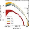 |
Fig. 1 Mean power spectra |
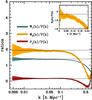 |
Fig. 2 Ratio between the spectra |

Along with the measurements in real space, we also measured two-point statistics in redshift space by means of the distant-observer approximation, i.e., shifting the position of dark matter halos along the x-axis x → x + vx/H0 where vx is the x-component of the peculiar velocity of the halo center of mass. We keep Fourier modes up to a ~60% of the Nyquist frequency kNy = 0.89 h Mpc-1, where the corrections due to the assignment scheme are accurate (e.g., Cole et al. 2005).
Different power spectra defined in the text.
In Fig. 1 we show the mean of the real-space power
spectra  and
and  (computed using the full luminosity range) with the corresponding standard deviation
obtained from the ensemble of realizations of the L-BASICC simulation. At first glance,
the estimates of marked power spectra
behave as scaled versions of .
Indeed, on large scales (k ≲ 0.04 h Mpc-1),
the ratios
(computed using the full luminosity range) with the corresponding standard deviation
obtained from the ensemble of realizations of the L-BASICC simulation. At first glance,
the estimates of marked power spectra
behave as scaled versions of .
Indeed, on large scales (k ≲ 0.04 h Mpc-1),
the ratios  are described well by a constant factor, as explicitly shown in Fig. 2. This suggests that the amplitude of the marked power
spectra
can be explained, as a first approximation, by including the information of the scaling
relation within a sort of luminosity bias. Indeed, the theoretical expectations
described in Appendix A and represented in Fig.
2 by the solid lines show that this is the case.
are described well by a constant factor, as explicitly shown in Fig. 2. This suggests that the amplitude of the marked power
spectra
can be explained, as a first approximation, by including the information of the scaling
relation within a sort of luminosity bias. Indeed, the theoretical expectations
described in Appendix A and represented in Fig.
2 by the solid lines show that this is the case.
A more careful analysis reveals, though, a scale dependence of the ratios
,
which is statistically significant even on large and intermediate scales k ≳ 0.04 h Mpc-1
(also present in redshift space). This is shown in the inset of Fig. 2. We note that
and
are equally affected by the nonlinear evolution of the underlying matter density field
and the exclusion effect (i.e., they are estimated from the same sample and thus the
smallest populated bin of separation is the same, albeit differently weighted), as well
as by the same scale-dependent halo-mass bias (see, e.g., Tinker et al. 2005). Therefore, the scale dependency observed in the
ratios
can be regarded as a signature of the distribution of the weights wiwj
within pairs at different separations, suggesting that the shape of the
luminosity-weighted power spectrum is sensitive to the scaling relation
 .
This is explored in Sect. 3.
.
This is explored in Sect. 3.
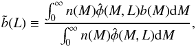
2.3.3. Introducing a new probe
As an attempt to isolate the signal of the clustering of the X-ray luminosity from the
unmarked power spectrum, we define  .
This fluctuation has zero mean,
.
This fluctuation has zero mean,  , and variance
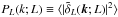 , where ⟨· ⟩ denotes an average over an ideal
ensemble of realizations. We refer to this variance as the luminosity power
spectrum. Thus defined, the variable δL accounts for the
fluctuations in the weighted number density with respect to the unweighted number
density. Since by construction both number densities share the same mean value, this
simple subtraction avoids us from having to assume that the observed mean number density
is the true mean density, and thus, the estimates of the luminosity power spectrum are
free of the so-called integral constraint (e.g., Peacock
& Nicholson 1991). Since the mean number density
, where ⟨· ⟩ denotes an average over an ideal
ensemble of realizations. We refer to this variance as the luminosity power
spectrum. Thus defined, the variable δL accounts for the
fluctuations in the weighted number density with respect to the unweighted number
density. Since by construction both number densities share the same mean value, this
simple subtraction avoids us from having to assume that the observed mean number density
is the true mean density, and thus, the estimates of the luminosity power spectrum are
free of the so-called integral constraint (e.g., Peacock
& Nicholson 1991). Since the mean number density
 only enters into the definition of δL as a
normalization, the possible difference between the observed and true number density
would equally affect all Fourier modes in PL(k;L)
by some constant factor. The estimates of the luminosity power spectrum are obtained
following the same procedure as described in the previous section, namely, a
shell-average of the estimate
only enters into the definition of δL as a
normalization, the possible difference between the observed and true number density
would equally affect all Fourier modes in PL(k;L)
by some constant factor. The estimates of the luminosity power spectrum are obtained
following the same procedure as described in the previous section, namely, a
shell-average of the estimate  with a shot-noise
correction SL:
with a shot-noise
correction SL: 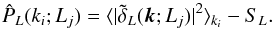 (6)According to the
definition of δL(r),
the luminosity power spectrum can be written as the combination of the
luminosity-weighted power spectra
(6)According to the
definition of δL(r),
the luminosity power spectrum can be written as the combination of the
luminosity-weighted power spectra 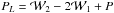 .
Thus, we can identify the shot-noise correction with
.
Thus, we can identify the shot-noise correction with
 , where
 .
Figure 1 shows the mean of the estimates of
PL(k)
as determined from the ensemble of N-body simulations (in the full luminosity
range), together with its standard deviation. As shown in Fig. 2, on large scales the shape of
.
Figure 1 shows the mean of the estimates of
PL(k)
as determined from the ensemble of N-body simulations (in the full luminosity
range), together with its standard deviation. As shown in Fig. 2, on large scales the shape of
 can be understood as a biased halo power spectrum, i.e., PL(k)/P(k) ~ const.,
which is even prevailing on intermediate scales (~0.1 h Mpc-1). In view of the
results shown in Appendix A, the luminosity power
spectrum can be thought of as directly probing the mean scaling relation.
can be understood as a biased halo power spectrum, i.e., PL(k)/P(k) ~ const.,
which is even prevailing on intermediate scales (~0.1 h Mpc-1). In view of the
results shown in Appendix A, the luminosity power
spectrum can be thought of as directly probing the mean scaling relation.
Table 1 summarizes the definitions of the different power spectra introduced in this section.
2.4. Two-point statistics as probe for cluster scaling relations
Generally, the information related to the parameters of a model explaining the observed two-point statistics can be extracted in three different ways: i) using the amplitude of the clustering signal; ii) using its full shape (e.g., Sánchez et al. 2012); or iii) isolating particular features such as the position of the baryonic acoustic peak in the correlation function (e.g., Anderson et al. 2012; Hong et al. 2012) or the turn-over in the power spectrum (e.g., Reid et al. 2010; Poole et al. 2013). We study the information content in cases i) and ii), and leave the assessment of the dependence of particular features for future studies, e.g., the acoustic peak in the correlation function, on the cluster scaling relations.
2.4.1. Amplitude
The information contained in the amplitude of the clustering signal can be extracted by
defining ratios of spectra by the underlying matter power spectrum or in a less
model-dependent fashion, by the clustering of the same population of objects at a given
luminosity (e.g., Norberg et al. 2002). As
suggested by panel b of Fig. 1, such ratios are
approximately constant on large scales (e.g., k ≲ 0.04 h Mpc-1).
We define for each realization q = 1, ··· ,N,
the following ratios: 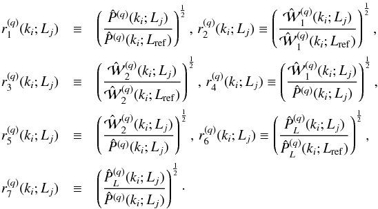 (7)Our
set of large-scale luminosity-dependent observables is then defined as
(7)Our
set of large-scale luminosity-dependent observables is then defined as
 , where
⟨·⟩δk denotes the average over
wavenumbers in the range δk = [0.01, 0.04] h Mpc-1.
The first three probes r1, 2, 3(L)
are defined as ratios of a given power spectrum in different luminosity bins with
respect to the same statistics, the latter measured in a fixed (reference) luminosity
bin Lref, thereby providing estimates of
relative biases of the marked spectra. The ratios r4, 5(L)
are instead defined by the unmarked power spectrum in the same luminosity bin, and we
refer to these as estimates of absolute bias4. Similarly, the ratios r6, 7(L)
are estimates of relative and absolute bias extracted from the luminosity power
spectrum. In these expressions Lref is taken as containing the value
L⋆ = 0.63 × 1044 erg s-1h-2,
the typical X-ray luminosity of galaxy clusters up to redshift z ~ 0.2 (Balaguera-Antolínez et al. 2012). We checked that our
results do not change substantially when other values of Lref are used,
except for the high-luminosity bins, wherein the clustering estimates display a low
signal-to-noise ratio. In Appendix A we show the
theoretical predictions for these ratios.
, where
⟨·⟩δk denotes the average over
wavenumbers in the range δk = [0.01, 0.04] h Mpc-1.
The first three probes r1, 2, 3(L)
are defined as ratios of a given power spectrum in different luminosity bins with
respect to the same statistics, the latter measured in a fixed (reference) luminosity
bin Lref, thereby providing estimates of
relative biases of the marked spectra. The ratios r4, 5(L)
are instead defined by the unmarked power spectrum in the same luminosity bin, and we
refer to these as estimates of absolute bias4. Similarly, the ratios r6, 7(L)
are estimates of relative and absolute bias extracted from the luminosity power
spectrum. In these expressions Lref is taken as containing the value
L⋆ = 0.63 × 1044 erg s-1h-2,
the typical X-ray luminosity of galaxy clusters up to redshift z ~ 0.2 (Balaguera-Antolínez et al. 2012). We checked that our
results do not change substantially when other values of Lref are used,
except for the high-luminosity bins, wherein the clustering estimates display a low
signal-to-noise ratio. In Appendix A we show the
theoretical predictions for these ratios.
2.4.2. Full shape
The measurements of the luminosity-weighted power spectrum shown in Sect. 2.3 revealed that the scaling relation
not only affects the amplitude of the weighted power spectra
 ,
but can also play a role in shaping their broad-band signal. To quantify the information
encoded in the full shape of the measured spectra P(k),
,
and PL(k),
we use their estimates in the range of wave numbers 0.02 ≤ k/(h Mpc-1) ≤ 0.2,
with
,
but can also play a role in shaping their broad-band signal. To quantify the information
encoded in the full shape of the measured spectra P(k),
,
and PL(k),
we use their estimates in the range of wave numbers 0.02 ≤ k/(h Mpc-1) ≤ 0.2,
with  Fourier modes, and use the
full X-ray luminosity range.
Fourier modes, and use the
full X-ray luminosity range.
As pointed out in Sect. 2.3, the variance of the fluctuations of the luminosity-weighted and luminosity power spectrum has a contribution that embodies two forms of randomness: one associated to the finite number of halos, the other to the distribution of the marks compared to its mean. These two effects are represented by Eq. (6). The shot-noise subtraction in the power spectrum of galaxy clusters is a delicate issue. As rare objects, clusters display number densities that are low enough to generate a shot-noise contribution that can be traceable even on the largest scales. As an example of its relevance, it can be seen that estimates of power spectra without shot-noise correction can generate a scale-dependent bias on scales where the ratios between corrected spectra were fairly described by a constant factor (see, e.g., Pollack et al. 2012). Strictly speaking, not subtracting the shot-noise correction from the estimates of power spectra is not an off base procedure, given that this correction is a model in itself and as such can be included in the modeling of the clustering signal. To asses the impact of the shot-noise correction in the amount of information we can retrieve, we consider below the case when the information content from the luminosity power spectrum is extracted from its shot-noise uncorrected estimate.
3. Results: information content
In this section we carry out a Fisher matrix analysis (see, e.g., Tegmark et al. 1997) in order to quantify the amount of information on
the mass-X ray luminosity scaling relation that our clustering-related observables contain.
Before proceeding, we recall that in the context of galaxy cluster experiments, one-point
statistics – such as cluster number counts – represent the standard probe for cosmological
parameters and scaling relations (e.g., Majumdar &
Mohr 2004; Lima & Hu 2004; Cunha & Evrard 2010; Pillepich et al. 2012). To compare our results – which are based on
two-point statistics – with a one-point statistics probe, we use the X-ray luminosity
function  (XLF hereafter) measured in
  equally log-spaced bins. Given
that the cosmological parameters are kept fixed throughout the analysis5, the information content in the XLF can provide a fair level of
comparison to assess the capability of the clustering probes in retrieving information on
the cluster scaling relation against the standard procedures. Our set of observables is
summarized as
equally log-spaced bins. Given
that the cosmological parameters are kept fixed throughout the analysis5, the information content in the XLF can provide a fair level of
comparison to assess the capability of the clustering probes in retrieving information on
the cluster scaling relation against the standard procedures. Our set of observables is
summarized as  (8)where the index
j runs from
(1, ··· , nℓ)
for the ratios rν(L),
(8)where the index
j runs from
(1, ··· , nℓ)
for the ratios rν(L),
 for the
power spectra, and
for the
power spectra, and  for the
XLF. For each observable, its mean
for the
XLF. For each observable, its mean  and covariance matrix C are given by
  and
and 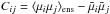 respectively, where ⟨·⟩ens denotes averages over the ensemble of realizations
of the L-BASICC simulations.
respectively, where ⟨·⟩ens denotes averages over the ensemble of realizations
of the L-BASICC simulations.
The Fisher matrix represents the ensemble average of the Hessian of the natural logarithm
of the likelihood function of a data set given a model, and its customary application aims
to forecast uncertainties of a set of model parameters from a given experiment. Our approach
is slightly different, though, since we aim to quantify the sensitivity of each of the
observables defined in Eq. (8) to the set of
parameters  (defined in Sect 2.2) using measurements and covariance
matrices directly extracted from the simulations. In other words, we assume perfect
knowledge of model and the covariance for our observables. Under the assumption that the
observables are drawn from a Gaussian distribution, the elements of the Fisher matrix
F are written as
(defined in Sect 2.2) using measurements and covariance
matrices directly extracted from the simulations. In other words, we assume perfect
knowledge of model and the covariance for our observables. Under the assumption that the
observables are drawn from a Gaussian distribution, the elements of the Fisher matrix
F are written as ![Mathematical equation: \begin{equation} \label{fis} F_{x y}=\frac{1}{2}{\rm Tr}\left[\textbf{C}^{-1}\textbf{C}_{,x}\textbf{C}^{-1}\textbf{C}_{,y}+\textbf{C}^{-1}\lp \bar{\bm{\mu}}_{,x}\bar{\bm{\mu}}_{,y}^{T}+\bar{\bm{\mu}}_{,y}\bar{\bm{\mu}}_{,x}^{T} \rp \right]|_{x=x_{\rm fid}}^{y=y_{\rm fid}}, \end{equation}](/articles/aa/full_html/2014/03/aa22029-13/aa22029-13-eq145.png) (9)where
,x ≡ ∂/∂x
and xfid denotes the fiducial values of the
parameters ,
defined in Sect. 2.2. The covariance matrix of the
parameters of the model is
(9)where
,x ≡ ∂/∂x
and xfid denotes the fiducial values of the
parameters ,
defined in Sect. 2.2. The covariance matrix of the
parameters of the model is  ,
and the marginal error of each parameter is obtained from the Cramér-Rao inequality
,
and the marginal error of each parameter is obtained from the Cramér-Rao inequality
 . We used
a double-side variation to accurately estimate the derivatives with respect to the
parameters. This leads us to computing 27(models) × 50(realizations) × 2(real and redshift-space estimates)× 3(marked spectra)× 10 (luminosity bins) = 8.1 × 10⁵ estimates of power
spectrum.
. We used
a double-side variation to accurately estimate the derivatives with respect to the
parameters. This leads us to computing 27(models) × 50(realizations) × 2(real and redshift-space estimates)× 3(marked spectra)× 10 (luminosity bins) = 8.1 × 10⁵ estimates of power
spectrum.
Three key aspects of our Fisher matrix analysis are taken into account. Firstly, by means
of the so-called D’Agostino K2 goodness-of-fit test, we have verified that the distribution
of the observables defined in Eq. (8) within
the suite of realizations of the N-body simulations is compatible to 95 per cent confidence with a normal
distribution within the ranges of the X-ray luminosity and wavenumbers of interest.
Secondly, we note that when computing the Fisher matrix for all our observables (with mean
values  ),
we omit the term containing the derivatives of the covariance matrix, since it adds spurious
information that shrinks the marginalized errors considerably (Carron 2013). Finally, when exploring the information content encoded
solely in the shape of the power spectra, we treat the amplitude of the mean spectra as a
nuisance parameter. Under the assumption that these amplitudes have flat or
Gaussian-distributed priors, analytical marginalization of the covariance matrix over these
parameters is possible (e.g., Lewis & Bridle
2002; Taylor & Kitching 2010). For a
flat prior on these amplitudes, the inverse of the marginalized covariance matrix is
obtained by subtracting the factor
),
we omit the term containing the derivatives of the covariance matrix, since it adds spurious
information that shrinks the marginalized errors considerably (Carron 2013). Finally, when exploring the information content encoded
solely in the shape of the power spectra, we treat the amplitude of the mean spectra as a
nuisance parameter. Under the assumption that these amplitudes have flat or
Gaussian-distributed priors, analytical marginalization of the covariance matrix over these
parameters is possible (e.g., Lewis & Bridle
2002; Taylor & Kitching 2010). For a
flat prior on these amplitudes, the inverse of the marginalized covariance matrix is
obtained by subtracting the factor ![Mathematical equation: \hbox{$\lp \textbf{C}^{-1}\bar{\bm{\mu}}^{T}\bar{\bm{\mu}}\rp/\lp{\rm Tr}[\bar{\bm{\mu}}\textbf{C}\bar{\bm{\mu}}^{T}]\rp$}](/articles/aa/full_html/2014/03/aa22029-13/aa22029-13-eq158.png) from the original inverted covariance matrix.
from the original inverted covariance matrix.
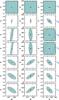 |
Fig. 3 Joint 1σ
error ellipses for the parameters { α,γ,σ } of the scaling relation
|
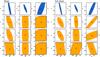 |
Fig. 4 Joint 1σ
error ellipses for the parameters { α,γ,σ } of the scaling relation
|
We quantify the information obtained from each of our observables by a figure of merit (FoM hereafter) defined as the inverse of the area of the marginalized 68% error ellipse of each pair of parameters. We also compute the total FoM given by the volume of the three-dimensional 68% error ellipsoid. We present the results from the Fisher matrix analysis in Figs. 3 and 4. Figure 6 condenses the FoM derived from our set of observables. We draw our conclusions based on these three figures.
3.1. Information content in the amplitude
Figure 3 shows the joint 1σ error ellipses obtained from the Fisher-matrix analysis of the set rν = 1, ··· , 7(L). The results are presented in real and redshift space. We next draw some conclusions based on this figure, in conjunction with Fig. 6.
-
The sensitivity to the parameters of the scaling relation varies little between the observables r1, 2, 3(L). This is also true when these observables are measured in redshift space. The estimates associated to absolute biases r4, 5(L) are slightly more sensitive to the signal of the spectra in redshift space.
-
When the ratios are defined by the unmarked power spectrum (i.e., r4, 5(L)), the marginalized errors on the amplitude, σα, decrease while σγ increases, with a net decrease in the total FoM. Therefore, the set r1, 2, 3(L) proves to be more sensitive to the set {γ,σ}, while the set r4, 5(L) sets tighter constraints on amplitude α.
-
The estimates of relative bias extracted from the luminosity power spectrum r6(L) generate FoM that are approximately two orders of magnitude above those obtained from the luminosity weighted power spectrum, say r3(L), marking a noticeable improvement. The total FoM of derived from this probe is only ~40 times below the one derived from the XLF. On the other hand, the estimate of absolute bias r7(L) sets poor constraints.
-
In general, better constraints are obtained from the estimates of relative bias. As pointed out before, the selection of the reference luminosity does not affect our conclusions, except for very high values of Lref.
We conclude that, regarding the amplitude of the cluster power spectrum, the unmarked analysis is accurate enough and no extra-information is gained by measuring the luminosity dependence of the amplitude of the luminosity-weighted power spectrum. On the other hand, we have shown that the estimates of luminosity bias obtained from the luminosity power spectrum, r6(L), allows us to retrieve an amount of information on the scaling relation that is only one order of magnitude below the one characterizing the XLF.
3.2. Information content in the full shape
Figure 4 shows the error ellipses from the analysis
of the full shape of the power spectra ,
,
and  , both
in real and in redshift space, with Fourier modes in the range 0.02 < k/(h Mpc-1) < 0.2.
The left hand panel in that figure corresponds to the results obtained after marginalizing
the covariance matrix of each observable with respect to an overall amplitude, while the
right hand panel shows results obtained after using the information encoded in the full
shape. This figure confirms the intuitive prediction that more information (smaller error
ellipses) is gained when the full shape is used in the analysis. We complement the
information shown in Fig. 4 with the information
shown in Figs. 5 and 6. From these we conclude the following.
, both
in real and in redshift space, with Fourier modes in the range 0.02 < k/(h Mpc-1) < 0.2.
The left hand panel in that figure corresponds to the results obtained after marginalizing
the covariance matrix of each observable with respect to an overall amplitude, while the
right hand panel shows results obtained after using the information encoded in the full
shape. This figure confirms the intuitive prediction that more information (smaller error
ellipses) is gained when the full shape is used in the analysis. We complement the
information shown in Fig. 4 with the information
shown in Figs. 5 and 6. From these we conclude the following.
-
The marked power spectra
generate higher FoM compared to P(k), due mainly to their
sensitivity to the slope of the scaling relation γ. These three
spectra are almost equally sensitive to the intrinsic scatter σ and the amplitude
α.
-
A gain in information content on the scaling relation is obtained from the luminosity power spectrum, with FoM increased approximately by an order of magnitude over what is obtained with
 ,
or, ~40 times below what
characterizes the information encoded in the XLF.
,
or, ~40 times below what
characterizes the information encoded in the XLF. 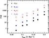
Fig. 5 FoM obtained from the 1σ error ellipsoids of the parameters of the scaling relation as a function of the maximum wavenumber kmax. The FoM shown correspond to the information contained in the full shape of the clustering probes.
-
Figure 5 shows the behavior of the FoM related to the full shape of the observables
,
,
and ,
as a function of the maximum wavenumber used in the analysis, kmax. We
see that the ratio of the FoM contained in the luminosity power spectrum
PL(k)
to that of the unweighted power spectrum P(k) ranges from a factor
102 with
kmax ~ 0.07 h Mpc-1
to ~20 with
kmax ~ 0.2 h Mpc-1.
The trend of the different FoM with the maximum wavenumber is as expected; i.e, the
higher the number of Fourier modes, the higher the content of information in the
Fisher matrix. -
To emphasize the relevance of the shot-noise correction, we repeated our analysis using the shot-noise uncorrected estimates of the different power spectra. As a result, the FoM obtained are higher than those presented in Fig. 6, as has been explicitly portrayed for the case of the shot-noise uncorrected luminosity power spectrum (denoted by
 ). The ratios between the
FoM obtained from the uncorrected estimates to those derived from the corrected ones
(using their full shape as probes) are ~3, 21, and 23 for
). The ratios between the
FoM obtained from the uncorrected estimates to those derived from the corrected ones
(using their full shape as probes) are ~3, 21, and 23 for  ,
and PL
respectively, illustrating how sensitive the clustering signal of galaxy clusters to
the shot-noise correction is. Furthermore, the total FoM associated to
is a factor ~2.5 smaller than the corresponding
value obtained from the XLF, which is noticeable if we compare it to the factors
~15 and
~2 × 10³ derived from
,
and PL
respectively, illustrating how sensitive the clustering signal of galaxy clusters to
the shot-noise correction is. Furthermore, the total FoM associated to
is a factor ~2.5 smaller than the corresponding
value obtained from the XLF, which is noticeable if we compare it to the factors
~15 and
~2 × 10³ derived from
 and P(k) respectively6. The shot-noise correction (either Poisson-like
or scale-dependent) is always demanded, if not in the measurement, then in the model
adopted for interpreting the clustering signal. Not doing that can lead to biased
interpretations of the observed power spectra, which degenerate into spurious tight
constraints on the parameters of interest.
and P(k) respectively6. The shot-noise correction (either Poisson-like
or scale-dependent) is always demanded, if not in the measurement, then in the model
adopted for interpreting the clustering signal. Not doing that can lead to biased
interpretations of the observed power spectra, which degenerate into spurious tight
constraints on the parameters of interest.
In summary, Fig. 6 attempts to answer the question posed by the title of this paper. The improvement in the FoM obtained from the luminosity power spectrum with respect to the standard probes (i.e., unweighted clustering analysis) represents the main result of our analysis.
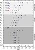 |
Fig. 6 FoMs obtained from the 1σ error ellipses of each pair of parameters
of the scaling relation, taken from the different observables μj defined in Eq.
(8). By FoM we denote the figure of
merit computed as the volume of the 3-dimensional 68% error ellipsoid. To facilitate the
understanding of this figure, the dark gray, gray and light gray areas denote
observables accounting for the amplitude, the shape and the full shape of power
spectra respectively. Results are shown in real space. Noticeably, the luminosity
power spectrum PL provides
more information regarding the scaling relation than the luminosity-weighted
spectra, and display a total FoM that is ~102 times that of the unweighted power spectrum. We
show the estimates derived from the luminosity power spectrum
|
4. Discussion and conclusions
In this paper we aimed to explore the capability of the so-called marked statistics of
galaxy clusters to retrieve information on the links between cluster masses and cluster
X-ray luminosities. To this end, we assigned X-ray luminosities to dark matter halos in a
suite of N-body
simulations and measured luminosity-weighted power spectra
and luminosity power spectrum ,
as defined in Sect. 2.3. The luminosity power spectrum
has been defined such that it directly measures the clustering of X-ray luminosity. The
definition of the luminosity power spectrum can be extrapolated to other probes of two-point
statistics, such as the angular power spectrum. This can be especially suitable in cases
where no redshift-information is available and clusters are identified by a redshift
independent intrinsic property, such as the SZ signal (e.g., Planck Collaboration XXIX. 2014).
We extracted the information related to the scaling relation by dissecting the clustering
signal in three different parts: first, we isolated the large-scale information on the power
spectra measured in different luminosity bins, and measured estimates of luminosity bias.
Second, we explored the information encoded in the shape of the clustering signal, and
third, we considered their full shape (i.e., shape and amplitude). This yields a total of
twelve observables. By carrying out a Fisher matrix analysis, we quantified the amount of
information regarding the cluster scaling relation from each of these observables through
the definition of a FoM. In terms of the amplitude, we showed that the
information encoded in the estimates of cluster luminosity bias measured from the unweighted
power spectrum P(k) is close to what is obtained
from the bias of the weighted spectra  ,
so that no sensitive gain of information is achieved. However, a relevant increase in the
information content is obtained when estimates of relative bias are extracted from the
luminosity power spectrum, reaching FoM that are only one order of magnitude below the
values derived from the XLF analysis. Similarly, when exploring the information content
within the full shape of the power spectra, we found that the information associated to
PL(k)
overcomes that of the spectra
and P(k): the resulting FoM of the
PL is a factor of
~100 (~10) with respect to that of the unweighted
(weighted) power spectrum. The gain in information obtained from the estimates of
the luminosity power spectrum with respect to the unweighted analysis represents
the main result of this paper.
,
so that no sensitive gain of information is achieved. However, a relevant increase in the
information content is obtained when estimates of relative bias are extracted from the
luminosity power spectrum, reaching FoM that are only one order of magnitude below the
values derived from the XLF analysis. Similarly, when exploring the information content
within the full shape of the power spectra, we found that the information associated to
PL(k)
overcomes that of the spectra
and P(k): the resulting FoM of the
PL is a factor of
~100 (~10) with respect to that of the unweighted
(weighted) power spectrum. The gain in information obtained from the estimates of
the luminosity power spectrum with respect to the unweighted analysis represents
the main result of this paper.
The results presented show, though, that the XLF still encodes more astrophysical information than our best clustering probe, the luminosity power spectrum. This implies that the contribution of the latter in the constraints of astrophysical parameters within a joint XLF-clustering analysis could be subdominant, at least in the case where the cosmological sector is fixed. In a more realistic scenario, though, Pillepich et al. (2012) show that the combination of cluster number counts and the standard (i.e, unweighted) angular cluster power spectrum for the eROSITA experiment can set constraints that are tighter than those derived from the number counts alone. Nevertheless, these authors emphasize that this trend can be reversed after variations in the selection function of the sample in their study. A direct comparison between our approach and the Pillepich et al. (2012) analysis is not applicable, since, as we already pointed out, we are not interested in assessing the ability of a certain model to explain a given experiment, and also because we have kept the cosmological parameters fixed, thereby ignoring all possible correlations between the cosmological and the astrophysical sector. In view of our results, it can be expected that the joint analysis of number counts and some X-property angular power spectrum can contribute to improving the FoM in the work of Pillepich et al. (2012). This is currently under study.
An obvious question arises, as to the feasibility of the clustering signal to set precise constraints on cluster scaling relations in future galaxy-cluster surveys. From the observational point of view, the volume of the N-body simulations we used to create cluster catalogs mimics that of a full-sky complete sample to a maximum redshift of z ~ 0.3. The resulting mean number density resembles what is expected from the eROSITA experiment (Pillepich et al. 2012). Therefore the precision to which only the scaling relation could be constrained from these forthcoming samples – when redshifts are available and using PL(k) – can be of the same order as that obtained from our analysis. On the other hand, the volumes that will be probed by the forthcoming surveys will generate statistical errors on the estimates of power spectra that might be compatible to the systematic errors present when modeling clustering. This situation is especially noticeable on small scales – probed by a large number of modes – where the clustering signal is dominated by the nonlinear evolution of the matter density field, the scale-dependent halo-mass bias, the halo exclusion, and ultimately baryonic effects.
In Fig. 6 we displayed our results such that relevant FoM are obtained, especially for the luminosity power spectrum, when we include Fourier modes up to a scale of k ~ 0.2 h Mpc-1 in our analysis. From a theoretical perspective, extending the analysis to such values of wavenumbers might be a point of concern. On these scales, highly complex processes (e.g., nonlinear evolution of the matter density field, scale-dependent halo biasing and halo exclusion effect) become non-negligible. In the past two decades, major progress in the understanding of some of these processes has been accomplished. In that regard, there are several attempts to describe the nonlinear evolution of dark matter, either based on numerical fits to N-body simulations (e.g., Peacock & Dodds 1996; Smith et al. 2003) or on theoretical predictions (e.g., Bernardeau et al. 2002; Crocce & Scoccimarro 2006; McDonald 2007; Matsubara 2011). The link between dark matter and halos – the halo-mass bias – has also been an active area of research, regarding its nature and fitting formulae for its implementation. Even if these theoretical predictions accurately describe the results from N-body simulations, baryonic effects within galaxy clusters (e.g., radiative cooling, star formation, feedback mechanism due to AGN and supernova) can severely spoil the expectations of modeling the observed clustering signal to the accuracy achieved by state-of-the art cosmological simulations of dark matter. Indeed, such effects have been shown to substantially modify the abundance and clustering of clusters with respect to pure dark matter-based predictions (e.g., Stanek et al. 2009; Rudd et al. 2008; van Daalen et al. 2011; Cui et al. 2012; Balaguera-Antolínez & Porciani 2013). In view of the plethora of models accounting for the baryonic effects that shape the intracluster medium and the small scales (astrophysical, instead of cosmological) where these effects take place, precise modeling of the abundance and clustering of galaxy clusters based on N-body simulations is still far from being achieved. Even though it is beyond the scope of this paper to discuss the impact of the systematic effects present on the modeling of the quantities mentioned above, we recognize their relevance in extracting accurate information regarding the parameters describing the observed clustering pattern of galaxy clusters (especially using the luminosity power spectrum) from forthcoming galaxy and galaxy cluster surveys such as eROSITA, DES (The Dark Energy Survey Collaboration 2005), or Euclid (Laureijs et al. 2011). We notice that the only model that we have explicitly implemented in our analysis makes the assumption that the halo distribution behaves like a Poisson point process, which is a debatable hypothesis (see, e.g., Casas-Miranda et al. 2002; Smith et al. 2007). With this assumption, the shot-noise correction of the halo power spectrum is represented by subtracting a white noise from the raw power spectrum. However, even simple toy models assuming spherical halos reveal a scale-dependent shot noise. We discuss this briefly in Appendix B.
The weighted two-point statistics proves itself to be an interesting tool for characterizing the explicit dependence of the clustering of galaxy clusters on intrinsic properties. The implementation of these statistics, either in Fourier space (as we have shown in this paper) or in configuration space (see, e.g., Sheth 2005), can contribute setting tight constraints on the parameters that characterize the physics of the intra-cluster medium, interestingly intertwining cosmology and astrophysics on the galaxy cluster-scale.
Online material
Appendix A: The cluster-mass bias
The ratios rν(L)
defined in Sect. 2.4.1 can be predicted under the
assumption that, on large scales, dark matter halos of a given mass M are biased tracers of
the underlying dark matter distribution. In the so-called local bias model, to zeroth
order in perturbation theory (e.g., Cooray &
Sheth 2002), this is expressed as P(k;M) = b2(M)Pmat(k),
where Pmat(k) denotes the
power spectrum of the dark matter and b(M) is a scale-independent
halo-mass bias. Given a halo mass function n(M)dM (i.e.,
the number of dark matter halos with masses between M and M + dM
per unit comoving volume) and a selection function
 (i.e., the probability of having a cluster with mass M given some selection
criteria), the real-space marked power spectra can be written as
(i.e., the probability of having a cluster with mass M given some selection
criteria), the real-space marked power spectra can be written as
 (e.g., Cooray & Sheth 2002; Sheth 2005), where
 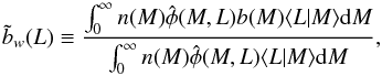 (A.1)and
 (A.2)is the
effective cluster-matter bias. For a given bin of X-ray luminosity, the selection
function φ(M,L) can be expressed as the
average of the scaling relation
given by Eq. (1) in that luminosity bin.
The ratios r1, 2, 3(L)
in real space can therefore be interpreted as estimates of b(L)/b(Lref),
bw(L)b(L) /(b(Lref)bw(Lref)),
and bw(L)/bw(Lref)
respectively. Also, the information contained in the ratio r4(L) is the same as
contained in the ratio r5(L), since these
are estimates of the ratio (bw(L) /b(L))1/2
and bw(L)/b(L)
respectively. Accordingly, the luminosity power spectrum can be written as
(A.2)is the
effective cluster-matter bias. For a given bin of X-ray luminosity, the selection
function φ(M,L) can be expressed as the
average of the scaling relation
given by Eq. (1) in that luminosity bin.
The ratios r1, 2, 3(L)
in real space can therefore be interpreted as estimates of b(L)/b(Lref),
bw(L)b(L) /(b(Lref)bw(Lref)),
and bw(L)/bw(Lref)
respectively. Also, the information contained in the ratio r4(L) is the same as
contained in the ratio r5(L), since these
are estimates of the ratio (bw(L) /b(L))1/2
and bw(L)/b(L)
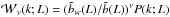
respectively. Accordingly, the luminosity power spectrum can be written as  (A.3)from which the
predictions for the ratios r6, 7(L)
can be readily obtained. According to Eq. (1), the moments of the luminosity L are linked to the scaling relation via
(A.3)from which the
predictions for the ratios r6, 7(L)
can be readily obtained. According to Eq. (1), the moments of the luminosity L are linked to the scaling relation via
 .
Therefore, the bias
.
Therefore, the bias  is directly sensitive to the mean of the scaling relation, yet indirectly (only through
)
to the intrinsic scatter.
is directly sensitive to the mean of the scaling relation, yet indirectly (only through
)
to the intrinsic scatter.
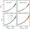 |
Fig. A.1 Ratio r3(L) (top panels) defined in Eq. (7), and luminosity bias b(L) (bottom panels) obtained in the range 0.02 ≤ k/(h Mpc-1) ≤ 0.08. Results are shown in real (right panel) and redshift (left panel) space. For readability, we only show the standard deviation obtained from the N-body simulations with shaded regions. The lines represent the predictions presented in Sect. 2.4.1 using expressions for the halo-mass bias as reported by different authors, MW: Mo & White (1996); ST: Sheth & Tormen (1999); T: Tinker et al. (2010); and P: Pillepich et al. (2010). |
The redshift-space estimates of the ratios rν(L)
can be obtained in a similar way. Under the plane-parallel approximation, the
large-scale signal of the redshift-space cluster power spectrum Ps(k;L)
can be described by the so-called Kaiser effect (e.g., Kaiser 1987; Hamilton 1998)
Ps(k;L) = (1 + 2β/3 + β2/5)P(k;L), where
 and
f ≡ dlnD(a)/dlna
is the growth index (D(a) represents the growth
factor) (e.g., Peebles 1980). Given the cosmology
and redshift output of the L-BASICC simulations that we used, f = 0.44. The Kaiser
effect can be generalized to the marked power spectra (e.g., Skibba et al. 2006) as
and
f ≡ dlnD(a)/dlna
is the growth index (D(a) represents the growth
factor) (e.g., Peebles 1980). Given the cosmology
and redshift output of the L-BASICC simulations that we used, f = 0.44. The Kaiser
effect can be generalized to the marked power spectra (e.g., Skibba et al. 2006) as 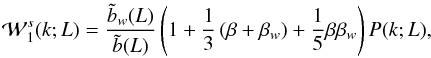 (A.4)and
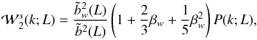 (A.5)where
 . We
have checked whether these expressions describe the ratios rν(L).
To this end, the halo abundance n(M) is taken to be described by
the fitting formulae of Jenkins et al. (2001),
which is suitable for simulations such as the L-BASICC. A crucial step is to choose the
halo-mass bias b(M). In Fig. A.1 we show predictions for the ratio r3(L), obtained using
some examples of prescriptions for this quantity: Mo
& White (1996), Sheth & Tormen
(1999), Tinker et al. (2010). and Pillepich et al. (2010). To witness the performance
of these prescriptions, the bottom panels in Fig. A.1 show the luminosity bias obtained similar to what is described by Eq.
(7), using the estimates of the matter
power spectrum of the L-BASICC II simulation. This figure shows that i) as established
by a number of studies, a scale-independent halo-mass bias is a fair modeling of the
cluster power spectrum on large scales; ii) the Kaiser effect is a good description of
the redshift-space power spectra, at least within the range of masses and scales probed
by our analysis (see, e.g., Bianchi et al. 2012,
for a broader discussion on this subject); iii) when assessing the ability of a model to
retrieve either cosmological or astrophysical information from one or two-point
statistics, extreme caution is required in view of the discrepancies observed between
models and the simulations. In particular, more accurate models of halo-mass function
and halo-mass bias are demanded, given the small statistical errors expected from
forthcoming surveys (see, e.g., Cunha & Evrard
2010; Wu et al. 2010; Smith et al. 2012) with volumes comparable to that of
the L-BASICC simulation. The differences between the different fitting formulae
presented in Fig. A.1 can be caused by several
effects, namely, the difference cosmological models and/or parameters used in the
N-body
simulations used to fit each of them, the characteristics of the halo-identification
algorithm (which introduces systematic effects both in the mass function and the
halo-mass bias), and the way the biases are measured (i.e, either from the correlation
function, the power spectrum, or by means of count-in cells experiments). It is beyond
the scope of this work to analyze these differences in detail; however, we note that
different fitting formulae can provide a good description of the measured luminosity
bias at different ranges of X-ray luminosity. In particular, the results from Tinker et al. (2010) generate a fair description for
luminosities above ~3 × 1043 h-2 erg s-1.
Lower luminosities correspond to halos defined by a relatively low number of dark matter
particles, where resolution effects can be relevant. Finally, iv) the discrepancies
between the different prescription of halo-mass bias are slightly diminished when we
work with estimates of relative biases instead of absolute biases.
. We
have checked whether these expressions describe the ratios rν(L).
To this end, the halo abundance n(M) is taken to be described by
the fitting formulae of Jenkins et al. (2001),
which is suitable for simulations such as the L-BASICC. A crucial step is to choose the
halo-mass bias b(M). In Fig. A.1 we show predictions for the ratio r3(L), obtained using
some examples of prescriptions for this quantity: Mo
& White (1996), Sheth & Tormen
(1999), Tinker et al. (2010). and Pillepich et al. (2010). To witness the performance
of these prescriptions, the bottom panels in Fig. A.1 show the luminosity bias obtained similar to what is described by Eq.
(7), using the estimates of the matter
power spectrum of the L-BASICC II simulation. This figure shows that i) as established
by a number of studies, a scale-independent halo-mass bias is a fair modeling of the
cluster power spectrum on large scales; ii) the Kaiser effect is a good description of
the redshift-space power spectra, at least within the range of masses and scales probed
by our analysis (see, e.g., Bianchi et al. 2012,
for a broader discussion on this subject); iii) when assessing the ability of a model to
retrieve either cosmological or astrophysical information from one or two-point
statistics, extreme caution is required in view of the discrepancies observed between
models and the simulations. In particular, more accurate models of halo-mass function
and halo-mass bias are demanded, given the small statistical errors expected from
forthcoming surveys (see, e.g., Cunha & Evrard
2010; Wu et al. 2010; Smith et al. 2012) with volumes comparable to that of
the L-BASICC simulation. The differences between the different fitting formulae
presented in Fig. A.1 can be caused by several
effects, namely, the difference cosmological models and/or parameters used in the
N-body
simulations used to fit each of them, the characteristics of the halo-identification
algorithm (which introduces systematic effects both in the mass function and the
halo-mass bias), and the way the biases are measured (i.e, either from the correlation
function, the power spectrum, or by means of count-in cells experiments). It is beyond
the scope of this work to analyze these differences in detail; however, we note that
different fitting formulae can provide a good description of the measured luminosity
bias at different ranges of X-ray luminosity. In particular, the results from Tinker et al. (2010) generate a fair description for
luminosities above ~3 × 1043 h-2 erg s-1.
Lower luminosities correspond to halos defined by a relatively low number of dark matter
particles, where resolution effects can be relevant. Finally, iv) the discrepancies
between the different prescription of halo-mass bias are slightly diminished when we
work with estimates of relative biases instead of absolute biases.
Appendix B: Halo exclusion
Dark matter halos are not point-like objects. As a consequence, the idea that their
spatial distribution can be described as a Poisson-point process drawn from a
realization of an underlying continuous field with a positive correlation function
(Peebles 1980) is, strictly speaking, not a
realistic assumption. So far, a statistical description of halo distribution that takes
their finite size into account is not fully accomplished. Instead, simple geometrical
approaches have been developed to empirically model the exclusion effect within the
context of the two-point correlation function. Here we briefly illustrate how this model
works. Assuming that we can assign a radius to each spherical halo, the correlation
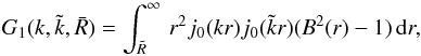
function can be written as (e.g., Porciani &
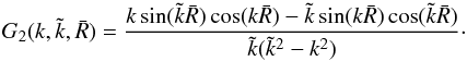
Giavalisco 2002) ![Mathematical equation: \appendix \setcounter{section}{2} \begin{equation} \label{ex-geo} \xi_{\rm h}(r;M,M')= \begin{cases} b(M)b(M')B^{2}(r)\xi_{\rm mat}(r) & r > \bar{R}(M,M'),\\[2mm] -1 & r\leq \bar{R}(M,M'), \end{cases} \end{equation}](/articles/aa/full_html/2014/03/aa22029-13/aa22029-13-eq226.png) (B.1)where
(B.1)where
 ,
with ⟨R|M ⟩ denoting the expected
radius of a cluster with mass M. In this expression, b(M)
denotes the dark-matter halo scale-independent bias, B(r)
denotes a possible scale-dependency in the halo-matter bias (e.g., Tinker et al. 2005), while ξmat(r) is the full
nonlinear matter correlation function. For halos with masses within an infinitesimally
narrow range, this expression predicts a sharp transition towards ξh(r) = −1 at a scale
equal to twice the radius of the halo. This transition becomes smoother when halos with
different masses (and thus sizes) are included. In Fourier space, the exclusion is
translated to a lack of power on small scales, which goes counter to the effect of the
nonlinear clustering. Since the exclusion effect is more evident when more massive halos
are considered, such lack of power displays a clear trend with the characteristic mass
(or X-ray luminosity) of the sample. The halo power spectrum from Eq. (B.1) can be separated into three components:
,
with ⟨R|M ⟩ denoting the expected
radius of a cluster with mass M. In this expression, b(M)
denotes the dark-matter halo scale-independent bias, B(r)
denotes a possible scale-dependency in the halo-matter bias (e.g., Tinker et al. 2005), while ξmat(r) is the full
nonlinear matter correlation function. For halos with masses within an infinitesimally
narrow range, this expression predicts a sharp transition towards ξh(r) = −1 at a scale
equal to twice the radius of the halo. This transition becomes smoother when halos with
different masses (and thus sizes) are included. In Fourier space, the exclusion is
translated to a lack of power on small scales, which goes counter to the effect of the
nonlinear clustering. Since the exclusion effect is more evident when more massive halos
are considered, such lack of power displays a clear trend with the characteristic mass
(or X-ray luminosity) of the sample. The halo power spectrum from Eq. (B.1) can be separated into three components:
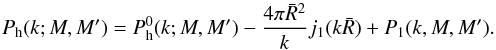 (B.2)The first term
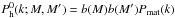 is the halo power
spectrum with a scale-independent bias. The second term is the Fourier transform of the
−1 in Eq. (B.1), where j1(x) denotes the
spherical Bessel function of first order. The third contribution can be written as
is the halo power
spectrum with a scale-independent bias. The second term is the Fourier transform of the
−1 in Eq. (B.1), where j1(x) denotes the
spherical Bessel function of first order. The third contribution can be written as
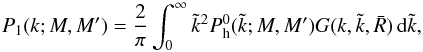 (B.3)
(B.3)
where the kernel  is
given by
is
given by  , with
 (B.4)and
 (B.5)In the limit
 (i.e., no halo exclusion), both the second term on the right hand side of Eq. (B.3) and the kernel G2 go to zero.
In that case a nonlinear contribution to the cluster power spectrum relies on the
behavior of the scale-dependent halo-mass bias B(r). In
the limit of an homogeneous distribution, we end up with a power spectrum of the form
(i.e., no halo exclusion), both the second term on the right hand side of Eq. (B.3) and the kernel G2 go to zero.
In that case a nonlinear contribution to the cluster power spectrum relies on the
behavior of the scale-dependent halo-mass bias B(r). In
the limit of an homogeneous distribution, we end up with a power spectrum of the form
 . Thus, to obtain an
unbiased estimation of the cluster power spectrum (of spherically symmetric
nonoverlapping clusters), this last term would need to be subtracted from the raw
estimates (as in Eq. (3)), together with
the white shot noise
. Thus, to obtain an
unbiased estimation of the cluster power spectrum (of spherically symmetric
nonoverlapping clusters), this last term would need to be subtracted from the raw
estimates (as in Eq. (3)), together with
the white shot noise  .
The combination of these two effects can be regarded as scale-dependent shot-noise.
.
The combination of these two effects can be regarded as scale-dependent shot-noise.
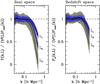 |
Fig. B.1 Halo exclusion: ratio between the measured cluster power spectrum described in Sect. 2.3 and the expected linear cluster power spectrum b2(L)Pmat(k), for clusters in four different bins of X-ray luminosity characterized by a luminosity Li, with L3 > L2 > L1. The luminosity bias b2(L) is that measured from the simulations. The shaded regions and the solid line represent the standard deviation and the mean, respectively, obtained from the N-body simulations. |
Figure B.1 depicts the halo exclusion effect as measured from the ensemble of halos presented in Sect. 2.1. As pointed out above, the strength of the effect scales with the luminosities (or masses) of the objects considered in the analysis. Therefore, this signal can be used to retrieve information on the underlying scaling relation (e.g., mass-X-ray luminosity when analyzing cluster samples or the mass-number of hosted galaxies when analyzing a galaxy redshift survey) (e.g., Porciani & Giavalisco 2002). Finally, the exclusion effect is attenuated when observed in redshift space, simply because pairs of halos are observed to be closer due to their peculiar velocities. For instance, exploring the power spectrum obtained from the full luminosity sample shows that in real space exclusion sets in at k ~ 0.2 h Mpc-1, while this value shifts to ~0.3 h Mpc-1 in redshift space.
The Hubble constant H0 being in units of 100 km s-1 Mpc-1.
If not explicitly written, X-ray luminosities and masses are expressed in units of 1044 h-2 erg s-1 h-2 and 1014 h-1 M⊙ respectively.
We denote by  the estimates of the quantity f.
We mean absolute with respect to the unmarked cluster power spectrum, not to the matter power spectrum.
Even though the dependence on cosmological parameters of the cluster number counts and luminosity function is slightly different, their dependence on the parameters of the scaling relation is the same.
The Fisher matrix of PLis not the sum of the Fisher matrix of the weighted spectra.
Acknowledgments
I am grateful to Raúl Angulo for making the L-BASICC II simulations available. I thank Cristiano Porciani and Nina Roth for useful discussions and suggestions, as well as the anonymous referee for comments that helped improve the presentation and content of the manuscript. I acknowledge support through the SFB-Transregio 33 “The Dark Universe” by the Deutsche Forschungsgemeinschaft (DFG).
References
- Allen, S. W., Evrard, A. E., & Mantz, A. B. 2011, ARA&A, 49, 409 [NASA ADS] [CrossRef] [Google Scholar]
- Anderson, L., Aubourg, E., Bailey, S., et al. 2012, MNRAS, 427, 3435 [Google Scholar]
- Angulo, R. E., Baugh, C. M., Frenk, C. S., & Lacey, C. G. 2008, MNRAS, 383, 755 [NASA ADS] [CrossRef] [Google Scholar]
- Balaguera-Antolínez, A., & Porciani, C. 2013, JCAP, 4, 22 [Google Scholar]
- Balaguera-Antolínez, A., Sánchez, A. G., Böhringer, H., et al. 2011, MNRAS, 413, 386 [NASA ADS] [CrossRef] [Google Scholar]
- Balaguera-Antolínez, A., Sánchez, A. G., Böhringer, H., & Collins, C. 2012, MNRAS, 425, 2244 [NASA ADS] [CrossRef] [Google Scholar]
- Bardeen, J. M., Bond, J. R., Kaiser, N., & Szalay, A. S. 1986, ApJ, 304, 15 [NASA ADS] [CrossRef] [Google Scholar]
- Bernardeau, F., Colombi, S., Gaztañaga, E., & Scoccimarro, R. 2002, Phys. Rep., 367, 1 [NASA ADS] [CrossRef] [EDP Sciences] [MathSciNet] [Google Scholar]
- Bianchi, D., Guzzo, L., Branchini, E., et al. 2012, MNRAS, 427, 2420 [NASA ADS] [CrossRef] [Google Scholar]
- Böhringer, H., Collins, C. A., Guzzo, L., et al. 2002, ApJ, 566, 93 [NASA ADS] [CrossRef] [Google Scholar]
- Carron, J. 2013, A&A, 551, A88 [NASA ADS] [CrossRef] [EDP Sciences] [Google Scholar]
- Casas-Miranda, R., Mo, H. J., Sheth, R. K., & Boerner, G. 2002, MNRAS, 333, 730 [NASA ADS] [CrossRef] [Google Scholar]
- Cole, S., Percival, W. J., Peacock, J. A., et al. 2005, MNRAS, 362, 505 [NASA ADS] [CrossRef] [Google Scholar]
- Cooray, A., & Sheth, R. 2002, Phys. Rep., 372, 1 [NASA ADS] [CrossRef] [Google Scholar]
- Crocce, M., & Scoccimarro, R. 2006, Phys. Rev. D, 73, 063519 [NASA ADS] [CrossRef] [Google Scholar]
- Cui, W., Borgani, S., Dolag, K., Murante, G., & Tornatore, L. 2012, MNRAS, 423, 2279 [NASA ADS] [CrossRef] [Google Scholar]
- Cunha, C. E., & Evrard, A. E. 2010, Phys. Rev. D, 81, 083509 [NASA ADS] [CrossRef] [Google Scholar]
- Finoguenov, A., Reiprich, T. H., & Böhringer, H. 2001, A&A, 368, 749 [NASA ADS] [CrossRef] [EDP Sciences] [Google Scholar]
- Frigo, M., & Johnson, S. G. 2012, Astrophysics Source Code Library ascl:1201.015 [Google Scholar]
- Giodini, S., Pierini, D., Finoguenov, A., et al. 2009, ApJ, 703, 982 [NASA ADS] [CrossRef] [Google Scholar]
- Hamilton, A. J. S. 1998, in The Evolving Universe, ed. D. Hamilton, Astrophys. Space Sci. Lib., 231, 185 [Google Scholar]
- Hockney, R. W., & Eastwood, J. W. 1988, Computer simulation using particles (Beistol: Hilger) [Google Scholar]
- Hong, T., Han, J. L., Wen, Z. L., Sun, L., & Zhan, H. 2012, ApJ, 749, 81 [NASA ADS] [CrossRef] [Google Scholar]
- Jenkins, A., Frenk, C. S., White, S. D. M., et al. 2001, MNRAS, 321, 372 [NASA ADS] [CrossRef] [MathSciNet] [Google Scholar]
- Kaiser, N. 1986, MNRAS, 222, 323 [NASA ADS] [CrossRef] [Google Scholar]
- Kaiser, N. 1987, MNRAS, 227, 1 [NASA ADS] [CrossRef] [Google Scholar]
- Kravtsov, A. V., & Borgani, S. 2012, ARA&A, 50, 353 [NASA ADS] [CrossRef] [Google Scholar]
- Laureijs, R., Amiaux, J., Arduini, S., et al. 2011 [arXiv:1110.3193] [Google Scholar]
- Lewis, A., & Bridle, S. 2002, Phys. Rev. D, 66, 103511 [NASA ADS] [CrossRef] [Google Scholar]
- Lima, M., & Hu, W. 2004, Phys. Rev. D., 70, 043504 [NASA ADS] [CrossRef] [Google Scholar]
- Majumdar, S., & Mohr, J. J. 2004, ApJ, 613, 41 [NASA ADS] [CrossRef] [Google Scholar]
- Mantz, A., Allen, S. W., Ebeling, H., Rapetti, D., & Drlica-Wagner, A. 2010, MNRAS, 406, 1773 [NASA ADS] [Google Scholar]
- Matsubara, T. 2011, Phys. Rev. D, 83, 083518 [NASA ADS] [CrossRef] [Google Scholar]
- McDonald, P. 2007, Phys. Rev. D, 75, 043514 [NASA ADS] [CrossRef] [Google Scholar]
- Mo, H. J., & White, S. D. M. 1996, MNRAS, 282, 347 [NASA ADS] [CrossRef] [Google Scholar]
- Mo, H., van den Bosch, F. C., & White, S. 2010, Galaxy Formation and Evolution (Cambridge, UK: Cambridge Universiy Press) [Google Scholar]
- Norberg, P., Baugh, C. M., Hawkins, E., et al. 2002, MNRAS, 332, 827 [NASA ADS] [CrossRef] [Google Scholar]
- Peacock, J. A., & Dodds, S. J. 1996, MNRAS, 280, L19 [NASA ADS] [CrossRef] [Google Scholar]
- Peacock, J. A., & Nicholson, D. 1991, MNRAS, 253, 307 [NASA ADS] [CrossRef] [Google Scholar]
- Peebles, P. J. E. 1980, The large-scale structure of the universe (Princeton University Press) [Google Scholar]
- Pierpaoli, E., Borgani, S., Scott, D., & White, M. 2003, MNRAS, 342, 163 [NASA ADS] [CrossRef] [Google Scholar]
- Pillepich, A., Porciani, C., & Hahn, O. 2010, MNRAS, 402, 191 [NASA ADS] [CrossRef] [Google Scholar]
- Pillepich, A., Porciani, C., & Reiprich, T. H. 2012, MNRAS, 422, 44 [NASA ADS] [CrossRef] [Google Scholar]
- Planck Collaboration XII. 2011, A&A, 536, A12 [NASA ADS] [CrossRef] [EDP Sciences] [Google Scholar]
- Planck Collaboration XX. 2014, A&A, in press, DOI: 10.1051/0004-6361/201321521 [Google Scholar]
- Planck Collaboration XXIX. 2014, A&A, in press, DOI: 10.1051/0004-6361/201321523 [Google Scholar]
- Pollack, J. E., Smith, R. E., & Porciani, C. 2012, MNRAS, 420, 3469 [NASA ADS] [CrossRef] [Google Scholar]
- Poole, G. B., Blake, C., Parkinson, D., et al. 2013, MNRAS, 429, 1902 [NASA ADS] [CrossRef] [Google Scholar]
- Porciani, C., & Giavalisco, M. 2002, ApJ, 565, 24 [NASA ADS] [CrossRef] [Google Scholar]
- Pratt, G. W., Croston, J. H., Arnaud, M., & Böhringer, H. 2009, AA, 498, 361 [NASA ADS] [CrossRef] [EDP Sciences] [Google Scholar]
- Rapetti, D., Blake, C., Allen, S. W., et al. 2013, MNRAS, 432, 973 [NASA ADS] [CrossRef] [Google Scholar]
- Rasia, E., Meneghetti, M., Martino, R., et al. 2012, New J. Phys., 14, 055018 [NASA ADS] [CrossRef] [Google Scholar]
- Reid, B. A., Percival, W. J., Eisenstein, D. J., et al. 2010, MNRAS, 404, 60 [NASA ADS] [CrossRef] [Google Scholar]
- Rudd, D. H., Zentner, A. R., & Kravtsov, A. V. 2008, ApJ, 672, 19 [NASA ADS] [CrossRef] [Google Scholar]
- Sánchez, A. G., Scóccola, C. G., Ross, A. J., et al. 2012, MNRAS, 425, 415 [NASA ADS] [CrossRef] [Google Scholar]
- Sarazin, C. L. 1988, S&T, 76, 639 [NASA ADS] [Google Scholar]
- Schlather, M. 2001, Bernoulli, 7, 99 [CrossRef] [Google Scholar]
- Schuecker, P., Böhringer, H., Guzzo, L., et al. 2001, A&A, 368, 86 [NASA ADS] [CrossRef] [EDP Sciences] [Google Scholar]
- Semboloni, E., Hoekstra, H., & Schaye, J. 2013, MNRAS, 434, 148 [NASA ADS] [CrossRef] [Google Scholar]
- Sheth, R. K. 2005, MNRAS, 364, 796 [NASA ADS] [CrossRef] [Google Scholar]
- Sheth, R. K., & Tormen, G. 1999, MNRAS, 308, 119 [NASA ADS] [CrossRef] [Google Scholar]
- Skibba, R. A., & Sheth, R. K. 2009, MNRAS, 392, 1080 [NASA ADS] [CrossRef] [Google Scholar]
- Skibba, R., Sheth, R. K., Connolly, A. J., & Scranton, R. 2006, MNRAS, 369, 68 [NASA ADS] [CrossRef] [Google Scholar]
- Smith, R. E., Peacock, J. A., Jenkins, A., et al. 2003, MNRAS, 341, 1311 [NASA ADS] [CrossRef] [Google Scholar]
- Smith, R. E., Scoccimarro, R., & Sheth, R. K. 2007, Phys. Rev. D., 75, 063512 [NASA ADS] [CrossRef] [Google Scholar]
- Smith, R. E., Reed, D. S., Potter, D., et al. 2012, MNRAS, submitted [arXiv:1211.6434] [Google Scholar]
- Stanek, R., Evrard, A. E., Böhringer, H., Schuecker, P., & Nord, B. 2006, ApJ, 648, 956 [NASA ADS] [CrossRef] [Google Scholar]
- Stanek, R., Rudd, D., & Evrard, A. E. 2009, MNRAS, 394, L11 [NASA ADS] [CrossRef] [Google Scholar]
- Stanek, R., Rasia, E., Evrard, A. E., Pearce, F., & Gazzola, L. 2010, ApJ, 715, 1508 [NASA ADS] [CrossRef] [Google Scholar]
- Taylor, A. N., & Kitching, T. D. 2010, MNRAS, 408, 865 [NASA ADS] [CrossRef] [Google Scholar]
- Tegmark, M., Taylor, A. N., & Heavens, A. F. 1997, ApJ, 480, 22 [NASA ADS] [CrossRef] [Google Scholar]
- The Dark Energy Survey Collaboration. 2005 [arXiv:astroph/0510346] [Google Scholar]
- Tinker, J. L., Weinberg, D. H., Zheng, Z., & Zehavi, I. 2005, ApJ, 631, 41 [NASA ADS] [CrossRef] [Google Scholar]
- Tinker, J., Kravtsov, A. V., Klypin, A., et al. 2008, ApJ, 688, 709 [NASA ADS] [CrossRef] [Google Scholar]
- Tinker, J. L., Robertson, B. E., Kravtsov, A. V., et al. 2010, ApJ, 724, 878 [NASA ADS] [CrossRef] [Google Scholar]
- van Daalen, M. P., Schaye, J., Booth, C. M., & DalZla Vecchia, C. 2011, MNRAS, 415, 3649 [NASA ADS] [CrossRef] [Google Scholar]
- Vikhlinin, A., Kravtsov, A. V., Burenin, R. A., et al. 2009, ApJ, 692, 1060 [NASA ADS] [CrossRef] [Google Scholar]
- Warren, M. S., Abazajian, K., Holz, D. E., & Teodoro, L. 2006, ApJ, 646, 881 [NASA ADS] [CrossRef] [Google Scholar]
- White, M., & Padmanabhan, N. 2009, MNRAS, 395, 2381 [NASA ADS] [CrossRef] [Google Scholar]
- Wu, H.-Y., Zentner, A. R., & Wechsler, R. H. 2010, ApJ, 713, 856 [NASA ADS] [CrossRef] [Google Scholar]
All Tables
All Figures
|
Fig. 1 Mean power spectra |
| In the text | |
|
Fig. 2 Ratio between the spectra |
| In the text | |
|
Fig. 3 Joint 1σ
error ellipses for the parameters { α,γ,σ } of the scaling relation
|
| In the text | |
|
Fig. 4 Joint 1σ
error ellipses for the parameters { α,γ,σ } of the scaling relation
|
| In the text | |
|
Fig. 5 FoM obtained from the 1σ error ellipsoids of the parameters of the scaling relation as a function of the maximum wavenumber kmax. The FoM shown correspond to the information contained in the full shape of the clustering probes. |
| In the text | |
|
Fig. 6 FoMs obtained from the 1σ error ellipses of each pair of parameters
of the scaling relation, taken from the different observables μj defined in Eq.
(8). By FoM we denote the figure of
merit computed as the volume of the 3-dimensional 68% error ellipsoid. To facilitate the
understanding of this figure, the dark gray, gray and light gray areas denote
observables accounting for the amplitude, the shape and the full shape of power
spectra respectively. Results are shown in real space. Noticeably, the luminosity
power spectrum PL provides
more information regarding the scaling relation than the luminosity-weighted
spectra, and display a total FoM that is ~102 times that of the unweighted power spectrum. We
show the estimates derived from the luminosity power spectrum
|
| In the text | |
|
Fig. A.1 Ratio r3(L) (top panels) defined in Eq. (7), and luminosity bias b(L) (bottom panels) obtained in the range 0.02 ≤ k/(h Mpc-1) ≤ 0.08. Results are shown in real (right panel) and redshift (left panel) space. For readability, we only show the standard deviation obtained from the N-body simulations with shaded regions. The lines represent the predictions presented in Sect. 2.4.1 using expressions for the halo-mass bias as reported by different authors, MW: Mo & White (1996); ST: Sheth & Tormen (1999); T: Tinker et al. (2010); and P: Pillepich et al. (2010). |
| In the text | |
|
Fig. B.1 Halo exclusion: ratio between the measured cluster power spectrum described in Sect. 2.3 and the expected linear cluster power spectrum b2(L)Pmat(k), for clusters in four different bins of X-ray luminosity characterized by a luminosity Li, with L3 > L2 > L1. The luminosity bias b2(L) is that measured from the simulations. The shaded regions and the solid line represent the standard deviation and the mean, respectively, obtained from the N-body simulations. |
| In the text | |
Current usage metrics show cumulative count of Article Views (full-text article views including HTML views, PDF and ePub downloads, according to the available data) and Abstracts Views on Vision4Press platform.
Data correspond to usage on the plateform after 2015. The current usage metrics is available 48-96 hours after online publication and is updated daily on week days.
Initial download of the metrics may take a while.