| Issue |
A&A
Volume 657, January 2022
|
|
|---|---|---|
| Article Number | A120 | |
| Number of page(s) | 14 | |
| Section | Atomic, molecular, and nuclear data | |
| DOI | https://doi.org/10.1051/0004-6361/202141875 | |
| Published online | 20 January 2022 | |
Quantification of O2 formation during UV photolysis of water ice: H2O and H2O:CO2 ices
1
Laboratory for Astrophysics, Leiden Observatory, Leiden University,
PO Box 9513,
2300 RA
Leiden, The Netherlands
e-mail: bulak@strw.leidenuniv.nl
2
Research Laboratory for Astrochemistry, Ural Federal University,
Kuibysheva St. 48,
620026
Ekaterinburg,
Russia
3
Max Planck Institute for Astronomy,
Königstuhl 17,
69117
Heidelberg, Germany
Received:
26
July
2021
Accepted:
30
August
2021
Context. The Rosetta and Giotto missions investigated the composition of the cometary comae of 67P/Churyumov-Gerasimenko and 1P/Halley, respectively. In both cases, a surprisingly large amount of molecular oxygen (O2) was detected and was well correlated with the observed abundances of H2O. Laboratory experiments simulating chemical processing for various astronomical environments already showed that formation of solid state O2 is linked to water. However, a quantitative study of O2 formation upon UV photolysis of pure H2O and H2O dominated interstellar ice analogues is still missing.
Aims. The goal of this work is to investigate whether the UV irradiation of H2O-rich ice produced at the earliest stages of star formation is efficient enough to explain the observed abundance of cometary O2.
Methods. The photochemistry of pure H216O (H218O) as well as mixed H2O:CO2 (ratio of 100:11, 100:22, 100:44) and H2O:CO2:O2 (100:22:2) ices was quantified during UV photolysis. Laser desorption post-ionisation time of flight mass spectrometry (LDPI TOF MS) was used to probe molecular abundances in the ice as a function of UV fluence.
Results. Upon UV photolysis of pure amorphous H2O ice, deposited at 20 K, formation of O2 and H2O2 is observed at abundances of, respectively, (0.9 ± 0.2)% (O2/H2O) and (1.3 ± 0.3)% (H2O2/H2O). To the best of our knowledge, this is the first quantitative characterisation of the kinetics of this process. During the UV photolysis of mixed H2O:CO2 ices, the formation of the relative amount of O2 compared to H2O increases to a level of (1.6 ± 0.4)% (for H2O:CO2 ratio of 100:22), while the (H2O2/H2O) yield remains similar to experiments with pure water. In an ice enriched with O2 (2%), the O2 level increases up to 7% with regard to H2O, at low UV fluence, which is higher than expected on the basis of the enrichment alone. The resulting O2/H2O values derived for the H2O and H2O:CO2 ices may account for a (substantial) part of the high oxygen amounts found in the comae of 67P and 1P.
Key words: astrochemistry / molecular processes / methods: laboratory: solid state / comets: individual: 67P/Churyumov-Gerasimenko / comets: individual: 1P/Halley / ISM: molecules
© ESO 2022
1 Introduction
A major development in observations of O2 beyond our Earth was made in 2015 with the Rosetta space mission (Bieler et al. 2015). The composition of the cometary coma of 67P/Churyumov-Gerasimenko (67P) was measured utilising mass spectrometry. A relatively large amount of O2 was detected with its abundance well correlated with H2O. The average concentration of O2 /H2O in the ice was determined as (3.1 ± 1.1)%, well above the expected gas-phase ratio in the interstellar medium (ISM) (Woodall et al. 2007; Yıldız et al. 2013). Motivated by this detection, data collected by the Giotto mission, which measured the composition of the cometary coma of 1P/Halley (1P), was re-analysed. As a result, an average concentration of O2 /H2O in 1P was derived at (3.7 ± 1.7)% (Rubin et al. 2015).
Following these findings, a number of hypotheses have been proposed to explain the unexpectedly high O2 comet abundances and its scaling with H2O. Among different scenarios reviewed by Luspay-Kuti et al. (2018), a primordial origin of O2 and H2O has been put forward, which is in agreement with the common origin of these dynamically different comets (Rubin et al. 2015). In the primordial scenario, the nuclei of comets are formed via the agglomeration of icy grains that formed during the dark molecular cloud stage or from more processed grains, frozen out during the protosolar nebula stage. In other words, the composition of the comet nuclei is expected to reflect, to a certain extent, the final composition of interstellar ices at the early stages of the star formation sequence.
Water isthe main component of interstellar and cometary ices (Whittet et al. 1988; Bockelée-Morvan et al. 2000; Boogert et al. 2008). Solid O2 has not been detected because of its homo-nuclear diatomic nature, which turns the molecule nearly invisible in the infrared and millimetre-wavelength regime. As an alternative method, an infrared transition induced by O2 interacting with a surrounding matrix, could offer a detection, but was shown to be too weak for an astronomical identification (Müller et al. 2018). Hence, only generous upper limits of the O2 /H2O ratio in the solid are available with values of 15% and 39%, towards the low-mass protostar R CrA IRS2 and the massive protostar NGC 7538 IRS9, respectively (Vandenbussche et al. 1999). This is insufficient to test the hypothesis of a primordial origin of cometary O2.
Constraining observations of the gas-phase species provides a complimentary view of the involved gas-grain chemistry. In this case, however, it is important to note that the majority of water in the ISM resides in the ice, rather than in the gas. In addition, gas-phase chemistry as well as (non) thermal desorption mechanisms complicate the link between ice and gas. Despite low gas-phase abundances and challenging detection methods, a comparison of measured gas-phase abundances of H2O with respect to O2 has been made possible for ρ Oph A (Larsson et al. 2007; Liseau et al. 2012; Larsson & Liseau 2017). In the cold and dark regions of ρ Oph A, the derived ratio of O2 /H2O abundances reaches 10, significantly varying from cometary measurements and further convoluting the understanding of O2 in the ice.
A different approach to investigate the link between O2 and H2O in solid state is with astrochemical modelling. Taquet et al. (2016) explored a grid of physical parameters which demonstrated that under specific dark cloud conditions, the resulting solid O2 /H2O values and abundances of related species (H2O2, HO2) could match the findings already cited here for 67P. In this model, the high O2 /H2O value was a direct result of grain surface reactions at temperatures between 10 and 20 K and based on a formation pathway of O2 proceeding via recombination of O atoms (Tielens & Hagen 1982; Cuppen et al. 2010). This reaction competes with the hydrogenation of O, O2 or O3, which depletes most of the O and O2 reservoir and eventually leads to efficient formation of H2O (Ioppolo et al. 2008, 2010; Oba et al. 2009; Miyauchi et al. 2008; Lamberts et al. 2013). An alternative way of linking solid state O2 and H2O is through processing by various energetic particles – cosmic rays (CR), electrons, and UV photons. These processes play an important role in altering the solid state chemical reservoir in molecular clouds and protoplanetary discs. The energetic processing of H2O-rich ice can result in the production of O2, as shown in a series of laboratory studies (e.g. Johnson 1991; Baragiola et al. 2002; Kimmel & Orlando 1995; Öberg et al. 2009b). The final impact of each irradiation type depends on local parameters, including the density, ice thickness (related to penetration depth), and proximity of radiation sources.
Upon radiolysis of water ice, H2O molecules may desorb, ionise, or dissociate, with resulting transients reacting to form other products such as O2, O3 and H2O2 (Johnson & Quickenden 1997). The observed conversion from H2O to O2 has been described with a simplified reaction: 2 H2O (solid) → 2 H2 (gas) + O2 (gas). The measured sputtered O2 yields (gas-phase) can vary across 4 orders of magnitude for different particles and energies, from 5 × 10⁻⁷ to 5 × 10⁻³ molecules eV−1 (e.g. Brown et al. 1982; Bar-Nun et al. 1985; see Teolis et al. 2017 for an overview).
The effects of electron bombardment of H2O and D2O ice have been previously studied by, for example, Sieger et al. (1998) and Zheng et al. (2006a). Based on these investigations, processing of water ice with different energy doses (0–500 eV molecule−1) was found to result in the formation of H, O, OH, H2, O2, and H2O2. Relatively higher yields of stable products were observed for amorphous water ice compared to crystalline ice (Zheng et al. 2007). Moreover, it was shown that the formation efficiency decreases with increasing ice temperature (12–90 K) (Zheng et al. 2006b).
The first study of UV photolysis of water ice demonstrated its photodesorption at temperatures between 35 and 100 K (Westley et al. 1995). Subsequently, Gerakines et al. (1996) showed that UV photolysis of H2O ice at 10 K also leads to formation of OH, H2O2, and HO2. In addition, UV photolysis triggers amorphisation of the ice (Leto & Baratta 2003). In the more recent studies focusing on the UV photodesorption of H2O, O2 photodesorption was also detected, but it was not possible to derive its production yield in the solid state (Öberg et al. 2009b; Cruz-Diaz et al. 2018; Fillion et al. 2021). Additionally, the UV-triggered photodesorption and photochemistry of pure O2 ice was characterised (Zhen & Linnartz 2014).
During the last few decades, the formation of O2 upon energetic processing of H2O ice has been strongly supported by experiments. However, the efficiency of this process and the involved chemical pathways remain under debate. As formation of O2 in the solid state cannot be measured by regular infrared (IR) spectroscopic techniques, to date, only the previously mentioned radiolysis experiments list quantitative yields on the O2 (gas) formation from water ice. These yields were measured with quadrupole mass spectrometry, which inherently measures an equilibrated gas-phase composition in the experimental chamber. This means that molecules, prior to being detected, may interact with the walls and other inner parts of the setup, which are typically at room temperature. This might affect the measurements as both H2O2 and O3 can decompose on metal surfaces following general equations, 2H2O2 → 2H2O + O2 and 2O3 → 3O2, further complicating the calculation of precise formation yields.
In this work, we revisit the UV photolysis of pure water and water-rich ice mixtures, utilising a recently developed new diagnostic method that studies UV-irradiated ices in situ and in real time combining laser desorption and mass spectrometry. This allows us to quantitatively trace ice composition, prior to the interaction of the ablated material of the ice with the walls of the setup or the ion optics of the mass spectrometer. The method offers an alternative to spectroscopic techniques to study species with no or weak dipole moments, such as O2, N2, C2, S2, etc. This paper is organised as follows: a description of the experimental methods is given in Sect. 2, the results and a follow-up discussion are presented in Sects. 3 and 4, the astrochemical implications are discussed in Sect. 5, and the concluding remarks are summarised in Sect. 6.
2 Experiments
The experiments were carried out in the ultra-high vacuum (UHV) system MATRI2CES – Mass Analysis Tool to study Reactions in Interstellar ICES. This section includes a brief description of the setup, a list of completed experiments, and the analysis routine used to quantify the acquired data. A detailed description of the system can be found in Paardekooper et al. (2014).
2.1 Experimental setup
MATRI2CES consists of a main chamber connected with a UHV gate valve to a time of flight mass spectrometer (TOF MS) tube. The base pressure in both chambers is in the ~10−10 mbar range. The main chamber houses a closed-cycle helium cryostat which cools a 1.5 × 5 cm gold-coated copper block used as a chemically inert substrate for ice deposition. A thermocouple and a resistive heater are attached to the base of the substrate, which allows us to set its temperature in the 20–300 K range with a relative precision of 0.25 K. In addition, the cryostat (substrate) is mounted on a two-dimensional translation stage, allowing us to shift its position in the horizontal and vertical directions. Upon reaching the deposition temperature, the vapor and gas samples are admitted through a capillary positioned at 85 degrees with respect to the substrate (front deposition) or pointed away from the substrate (background deposition). Pure water (H2O, milliQ or H218O, Sigma-Aldrich, 97%18O) and mixtures with carbon dioxide (CO2, 99.99% purity) and molecular oxygen (O2, 99.99% purity) are used. Prior to the deposition, liquid samples are purified from the dissolved air contamination by performing three freeze-pump-thaw cycles. A continuous deposition is regulated by a high precision needle valve, which allows the gas-phase sample to go into the main chamber. The growth rate of the ice is determined in advance using He-Ne laser (wavelength 632.8 nm) interference measurements (Baratta & Palumbo 1998; Bulak et al. 2020). To calculate the deposition rate for H2O (background deposition) and CO2 (front deposition), the refractive indices (1.2, and 1.21) and densities (0.94 g cm−3, 0.98 g cm−3), respectively,are taken from the literature (Kofman et al. 2019; Satorre et al. 2008; Jenniskens et al. 1998). In case of the deposition of H2O:CO2:O2, the mixture was premixed at the intended ratio and deposited through the front deposition capillary following a growth rate calibration for H2O and CO2. In all experiments, the deposited ice column density is close to 9 × 10¹⁷ molecules cm−2 or 90 monolayers (1 monolayer = 1015 molecules cm−2) and its uniformity across the substrate is within ± 10%. This thickness was chosen to maximise the efficiency of photochemistry in the bulk of the ice. At the same time, a large ice thickness minimises the possible chemical reactions triggered by photoelectrons released from metal substrates upon photolysis. These effects have been restricted to the lower few MLs of the ice (e.g. Jo & White 1991; Smith et al. 2012) or not observed at all (Chuang et al. 2018).
To simulate the UV field present in the interstellar medium, a microwave discharge hydrogen lamp (MDHL) is used. It is attached to the main chamber via a (MgF2) UHV view port directly facing the substrate. The operating conditions of the lamp (H2 pressure of 1.44 mbar and 80 W of applied microwave power at 2.45 GHz) determine its photon flux and the spectral energy distribution (Ligterink et al. 2015). The corresponding emission spectrum consists of a Lyman-α (121.6 nm) and molecular H2 emission bands (130–165 nm). The complete spectral energy distribution of the lamp is given in Fig. 4 in Paardekooper et al. (2016). The photon flux was measured with a NIST-calibrated silicone photodiode at the location of the substrate, 14 cm away from the lamp. The UV photon flux, after the subtraction of the optical emission, amounts to (2.5 ± 0.5) × 1014 photons cm−2 s−1.
MATRI2CES uses a unique analytical approach to monitor the ice composition before, during, and after UV irradiation by combining laser desorption and mass spectrometry. This method is known as LDPI TOF MS, laser desorption post-ionisation time of flight mass spectrometry. The probing scheme is initiated by an unfocused laser beam of a Nd:YAG Polaris II (4–5 ns pulse, wavelength of 355 nm) which is guided into the main chamber at a 30-degree incidence angle with respect to the substrate (laser shot). Prior to entering the main chamber, the laser beam is trimmed to 1 mm in diameter which allows us to spatially constrain its impact on the ice. An average pulse energy (65 mJ cm−2) is optimised for 90 ML of water ice, as the minimum energy that probes the deposited thickness of the ice. The impact of the laser pulse on the ice triggers a local thermal desorption, creating a plume of species. The composition of the plume represents the composition of the ice at the location of the laser shot (Paardekooper et al. 2014). The plume is ionised via a continuous electron impact ionisation source (mean electron energy of 70 eV), and after an optimised time delay, a part of it is extracted into the TOF MS chamber using ion optics (plume extraction). In addition to the ionisation event, an electron impact induces the dissociation of species in the plume, which results in a molecule-specific fragmentation pattern (see Sect. 2.2). In the field-free TOF tube, ions with different mass-to-charge ratios (m∕z) are spatially separated and redirected (TOF MS in reflectron mode) into a micro-channel plate detector (MCP). This allows us to record the characteristic flight times for all m∕z in the plume. This approach has several advantages: TOF MS is a very sensitive detection method, ices are investigated in situ, and signals are recorded in real time. The use of isotopologues offers a further diagnostic tool to identify newly formed species.
To increase the signal-to-noise ratio of the data, the LDPI TOF MS scheme (laser shot, plume extraction, data acquisition) is repeated at a frequency of 5 Hz, simultaneously with the automated translation of the substrate in the vertical direction. This allows us to collect 100 TOF spectra, each corresponding to a non-overlapping spot on the substrate (a column). An average of the TOF spectra in a column is mass calibrated and used to derive the composition of the ice. This scheme is repeated at an updated horizontal position (column) of the substrate, which allows us to probe the same ice while increasing the total UV photon fluence.
The acquisition of multiple data points during an irradiation experiment makes it possible to track the formation and destruction kinetics for the involved species within a single experimental run. This provides an advantage over the regular QMS TPD techniques.
2.2 Data analysis procedure
Analysis of the averaged TOF data comprises of three steps: mass calibration, integration of the mass peaks, and a conversion of the signal to an abundance (column density) of a molecule in the ice. Mass calibration of the averaged TOF spectra yields a mass resolution of Δm∕m ~ 250, clearly separating each m∕z. To calculatethe intensity of the peaks, a Pearson IV distribution function is fitted to each feature individually. This function provides an accurate fit to the experimental data as it can account for possible asymmetry within the peak. The errors related to the integration are based on the root mean square (rms) over the residual within one standard deviation from the centre of the peak and are below the uncertainty of the ice thickness determination (± 10%) (Castellanos et al. 2018).
The calculated mass peak intensities are proportional to a linear combination of species present in the plume (Paardekooper et al. 2014). This allows us to express an integrated mass spectrum, Mt, at a given irradiation time, t, by
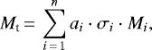 (1)
(1)
where ai is the molecular abundance of species i, σi is the electron impact ionisation cross-section(at 70 eV), and Mi is the corresponding fragmentation fraction. The following cross-sections are used: 2.275 (H2O), 2.441 (O2), 2.516 (CO), 3.521 (CO2) Å2 (Kim et al. 2014). As there is no available data in the literature for the ionisation cross-section of H2O2, its value is derived empirically. It is based on a linear correlation between the electron impact ionisation cross-section and polarisability (α), represented by a formula σ = 1.48 × α (Lampe et al. 1957; Bull et al. 2012). The polarisability of H2O2 is 1.73 Å3 (Johnson 2020), and the derived electron impact ionisation cross-section value for H2O2 is 2.5 Å2. The fragmentation pattern of H2O2 is adapted from Foner & Hudson (1962), where the contribution of fragments (peaks other than molecular ion) towards the total yield is 26%. The fragmentation patterns of other molecules relevant for this study are available in the NIST spectral database or previous works, but it should be noted that these are (slightly) dependent on the geometry of the experimental system (Kim et al. 2014). The use of these values allows us to solve Eq. (1) for ai (arbitrary units), which is proportional to the column density of each species (mol cm−2), i.
In the final step of the analysis, the calculated water abundance (in arbitrary units) is set equal to the known thickness of the deposited ice (9 × 10¹⁶ mol cm−2 or 90 ML assuming 1 × 10¹⁵ molecules per ML). Subsequently, the signals assigned to other species are converted with respect to the initial column density of water, allowing us to quantify their abundances for different UV fluences. The most significant uncertainty in this conversion is related to the uniformity of the ice thickness (±10%), and this value is taken into account when deriving abundances of photoproducts.
To translate the experimental results to environments with different astrochemical conditions, it is useful to describe the efficiency of the photoproduct formation as a molecular yield per amount of energy deposited in the ice. Hence, to calculate the fraction of absorbed photons (Iabs), the Beer-Lambert absorption law is used:
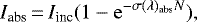 (2)
(2)
where Iinc is the incident UV photon fluence, σabs is the average photon absorption cross-section of the ice (H2O: 3.4 × 10⁻¹⁸ cm−2), and N is the ice column density (pure H2O experiments: 9 × 10¹⁶ mol cm−2) (Cruz-Diaz et al. 2014a). For calculations related to mixed ices, we used the following absorption cross-section values for CO2 and O2 : 6.7 × 10⁻¹⁹ cm−2 and 4.8 × 10⁻¹⁸ cm−2 (Cruz-Diaz et al. 2014b). For instance, after a UV irradiation of pure H2O ice with 4.8 × 10¹⁷ photons cm−2 (64 min), 1.3 × 10¹⁷ photons cm−2 are absorbed: each carry, on average, 9 eV of energy (Ligterink et al. 2015). Thus, after 64 min, a total energy of 1.2 × 10¹⁸ eV is deposited in the ice and each water molecule statistically absorbs 1.3 UV photons.
2.3 Overview of experiments
In this study, we focus on different ices starting with pure H2O, the primary constituent of interstellar ices. In a realistic interstellar ice, H2O molecules are expected to be mixed with CO2 (Öberg et al. 2007; Pontoppidan et al. 2008). Based on observations, the ratio of CO2/H2O in interstellar ices can vary from 12 to 40% (Boogert et al. 2015). Only in particular environments (Poteet et al. 2013; Isokoski et al. 2013) have pure CO2 ices been observed. Consequently, we also investigate the photochemistry of three different H2O:CO2 ice mixtures. Finally, as O2 may be formed asa side product of (non-energetic) water formation (see e.g. Cuppen et al. 2010; Minissale et al. 2014; Taquet et al. 2016), we also investigated H2O:CO2 ices enriched with O2. Once O2 is formed inan ice, it may start contributing to its overall chemical network. However, as the amount of molecular oxygen in the prestellar phase is not known, the recorded data for the O2 -containing ice are presented in the appendix. Table 1 summarises all performed experiments for pure H2O ice, H2O:CO2 ice mixtures (100:11, 100:22 and 100:44), and H2O:CO2:O2 (100:22:2). The assignment of the main photoproducts follows the H216O experiments, and the validity of these results is confirmed using H218O.
In addition to the H218O labeled experiments, another control experiment is performed to exclude error-prone results due to H2O background contamination. In this experiment, the substrate was exposed to H2O vapours above the sublimation point (190 K), which allows for the characterisation of the water deposited on the walls or ion optics.
The total and incremental UV fluence with which our ice samples are irradiated are representative of the different regions in the ISM. In the centre of a dark cloud, the photon fluence is estimated to be (3–30) × 1017 photons cm−2, considering cosmic ray induced secondary UV flux of (1–10) × 103 photons cm−2 s−1 and an average molecular cloud lifetime of up to 107 yr (Shen et al. 2004; Chevance et al. 2020). The UV fluence during a lifetime of a protoplanetary disc was modelled by Drozdovskaya et al. (2014), and, depending on the location within the disc, it varies between 1016 and 1026 photons cm−2.
Summary of the types of performed UV photolysis experiments.
3 Results
3.1 UV photolysis of H2O ice
The mass spectra obtained during the UV photolysis of pure H216O and H218O ices are shown in the upper and lower panels of Fig. 1, respectively. The bottom trace in each panel (black) is a reference mass spectrum that allows us to track changes from the initial composition of the ice. For H216O, the unprocessed signature includes peaks at m∕z = 16, 17, 18, and 19. Peaks at m∕z = 18 × n + 1, where n = 1, 2, and 3 represent protonated water clusters formed in the ablated plume, that is, these are not a reaction product from the UV irradiation, but result from the laser desorption pulse (Gudipati & Yang 2012).
After UV irradiation of the ice with a fluence of 6 × 10¹⁶ photons cm−2 (red trace, Fig. 1), new peaks appear at m∕z = 32, 34 in the H216O experiment (upper panel) and corresponding features at m∕z = 36 and 38 in the H218O experiment (lower panel). The mass shift of 4 atomic mass units (amu) reveals that the newly formed peaks represent species with two oxygen atoms. Considering the initial composition of the ice (pure H216O and H218O) and the reference mass spectra of possible photoproducts, the only species explaining these observations are O2 and H2O2. In addition, the mass peak at m∕z = 2 (for both isotopes) is increased, which must be due to the formation of molecular hydrogen (H2) in the ice.
The mass spectra clearly show that upon UV irradiation of water ice, O2 is formed in the solid state. The formation of H2 (m∕z = 2) and H2O2 (m∕z = 33, 34 in upper panel and m∕z = 37, 38 in lower panel) is observed simultaneously and it is important to note that the contribution of H2O2 towards mass peaks of O2 due to electron impact ionisation is negligible (Foner & Hudson 1962). As we probe the molecular plume before its interaction with the metal walls of the setup or its ion optics, the intensity of features representing O2+ and H2O2+ provides a firm base to quantify the formation of both photoproducts. This is shown as a function of UV fluence in Fig. 2. The abundances are calculated for multiple experiments with both isotopologues following the method described in Sect. 2.2. Subsequently, an exponential function was used to average the photoproduct yields from repeated experiments (for both isotopologues). The formation of O2 reaches its maximum of (7.6 ± 2.0) × 1014 molecules cm−2 at an incident photon fluence of 8.9 × 10¹⁷ photons cm−2. For the O2 formation relative to the current H2O abundance, we derive a maximum abundance of O2 /H2O to be (0.9 ± 0.2)%. The formation of closely related H2O2 is saturated at (1.1 ± 0.3) × 1015 molecules cm−2, which is converted to a relative maximum abundance of H2O2/H2O equal to (1.3 ± 0.3)% (see Appendix A for the water consumption during the experiments in this study).
The observed kinetic curves for O2 and H2O2 show the formation of both products in the early stages of photolysis. The photoproduct abundances reach a saturation level at a fluence of (4.8–8.9) × 1017 photons cm−2, the exposure dose that marks the equilibrium between formation and destruction routes.
To calculate the product formation efficiency per energy dose deposited in the ice, for each step of the photolysis, only the absorbed photons are considered. For each of the presented UV irradiation doses, the corresponding fraction of incident photons absorbed by the water ice is calculated using Eq. (2) as (26.0 ± 6.5)%. The largest uncertainty in the fraction of absorbed photons is based on the error bars related to the UV photon flux (25%). By calculating the yield for each UV dose, an upper limit was determined for the O2 formation in pure H2O ice as (1.3 ± 0.3) × 10−3 mol eV−1. A similar calculation was done for H2O2, which results in a maximum formation yield of (3.7 ± 0.9) × 10−3 mol eV−1.
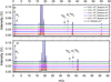 |
Fig. 1 LDPI TOF MS signals for a UV-irradiated H216O (upper panel) and H218O (lower panel) ice at 20 K for increasing photon fluence. The lowest trace in each plot shows the signal without UV irradiation. Besides H2O and its fragmentation pattern, these spectra reveal the presence of the photolysis products, H2, O2 and H2O2. In addition, protonated cluster ions (H2O)nH+ are seen to form in the desorption process (see text for details). |
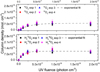 |
Fig. 2 Molecular abundances of species during the UV photolysis of H216O and H218O ices at 20 K as function of photon fluence: 16O2, 18O2 (upper panel) and H216O2, H218O2 (lower panel). The results from four separate experiments are shown. The initial ice thickness is (90 ± 10) ML. |
3.2 UV photolysis of H2O:CO2 (100:11, 100:22, and 100:44)
The mass spectra obtained during the UV photolysis of the H2O:CO2 = 100:11 ice mixture are shown in Fig. 3. The mass spectra for the 100:22 and 100:44 mixtures are presented in Appendix B.
The reference mass spectrum (Fig. 3, black trace), in addition to the previously described water signatures (see Fig. 2), includes the m∕z values characteristic for CO2, that is, m∕z = 12, 16, 28 and 44. Upon reaching a UV fluence of 6.0 × 10¹⁶ photons cm−2 (red trace), a number of new m∕z signals is observed. These signals are representative of the formation of H2O2 (m∕z = 34), H2 (m∕z = 2) and CO (m∕z = 28). The formation ofO2, at m∕z = 32, is detected simultaneously with H2CO (m∕z = 29, 30) and HCOOH (m∕z = 45 and 46). These assignments are based on the available chemical inventory in the ice and available reference mass spectra. The photoproduct formation is consistent with a decrease in the abundances of precursor species as discussed earlier (see Appendix A).
The mass spectra obtained during the photolysis of H2O:CO2 (100:22 and100:44) ices exhibit the formation of the same photoproducts, but at different relative intensities. This change is correlated with the relative increase in the abundance of CO2 which shifts the elemental balance towards carbon-containing species (CO, Appendix A), and also enhances the total oxygencontent.
The abundances of the identified photoproducts are derived for the three mixtures following the method described in Sect. 2.2. The formed product abundances for all mixtures are shown as a function of UV fluence in Fig. 4. The maximum formation yield of O2 reaches (2.4 ± 0.6) × 1014 molecules cm−2 (for the H2O:CO2 = 100:11 mixture), (3.4 ± 0.8) × 1014 molecules cm−2 (100:22), and (5.1 ± 1.2) × 1014 molecules cm−2 (100:44). The formation of H2O2 peaks at (8.5 ± 2.1) × 1014 (100:11), (3.8 ± 1.0) × 1014 molecules cm−2 (100:22), and (4.2 ± 1.0) × 1014 molecules cm−2 (100:44). It can be clearly seen that upon an increase in the abundance of CO2 in the mixtures with H2O, the maximum abundance of formed O2 increases with the amount of CO2 in the ice. An opposite behaviour is seen for H2O2 formation. Its upper limit abundance decreases, or stays constant, as the initial amount of CO2 in the ice mixture is increased.
In all mixtures, it is found that H2O depletes more efficiently, compared to pure H2O ice. The formation yields of the observed species are normalised to the current amount of H2O for each of the applied UV irradiation doses. Hence, even though the absolute yields of O2 and H2O2 in mixtures are slightly lower than in pure H2O ice photolysis, the relative abundance with respect to H2O is increased. For the 100:11 mixture, the relative abundance of O2 /H2O and H2O2/H2O reaches, respectively, (1.1 ± 0.3)% and (1.2 ± 0.3)%. For the 100:22 mixture, a relative abundance of O2 /H2O and H2O2/H2O reaches, respectively, (1.6 ± 0.4)% and (1.8 ± 0.4)%. In the 100:44 mixture, relative maximum abundances of O2 /H2O and H2O2/H2O are, respectively, (1.2 ± 0.3)% and (1.1 ± 0.3)%.
To compare the efficiency of photoproduct formation in the H2O:CO2 mixtures with the results obtained for the pure H2O ice, the peak abundances of products at corresponding UV fluences, have been converted to formation yields per energy dose deposited in the ice. To calculate the fraction of incident photons absorbed by the H2O:CO2 ice, we considered the ratio between ice constituents and their respective UV-absorption cross-sections. Consequently, for the H2O:CO2 (100:11, 100:22, 100:44) ice mixtures, the fraction of absorbed photons comprise (24.5 ± 6.1)%, (22.5 ± 5.6)% and (20.8 ± 5.2)%, respectively. Here, the uncertainty in the absorbed photons is again related to the UV flux throughout the photolysis. This results in the maximum formation yields of O2 equal to (6.1 ± 1.8) × 10−4 mol eV−1 (100:11), (9.7 ± 2.5) × 10−4 mol eV−1 (100:22), and (6.7 ± 2.1) × 10−4 mol eV−1 (100:44). The same calculation for H2O2 yields (3.2 ± 0.7) × 10−3 mol eV−1 (100:11), (1.5 ± 0.4) × 10−3 mol eV−1 (100:22), and (3.5 ± 1.0) × 10−3 mol eV−1 (100:44), respectively.
In addition to the mixtures studied above, where O2 is a product of photolysis of H2O:CO2, we investigated the photoevolution of an ice, which already includes O2 in the initial composition. The initial amount of O2, at a 2% level, is based on the results of modelling studies by Taquet et al. (2016). The quantitative analysis is presented in Appendix C.
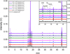 |
Fig. 3 LDPI TOF MS signals for a UV-irradiated H2O:CO2 ice at 100:11 ratio. The lowest trace in each panel shows the signal without UV irradiation. Peaks at m∕z = 18n + 1, where n = 1, 2 represent protonated water clusters formed upon laser desorption of water ice and do not contribute to the chemistry in the ice. The inset is a zoom on the intensity scale for the higher masses. |
 |
Fig. 4 Absolute molecular abundances of species during the UV photolysis of mixed ices: H2O:CO2 ice at 100:11 ratio (left panel), 100:22 (center panel), and 100:44 (right panel). Initial ice thickness is (90 ± 10) ML. |
4 Discussion
The results presented in the previous section allow us to discuss (i) the kinetic curves for O2 and H2O2 during UV irradiation of pure H2O ice at 20 K, (ii) the impact of including CO2 in the initial ice composition on (absolute and relative) photoproduct formation yields, and (iii) the presence of O2 in the initial mixture and the evolution of its abundance (and H2O2) as a function of UV fluence.
The formation of O2, H2O2 in pure H2O ice is observed immediately upon the onset of UV photolysis. Its efficiency is low, at a level of X/H2O ≈ 1%. To discuss the possible formation pathways, it is useful to recall the main photodissociation channels of H2O (Stief et al. 1975; Harich et al. 2000, 2001; van Harrevelt & van Hemert 2008; Slanger & Black 1982):
 (3)
(3)
 (4)
(4)
 (5)
(5)
 (6)
(6)
The potential of the newly formed free radicals as precursors for stable molecules is dictated by their abundance, relaxation rates, location within the ice, and diffusion abilities. The abundance of each fragment is given by the wavelength-dependent branching ratios following photodissociation. For H2O in the gas-phase, relative quantum yields following UV photodissociation within the used wavelength range consistently point to OH (in its ground or first excited state) and H as a dominant channel. This, however, can be different for the solid state (see Öberg et al. 2009a and Lucas et al. 2015 for CH3OH). It is also expected that the total effective photodissociation yield of radicals in the ice will be lower due to the recombination of fragments into the parent species. A detailed investigation of this process is required, but previous experimental studies show that the radical recombination in the water ice can decrease the photodissociation yield by 43–72%, compared to the gas phase (Mason et al. 2006; Cruz-Diaz et al. 2014a; Kalvāns 2018).
The location of the photodissociation event within the ice is important; combined with the temperature of the ice, it determines the diffusion abilities of the fragments (Andersson et al. 2006; Andersson & van Dishoeck 2008; Arasa et al. 2010). In particular, if H and OH are formed from photodissociation in the top layers of the ice (~3 ML), both radicals can travel up to a few tens of angstroms within (or on top of) the ice (Andersson & van Dishoeck 2008). However, the average distance travelled by H and OH fragments in the ice is 8 Å and 1 Å, respectively. In a realistic scenario, free radicals are formed randomly throughout the ice and can be formed in two different chemical environments: at the ice and vacuum interface on the surface (including pores) and within the ice bulk. In our experiments, the ice thickness (90 ML) was chosen to maximise the contribution of the radicals created in the ice bulk; however, the exact ratio of radicals created in the bulk versus the surface (and pores) is not known. The presence of such a large parameter space significantly complicates the interpretation of our data. Nevertheless, some important observations can be made.
Under the assumption that photodissociation of H2O mainly leads to the formation of H and OH (in the ground or excited states), the formation of H2O2 and H2 can be easily accounted for by radical recombination reactions of OH+OH and H+H. However, as formation of O2 can be observed already during the early stages of irradiation, simultaneously with the formation of H2O2 (see Fig. 2), the involved O2 formation routes must be connected to those of H2O2 and H2 and involve the direct products of H2O photodissociation. Hence, we suggest that O radicals are present in the ice directly upon water photodissociation (reactions 5 and 6). The formation of O(1D) via reaction (5) was demonstrated experimentally as a primary process upon photolysis of ASW (UV photolysis with 157 nm at 90 K) by Hama et al. (2009a). This radical can either proceed to react with water via O(1D)+H2O → 2OH (Sayós et al. 2001), or relax to its ground state and react with OH to form O2 via O(3P) + OH → O2 + H (Hama et al. 2010). Channel (6) has not been observed experimentally; however, its contributionis not excluded as the Ly-alpha photons in our spectrum are capable of dissociating water into O(3P) (van Harrevelt & van Hemert 2008). During later stages of photolysis, secondary reaction channels, such as photodissociation of OH or recombination of OH radicals can contribute towards the formation of O(3P), and consequently, O2 (Hama et al. 2009b, 2010).
It is also important to mention that the photodepletion of water is below ~10%. Such inefficient depletion, even for a relatively large number of absorbed photons per H2O molecule (i.e. 4–5; see Sect. 3.1), suggests that pure water ice is resilient to UV irradiation, in part due to efficient conversion of the formed products back into H2O.
The photolysis of H2O:CO2 ice mixtures provides additional radical precursors via the following pathways (Slanger & Black 1978; Kinugawa et al. 2011):
 (7)
(7)
 (8)
(8)
The addition of CO2 in the ice results in a decreased absolute formation yield of O2 and H2O2 in comparison to pure H2O ice photolysis (see Figs. 2 and 4). This could be due to the lower initial abundance of water (90 ML) and/or CO2 photodissociation products providing reactive radicals leading to competing photoproducts. Indeed, interactions of OH radicals with CO (produced by photodissociation of CO2) lead to the (re)formation of CO2 (Hama et al. 2010; Ioppolo et al. 2011). Consistently with fewer OH radicals available, we observe a reduced amount of formed H2O2. In addition, if O radicals are present via water photodissociation (see point i) in the discussion), these fragments can also react with CO, to reform CO2, constraining the absolute formation of O2.
Increasing the relative CO2 abundance (H2O:CO2 from 100:11 to 100:44) leads to a proportional increase in the O2 formation. The maximum formation yield of O2 is increased from (2.4 ± 0.6) × 1014 molecules cm−2 to (5.1 ± 1.2) × 1014 molecules cm−2 for H2O:CO2 mixtures with a ratio of 100:11 and 100:44, respectively (see Fig. 4). This is in line with the increased production of O atoms, via photodissociation of CO2 in the ice and formation of O2 following O+OH and O+O interactions. With more initial CO2, the formation of H2O2 becomes less efficient, which could be simply due to fewer OH radicals available in the ice and the competitive reaction of CO + OH → CO2.
The absolute yields of O2 and H2O2 during UV photolysis of mixed ices (H2O:CO2) are lower compared to pure H2O ice, however, the relative abundances of O2 /H2O increase. This is due to a more significant photoconversion of H2O molecules toother species.
The analysis of the most complex H2O:CO2:O2 ice mixture provides hints for more efficient formation pathways towards O2 and H2O2 (see Appendix C). In this mixture, in addition to the previously described fragments, O radicals are available directly upon photodissociation of O2 (Lambert et al. 2004):
 (9)
(9)
 (10)
(10)
At the early stages of photolysis, the formation efficiency of both O2 and H2O2 (mol eV−1) is an order of magnitude higher compared to other mixtures or pure water ice. The interpretation of such a result should be performed carefully, as here a precursor is included that in fact is the reaction product the experiment is aiming at. It is found, however, that the maximum abundance observed during the photolysis cannot be accounted for by the initial O2 injection (Fig. C.2). The increased formation yield hints for additional chemical mechanisms from the pathways discussed above. These are most likely associated with the presence of a highly reactive radical, O(1D). The increased formation of O2 might indeed be partially due to O(1D) radicals produced via the dissociation of O2, reacting with CO2, H2O or their photodissociation products (Wen & Thiemens 1993; Sayós et al. 2000). A significantly higher abundance (compared to other mixtures) is also observed for H2O2. This could be due to a barrierless reaction of O(1D) + H2O → 2OH, which provides precursor species for the typical radical recombination reaction (OH + OH) leading to H2O2 (Sayós et al. 2001). It is also found that H2O:CO2:O2 ice mixture is the only ice studied here, where efficient formation of H2 is not observed. This suggests that H atoms are consumed via reactions with other ice constituents: CO, O, OH, or O2.
5 Astrophysical implications
The majority of water in the ISM exists in the solid state and is formed via atom addition reactions on the grains in the dense molecular clouds (Lamberts et al. 2013; Linnartz et al. 2015; van Dishoeck et al. 2021). In addition to H2O molecules produced by the hydrogenation of accreting O atoms (O + H → OH and OH + H/H2 → H2O), other simple molecules are formed during this stage that contribute to the bulk of observed H2O-rich ices. These molecules include NH3 and CH4, produced by the hydrogenation of N and C atoms, respectively, as well as CO2, produced through the interaction of accreting CO molecules with OH radicals (Fedoseev et al. 2015; Qasim et al. 2020; Hama et al. 2010; Ioppolo et al. 2011). Simultaneously, depending on the local physical environment, an O2 ice reservoir can accumulate (Taquet et al. 2016). Towards the end of the accretion stage in a dense molecular cloud, the increase in chemical complexity of the icy mantles is driven by various types of energetic processing (e.g. cosmic rays, X-rays, UV photons). Later, the chemically enriched icy mantles become part of the material from which a young star, its surrounding planets and other celestial bodies, such as comets, are made from. In fact, the transfer of ices from dark clouds to protoplanetary discs and comets was discussed by Taquet et al. (2016), which showed that the chemical composition of the ices along the comet formation sequence is preserved.
To place our experiments in an astronomical context, Fig. 5 (left panel) shows the relative abundance of O2 /H2O for the four studied ice compositions: pure H2O and H2O:CO2 (100:11, 100:22, 100:44). In addition, the abundances detected in the cometary comae of 67P (3.1 ± 1.1)%) and 1P (3.7 ± 1.7)% are marked. In the experiments we show that during the photolysis of pure H2O ice, the O2 /H2O ratio can increase up to a level (0.9 ± 0.2)%, roughly three-four times less than the detected abundances in the cometary comea. For ice mixtures more adequately representing icy mantles (H2O:CO2), the O2 /H2O abundance increases with an increasing initial amount of CO2, up to (1.6 ± 0.4)% for the H2O:CO2 (100:22) ice.This value is within a of factor 2 in the range of the cometary abundances. It is expected that other abundant constituents of interstellar ices may also have an impact on relative formation of O2 /H2O. As an example, the presence of CO can lead to a decrease in the number of available H atoms in the ice, as its successive hydrogenations lead to efficient formation ofH2CO and CH3OH (Watanabe & Kouchi 2002). Subsequently, it would inhibit the recombination of water (OH + H), leaving OH radicals that could change the O2 /H2O ratio. Dedicated astrochemical modelling is needed to understand how these processes combine with each other.
With regard to species that are chemically related, the non-detection of O3 and HO2 in our experiments is consistent with low cometary and ISM measurements. The abundance ratio of HO2/O2 for both the 67P and ρ Oph A is 2 × 10⁻³ (Bieler et al. 2015; Parise et al. 2012), while for O3 there is only an upper limit abundance with respect to O2 at 2 × 10⁻⁵.
The key discrepancy between our experiments and cometary observations is in the abundance of H2O2. Its formation during UV photolysis is at a similar level to O2, which is two orders of magnitude above the observed values (Bieler et al. 2015). An explanation for this might be in an efficient dismutation of H2O2, upon thermal desorption of the water ice as demonstrated by Dulieu et al. (2017). Based on Smith et al. (2011), H2O2 is expected to be present in the interstellar ices at an abundance of (9 ± 4)% with respect to H2O and to survive the transfer to the nucleus of the comet. Subsequently, when the comet thermally releases species trapped within the cometary ice, including H2O2, hydrogen peroxide undergoes a dismutation via 2H2O2 → 2H2O + O2, which is found to produce O2 /H2O yields from 1 to 10% (Dulieu et al. 2017).
Our experiments are set up such that the abundances we record in the gas phase are a direct measure of the ices. The same may not be the case for the gases observed in the comae around comets 1P and 67P. Therefore, dismutation producing O2 gas from H2O2 gas could be a contributing factor to the measured abundance of O2 in the comets. If O2 and H2O2 ices are produced in similar amounts in the cometary ices (similar to the results from our work), and assuming that all H2O2 is processed into O2 (the H2O2 abundance is two orders of magnitude below O2 in the comet 67P), then the observed abundance of O2 in the cometary comae may be higher than when it was still in the cometary ice (see also Dulieu et al. 2017; Mousis et al. 2016). If we apply this logic to the experimental yields derived here, then the O2 abundances are shifted up by the contribution from the H2O2 molecules (two H2O2 molecules are converted into one O2). Taking this into account, the experimental values for O2 abundance (in the gas-phase) for a UV fluence of just under 2 × 10¹⁸ photons cm−2 and an icemixture of H2O:CO2 (100:22) would fall within the observed abundance limits in both comets (see Fig. 5, right panel).
For the O2 -enriched ices, an increase in the O2 /H2O ratio is seen for all non-zero UV fluences. It varies between ~3% and ~7%, with the maximum yield at a relatively low UV fluence (based on Fig. C.2). This corresponds to an increase in O2 /H2O abundance by a factor of 1.5–3.5, relatively to the initial O2 amount. Following this, it can be argued that the icy material in comets 1P and 67P could have started out (prior to the pre-solar nebula-stage) with a smaller O2 /H2O ice ratio than seen today. Subsequently, during evolution and if subjected to UV photons (or possibly other energetic processing), the initial ratio could have increased by a factor 1.5–3.5, to explain the ratio that is derived from the Rosina and Giotto missions.
It should be noted that UV photolysis is not the only process that affects the composition of the interstellar ices. Other sources of chemical diversity include high-energy particles, X-rays, cosmic rays (CR) themselves, or CR-triggered avalanches of secondary electrons. In the last two decades, the effects of these processes have been investigated via experimentsand astrochemical models (Gomis et al. 2004; Zheng et al. 2006a; Mousis et al. 2016, 2018; Eistrup & Walsh 2019; Teolis et al. 2017; Shingledecker et al. 2018, 2019; Notsu et al. 2021). These experimental and modelling findings, combined with our novel results, which may (largely) explain the observed cometary O2 /H2O ratios, stress the importance of precise chemical modelling. The work presented here now provides explicit values as input parameters.
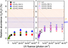 |
Fig. 5 Striped areas represent relative O2/H2O abundances detected in cometary comae of 67P and 1P from Rubin et al. (2019). The data points represent the laboratory experiments presented here. Left panel: molecular abundance of O2 normalised to the amount of H2O at each UV dose for different initial compositions of the ice. Right panel: molecular abundance of O2 enhanced by the decomposition of H2O2 (see text fordetails). |
6 Conclusions
LDPI TOF MS was applied to quantify the formation of O2 during UV irradiation of simple interstellar ice analogues (H2O, H2O:CO2 and H2O:CO2:O2) at 20 K. The main results are as follows.
- 1.
For a UV photon fluence representative of dense molecular clouds and innermost regions of protoplanetary discs (~1018 photons cm−2), UV irradiation of porous amorphous H2O ice at 20 K leads to formation of O2 and H2O2 in the solid state. The maximum abundances of (O2/H2O) and H2O2/H2O are equal to (0.9 ± 0.2)% and (1.3 ± 0.3)%, respectively.
- 2.
The mixing of H2O with CO2 ice with the ratios 100:11, 100:22, and 100:44 results in an increased relative formation of O2/H2O, with a maximum value of (1.6 ± 0.4)% for the 100:22 mixture. This also shows that CO2 is involved in the formation of molecular oxygen.
- 3.
The maximum formation efficiency of O2 and H2O2 per energy unit deposited in the pure H2O ice at 20 K are: (1.3 ± 0.3) × 10−3 mol eV−1 and (3.7 ± 1.0) × 10−3 mol eV−1. These yields are similar for the H2O:CO2 mixtures; for O2 it is (9.7 ± 0.4) × 10−4 mol eV−1, and for H2O2 it is (3.5 ± 0.9) × 10−3 mol eV−1. However, the corresponding maximum photoproduct formation efficiency in the H2O:CO2:O2 mixture are almost an order of magnitude higher; for O2 it is (1.1 ± 0.3) × 10−2 mol eV−1 , and for H2O2 it is (1.6 ± 0.4) × 10−2 mol eV−1. This is without the contribution of the O2 already present in the mixture.
- 4.
The abundances of O2/H2O found in our experiments are sufficient to account for at least part of the observed cometary abundances.
This work demonstrates the potential of MATRI2CES to investigate the photochemical evolution of interstellar ices analogues, including the infrared-inactive species, upon UV photolysis at low temperature.
Acknowledgements
The authors would like to acknowledge T. Hama for his thorough referee report which improved the quality of this article. M.B. and H.L. acknowledge the European Union (EU) and Horizon 2020 funding awarded under the Marie Sk?odowska-Curie action to the EUROPAH consortium (grant number 722346) as well as NOVA 5 funding. Recent support through INTERCAT is acknowledged as well. Additional funding has been realized through a NWO-VICI grant. G.F. also acknowledges financial support from the Russian Ministry of Science and Higher Education via the State Assignment Contract FEUZ-2020-0038. J.T.v.S. is supported by the Dutch Astrochemistry II program of the Netherlands Organization for Scientific Research (648.000.025). The authors thank A.G.G.M. Tielens for constructive discussions and remarks.
Appendix A Abundance of H2O and CO during UV photolysis
The photodepletion of water was derived for all ices investigated in this study and is shown in Fig. A.1. For the pure H2O ice, the depletion was below the uncertainty related to the initial ice thickness; hence, it was calculated based on the abundances of formed photoproducts. The total abundance of O2 and H2O2 reached ~2 × 10¹⁵ molecules cm−2. Under the assumption that each of these species requires two H2O molecules, the lower limit of water consumption was derived to be (4.0) × 1015 molecules cm−2, which is 4% of the initial column density of the ice.
The formation of CO was derived for all mixed ices investigated in this study, shown in Fig. A.2. Towards the end of UV photolysis, CO was the dominant photoproduct, with a maximum yield in the H2O:CO2:O2 (100:22:2) mixture.
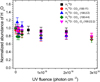 |
Fig. A.1 Molecular abundance of H2O normalised to its initial amount as a function of UV photon fluence for different initial compositions of the ice. |
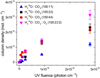 |
Fig. A.2 Molecular abundance of CO as a function of UV photon fluence for different initial compositions of the ice. |
Appendix B UV photolysis of H2O:CO2 (100:22 and 100:44)
The mass spectra obtained during the UV photolysis of the H2O:CO2 = 100:22 and H2O:CO2 = 100:44 icemixtures are shown in Fig. B.1 and B.2.
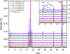 |
Fig. B.1 LDPI TOF MS signals for a UV-irradiated H2O:CO2 ice at 100:22 ratio. The lowest trace in each panel shows the signal without UV irradiation. Peaks at m∕z = 18⋅n+1, where n = 1, 2 represent protonated water clusters formed upon laser desorption of water ice and do not contribute to the chemistry in the ice. The inset shows a zoomed-in image of the intensity scale for the higher masses. |
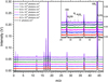 |
Fig. B.2 LDPI TOF MS signals for a UV-irradiated H2O:CO2 ice at 100:44 ratio. The lowest trace in each panel shows the signal without UV irradiation. Peaks at m∕z = 18⋅n+1, where n = 1, 2 represent protonated water clusters formed upon laser desorption of water ice and do not contribute to the chemistry in the ice. The inset shows a zoomed-in image of the intensity scale for the higher masses. |
Appendix C UV photolysis of H2O:CO2:O2 (100:22:2)
The mass spectra resulting from the UV photolysis of an H2O:CO2:O2 (100:22:2) mixture are shown in Fig. C.1. The reference mass spectrum (black trace), in addition to the previously described signatures of H2O and CO2, also shows the m∕z values corresponding to the initialO2, at m∕z = 16 and 32.
After UV irradiation of the ice with a fluence of 6 × 10¹⁶ photons cm−2 (red trace, Fig. C.1), new peaks appear at m∕z = 33, 34, and the intensityof features at m∕z = 28, 29, 32, and 45 increases. This is representative of the formation of H2O2, CO, H2CO, O2 and HCOOH. In order to quantify the formation yields of CO and O2, the signals corresponding to the initial abundances of CO2 (a fragment overlapping with CO at m∕z = 28) and O2 are subtracted, allowing us to trace the contribution from the newly formed molecules. We note that no H2 signal is observed until a high UV fluence of 1.9 × 10¹⁸ photons cm−2 is reached.
The abundances of identified photoproducts are calculated following the method described in Sect. 2.2. and are presented in Fig. C.2. The O2 abundance increases, reaching (4.5 ± 1.1) × 1015 molecules cm−2. Upon reaching a UV fluence of 2.4 × 10¹⁷ photons cm−2, the O2 destruction efficiency matches the O2 formation rate and starts to dominate at higher UV fluence. At a fluence of 3.7 × 10¹⁸ photons cm−2, the O2 abundance continues to decrease, with a final yield below the initial O2 abundance.
The formation of H2O2 in this mixture follows a trend similar to O2. Its abundance reaches a maximum of (3.5 ± 0.9) × 1015 molecules cm−2 at 2.4 × 10¹⁷ photons cm−2. Upon longer irradiation, its abundance decreases to (1.7 ± 0.4) × 1015 molecules cm−2 at 3.7 × 10¹⁸ photons cm−2.
The quantified consumption of H2O (Appendix A) is used to derive an upper limit on the relative photoproduct formation (X/H2O) during the photolysis of H2O:CO2:O2 ices. The upper limit of the relative abundance of (O2 /H2O) is calculated to be (6.9 ± 1.6)%, and the corresponding value for (H2O2/H2O) is (5.4 ± 1.4)%.
The H2O:CO2:O2 (100:22:2) ice at each UV dose absorbs (25.7 ± 7.2)% of incident photons. Consequently, the formation yields of O2 and H2O2 reach their maxima equal to (1.1 ± 0.3) × 10−2 mol. eV−1 and (1.6 ± 0.3) × 10−2 mol. eV−1, respectively.In comparison to the photolysis of pure water ice and mixtures with CO2, the formation efficiency (in mol. eV−1) of both products in this mixture is higher by one order of magnitude.
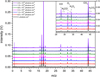 |
Fig. C.1 LDPI TOF MS signals for a UV-irradiated H2O:CO2:O2 ice at 100:22:2 ratio at 20 K. The lowest graph shows the signal without UV irradiation. The inset shows a zoomed-in image of the intensity scale for the higher masses. Peaks at m∕z = 18⋅n+1, where n = 1, 2 represent protonated water clusters formed upon laser desorption of water ice and do not contribute to the chemistry in the ice. |
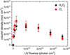 |
Fig. C.2 Absolute molecular abundances of species during the UV photolysis of mixed ices: H2O:CO2:O2 ice at 100:22:2 ratio. Initial ice thickness is (90 ±10) ML. |
References
- Andersson, S., & van Dishoeck, E. F. 2008, A&A, 491, 907 [NASA ADS] [CrossRef] [EDP Sciences] [Google Scholar]
- Andersson, S., Al-Halabi, A., Kroes, G.-J., & van Dishoeck, E. F. 2006, J. Chem. Phys., 124, 064715 [NASA ADS] [CrossRef] [Google Scholar]
- Arasa, C., Andersson, S., Cuppen, H. M., van Dishoeck, E. F., & Kroes, G. J. 2010, J. Chem. Phys., 132, 184510 [NASA ADS] [CrossRef] [Google Scholar]
- Bar-Nun, A., Herman, G., Rappaport, M., & Mekler, Y. 1985, Surf. Sci., 150, 143 [NASA ADS] [CrossRef] [Google Scholar]
- Baragiola, R. A., Atteberry, C. L., Dukes, C. A., Famá, M., & Teolis, B. D. 2002, Nucl. Instr. Methods Phys. R. B, 193, 720 [NASA ADS] [CrossRef] [Google Scholar]
- Baratta, G. A., & Palumbo, M. E. 1998, J. Opt. Soc. Am. A, 15, 3076 [Google Scholar]
- Bieler, A., Altwegg, K., Balsiger, H., et al. 2015, Nature, 526, 678 [Google Scholar]
- Bockelée-Morvan, D., Lis, D. C., Wink, J. E., et al. 2000, A&A, 353, 1101 [Google Scholar]
- Boogert, A. C. A., Pontoppidan, K. M., Knez, C., et al. 2008, ApJ, 678, 985 [Google Scholar]
- Boogert, A. C. A., Gerakines, P. A., & Whittet, D. C. B. 2015, ARA&A, 53, 541 [Google Scholar]
- Brown, W., Augustyniak, W., Simmons, E., et al. 1982, Nucl. Instr. Methods Phys. R, 198, 1 [Google Scholar]
- Bulak, M., Paardekooper, D. M., Fedoseev, G., & Linnartz, H. 2020, A&A, 636, A32 [NASA ADS] [CrossRef] [EDP Sciences] [Google Scholar]
- Bull, J. N., Harland, P. W., & Vallance, C. 2012, J. Phys. Chem. A, 116, 767 [NASA ADS] [CrossRef] [Google Scholar]
- Castellanos, P., Candian, A., Zhen, J., Linnartz, H., & Tielens, A. G. G. M. 2018, A&A, 616, A166 [NASA ADS] [CrossRef] [EDP Sciences] [Google Scholar]
- Chevance, M., Kruijssen, J. M. D., Hygate, A. P. S., et al. 2020, MNRAS, 493, 2872 [NASA ADS] [CrossRef] [Google Scholar]
- Chuang, K. J., Fedoseev, G., Qasim, D., et al. 2018, A&A, 617, A87 [NASA ADS] [CrossRef] [EDP Sciences] [Google Scholar]
- Cruz-Diaz, G. A., Muñoz Caro, G. M., Chen, Y. J., & Yih, T. S. 2014a, A&A, 562, A119 [NASA ADS] [CrossRef] [EDP Sciences] [Google Scholar]
- Cruz-Diaz, G. A., Muñoz Caro, G. M., Chen, Y. J., & Yih, T. S. 2014b, A&A, 562, A120 [NASA ADS] [CrossRef] [EDP Sciences] [Google Scholar]
- Cruz-Diaz, G. A., Martín-Doménech, R., Moreno, E., Muñoz Caro, G. M., & Chen, Y.-J. 2018, MNRAS, 474, 3080 [Google Scholar]
- Cuppen, H. M., Ioppolo, S., Romanzin, C., & Linnartz, H. 2010, PCCP, 12, 12077 [CrossRef] [Google Scholar]
- Drozdovskaya, M. N., Walsh, C., Visser, R., Harsono, D., & van Dishoeck, E. F. 2014, MNRAS, 445, 913 [NASA ADS] [CrossRef] [Google Scholar]
- Dulieu, F., Minissale, M., & Bockelée-Morvan, D. 2017, A&A, 597, A56 [NASA ADS] [CrossRef] [EDP Sciences] [Google Scholar]
- Eistrup, C., & Walsh, C. 2019, A&A, 621, A75 [NASA ADS] [CrossRef] [EDP Sciences] [Google Scholar]
- Fedoseev, G., Ioppolo, S., Zhao, D., Lamberts, T., & Linnartz, H. 2015, MNRAS, 446, 439 [NASA ADS] [CrossRef] [Google Scholar]
- Fillion, J.-H., Dupuy, R., Féraud, G., et al. 2021, A&A, submitted [arXiv:2103.15435] [Google Scholar]
- Foner, S. N., & Hudson, R. L. 1962, J. Chem. Phys., 36, 2676 [NASA ADS] [CrossRef] [Google Scholar]
- Gerakines, P. A., Schutte, W. A., & Ehrenfreund, P. 1996, A&A, 312, 289 [NASA ADS] [Google Scholar]
- Gomis, O., Leto, G., & Strazzulla, G. 2004, A&A, 420, 405 [NASA ADS] [CrossRef] [EDP Sciences] [Google Scholar]
- Gudipati, M. S., & Yang, R. 2012, ApJ, 756, L24 [Google Scholar]
- Hama, T., Yabushita, A., Yokoyama, M., Kawasaki, M., & Watanabe, N. 2009a, J. Chem. Phys., 131, 114510 [NASA ADS] [CrossRef] [Google Scholar]
- Hama, T., Yabushita, A., Yokoyama, M., Kawasaki, M., & Watanabe, N. 2009b, J. Chem. Phys., 131, 114511 [NASA ADS] [CrossRef] [Google Scholar]
- Hama, T., Yokoyama, M., Yabushita, A., & Kawasaki, M. 2010, J. Chem. Phys., 133, 104504 [NASA ADS] [CrossRef] [Google Scholar]
- Harich, S. A., Hwang, D. W., Yang, X., et al. 2000, J. Chem. Phys., 113, 10073 [CrossRef] [Google Scholar]
- Harich, S. A., Yang, X. F., Yang, X., van Harrevelt, R., & van Hemert, M. C. 2001, Phys. Rev. Lett., 87, 263001 [NASA ADS] [CrossRef] [Google Scholar]
- Ioppolo, S., Cuppen, H. M., Romanzin, C., van Dishoeck, E. F., & Linnartz, H. 2008, ApJ, 686, 1474 [NASA ADS] [CrossRef] [Google Scholar]
- Ioppolo, S., Cuppen, H. M., Romanzin, C., van Dishoeck, E. F., & Linnartz, H. 2010, PCCP, 12, 12065 [NASA ADS] [CrossRef] [Google Scholar]
- Ioppolo, S., van Boheemen, Y., Cuppen, H. M., van Dishoeck, E. F., & Linnartz, H. 2011, MNRAS, 413, 2281 [NASA ADS] [CrossRef] [Google Scholar]
- Isokoski, K., Poteet, C. A., & Linnartz, H. 2013, A&A, 555, A85 [NASA ADS] [CrossRef] [EDP Sciences] [Google Scholar]
- Jenniskens, P., Blake, D. F., & Kouchi, A. 1998, in ASSL, 227, Solar SystemIces, eds. B. Schmitt, C. de Bergh, & M. Festou (Dordrecht: Springer), 139 [Google Scholar]
- Jo, S. K., & White, J. M. 1991, J. Chem. Phys., 94, 5761 [NASA ADS] [CrossRef] [Google Scholar]
- Johnson, R. E. 1991, J. Geophys. Res., 96, 17553 [NASA ADS] [CrossRef] [Google Scholar]
- Johnson, III, R. D. 2020, NIST Computational Chemistry Comparison and Benchmark Database; NIST Standard Reference Database Number 101, http://cccbdb.nist.gov [Google Scholar]
- Johnson, R. E., & Quickenden, T. I. 1997, J. Geophys. Res., 102, 10985 [NASA ADS] [CrossRef] [Google Scholar]
- Kalvāns, J. 2018, MNRAS, 478, 2753 [CrossRef] [Google Scholar]
- Kim, Y. K., Irikura, K. K., Rudd, M. E., & Ali, M. A. 2014, Electron-Impact Ionization Cross Section for Ionization and Excitation Database (version 3.0) [Google Scholar]
- Kimmel, G. A., & Orlando, T. M. 1995, Phys. Rev. Lett., 75, 2606 [NASA ADS] [CrossRef] [Google Scholar]
- Kinugawa, T., Yabushita, A., Kawasaki, M., Hama, T., & Watanabe, N. 2011, PCCP, 13, 15785 [NASA ADS] [CrossRef] [Google Scholar]
- Kofman, V., He, J., Loes ten Kate, I., & Linnartz, H. 2019, ApJ, 875, 131 [NASA ADS] [CrossRef] [Google Scholar]
- Lambert, H. M., Dixit, A. A., Davis, E. W., & Houston, P. L. 2004, J. Chem. Phys., 121, 10437 [CrossRef] [Google Scholar]
- Lamberts, T., Cuppen, H. M., Ioppolo, S., & Linnartz, H. 2013, PCCP, 15, 8287 [NASA ADS] [CrossRef] [Google Scholar]
- Lampe, F., Franklin, J., & Field, F. 1957, J. Am. Chem. Soc., 79, 6129 [CrossRef] [Google Scholar]
- Larsson, B., & Liseau, R. 2017, A&A, 608, A133 [NASA ADS] [CrossRef] [EDP Sciences] [Google Scholar]
- Larsson, B., Liseau, R., Pagani, L., et al. 2007, A&A, 466, 999 [NASA ADS] [CrossRef] [EDP Sciences] [Google Scholar]
- Leto, G., & Baratta, G. A. 2003, A&A, 397, 7 [NASA ADS] [CrossRef] [EDP Sciences] [Google Scholar]
- Ligterink, N. F. W., Paardekooper, D. M., Chuang, K.-J., et al. 2015, A&A, 584, A56 [NASA ADS] [CrossRef] [EDP Sciences] [Google Scholar]
- Linnartz, H., Ioppolo, S., & Fedoseev, G. 2015, Int. Rev. Phys. Chem., 34, 205 [Google Scholar]
- Liseau, R., Goldsmith, P. F., Larsson, B., et al. 2012, A&A, 541, A73 [NASA ADS] [CrossRef] [EDP Sciences] [Google Scholar]
- Lucas, M., Liu, Y., Bryant, R., Minor, J., & Zhang, J. 2015, Chem. Phys. Lett., 619, 18 [NASA ADS] [CrossRef] [Google Scholar]
- Luspay-Kuti, A., Mousis, O., Lunine, J. I., et al. 2018, Space Sci. Rev., 214, 115 [NASA ADS] [CrossRef] [Google Scholar]
- Mason, N. J., Dawes, A., Holtom, P. D., et al. 2006, Far. Disc., 133, 311 [NASA ADS] [CrossRef] [Google Scholar]
- Minissale, M., Congiu, E., & Dulieu, F. 2014, J. Chem. Phys., 140, 074705 [NASA ADS] [CrossRef] [Google Scholar]
- Miyauchi, N., Hidaka, H., Chigai, T., et al. 2008, Chem. Phys. Lett., 456, 27 [CrossRef] [Google Scholar]
- Mousis, O., Ronnet, T., Brugger, B., et al. 2016, ApJ, 823, L41 [Google Scholar]
- Mousis, O., Ronnet, T., Lunine, J. I., et al. 2018, ApJ, 858, 66 [NASA ADS] [CrossRef] [Google Scholar]
- Müller, B., Giuliano, B. M., Bizzocchi, L., Vasyunin, A. I., & Caselli, P. 2018, A&A, 620, A46 [NASA ADS] [CrossRef] [EDP Sciences] [Google Scholar]
- Notsu, S., van Dishoeck, E. F., Walsh, C., Bosman, A. D., & Nomura, H. 2021, A&A, 650, A180 [NASA ADS] [CrossRef] [EDP Sciences] [Google Scholar]
- Oba, Y., Miyauchi, N., Hidaka, H., et al. 2009, ApJ, 701, 464 [NASA ADS] [CrossRef] [Google Scholar]
- Öberg, K. I., Fraser, H. J., Boogert, A. C. A., et al. 2007, A&A, 462, 1187 [NASA ADS] [CrossRef] [EDP Sciences] [Google Scholar]
- Öberg, K. I., Garrod, R. T., van Dishoeck, E. F., & Linnartz, H. 2009a, A&A, 504, 891 [NASA ADS] [CrossRef] [EDP Sciences] [Google Scholar]
- Öberg, K. I., Linnartz, H., Visser, R., & van Dishoeck, E. F. 2009b, ApJ, 693, 1209 [Google Scholar]
- Paardekooper, D. M., Bossa, J. B., Isokoski, K., & Linnartz, H. 2014, Rev. Sci. Instrum., 85, 104501 [NASA ADS] [CrossRef] [Google Scholar]
- Paardekooper, D. M., Fedoseev, G., Riedo, A., & Linnartz, H. 2016, A&A, 596, A72 [NASA ADS] [CrossRef] [EDP Sciences] [Google Scholar]
- Parise, B., Bergman, P., & Du, F. 2012, A&A, 541, L11 [NASA ADS] [CrossRef] [EDP Sciences] [Google Scholar]
- Pontoppidan, K. M., Boogert, A. C. A., Fraser, H. J., et al. 2008, ApJ, 678, 1005 [NASA ADS] [CrossRef] [Google Scholar]
- Poteet, C. A., Pontoppidan, K. M., Megeath, S. T., et al. 2013, ApJ, 766, 117 [NASA ADS] [CrossRef] [Google Scholar]
- Qasim, D., Fedoseev, G., Chuang, K. J., et al. 2020, Nat. Astr., 4, 781 [NASA ADS] [CrossRef] [Google Scholar]
- Rubin, M., Altwegg, K., van Dishoeck, E. F., & Schwehm, G. 2015, ApJ, 815, L11 [NASA ADS] [CrossRef] [Google Scholar]
- Rubin, M., Altwegg, K., Balsiger, H., et al. 2019, MNRAS, 489, 594 [Google Scholar]
- Satorre, M. Á., Domingo, M., Millán, C., et al. 2008, Planet. Space Sci., 56, 1748 [NASA ADS] [CrossRef] [Google Scholar]
- Sayós, R., Oliva, C., & González, M. 2000, J. Chem. Phys., 113, 6736 [CrossRef] [Google Scholar]
- Sayós, R., Oliva, C., & González, M. 2001, J. Chem. Phys., 115, 8828 [CrossRef] [Google Scholar]
- Shen, C. J., Greenberg, J. M., Schutte, W. A., & van Dishoeck, E. F. 2004, A&A, 415, 203 [NASA ADS] [CrossRef] [EDP Sciences] [Google Scholar]
- Shingledecker, C. N., Tennis, J., Le Gal, R., & Herbst, E. 2018, ApJ, 861, 20 [Google Scholar]
- Shingledecker, C. N., Vasyunin, A., Herbst, E., & Caselli, P. 2019, ApJ, 876, 140 [Google Scholar]
- Sieger, M. T., Simpson, W. C., & Orlando, T. M. 1998, Nature, 394, 554 [NASA ADS] [CrossRef] [Google Scholar]
- Slanger, T. G., & Black, G. 1978, J. Chem. Phys., 68, 1844 [NASA ADS] [CrossRef] [Google Scholar]
- Slanger, T. G., & Black, G. 1982, J. Chem. Phys., 77, 2432 [NASA ADS] [CrossRef] [Google Scholar]
- Smith, R. G., Charnley, S. B., Pendleton, Y. J., et al. 2011, ApJ, 743, 131 [NASA ADS] [CrossRef] [Google Scholar]
- Smith, R. S., Petrik, N. G., Kimmel, G. A., & Kay, B. D. 2012, Acc. Chem. R., 45, 33 [CrossRef] [Google Scholar]
- Stief, L. J., Payne, W. A., & Klemm, R. B. 1975, J. Chem. Phys., 62, 4000 [NASA ADS] [CrossRef] [Google Scholar]
- Taquet, V., Furuya, K., Walsh, C., & van Dishoeck, E. F. 2016, MNRAS, 462, S99 [NASA ADS] [CrossRef] [Google Scholar]
- Tielens, A. G. G. M., & Hagen, W. 1982, A&A, 114, 245 [Google Scholar]
- Teolis, B. D., Plainaki, C., Cassidy, T. A., & Raut, U. 2017, J. Geophys. Res. (Planets), 122, 1996 [NASA ADS] [CrossRef] [Google Scholar]
- Vandenbussche, B., Ehrenfreund, P., Boogert, A. C. A., et al. 1999, A&A, 346, L57 [NASA ADS] [Google Scholar]
- van Dishoeck, E. F., Kristensen, L. E., Mottram, J. C., et al. 2021, A&A, 648, A24 [NASA ADS] [CrossRef] [EDP Sciences] [Google Scholar]
- van Harrevelt, R., & van Hemert, M. C. 2008, J. Phys. Chem. A, 112, 3002 [Google Scholar]
- Watanabe, N., & Kouchi, A. 2002, ApJ, 571, L173 [Google Scholar]
- Wen, J., & Thiemens, M. H. 1993, J. Geophys. Res., 98, 12, 801 [Google Scholar]
- Westley, M. S., Baragiola, R. A., Johnson, R. E., & Baratta, G. A. 1995, Nature, 373, 405 [Google Scholar]
- Whittet, D. C. B., Bode, M. F., Longmore, A. J., et al. 1988, MNRAS, 233, 321 [Google Scholar]
- Woodall, J., Agúndez, M., Markwick-Kemper, A. J., & Millar, T. J. 2007, A&A, 466, 1197 [NASA ADS] [CrossRef] [EDP Sciences] [Google Scholar]
- Yıldız, U. A., Acharyya, K., Goldsmith, P. F., et al. 2013, A&A, 558, A58 [NASA ADS] [CrossRef] [EDP Sciences] [Google Scholar]
- Zhen, J., & Linnartz, H. 2014, MNRAS, 437, 3190 [NASA ADS] [CrossRef] [Google Scholar]
- Zheng, W., Jewitt, D., & Kaiser, R. I. 2006a, ApJ, 639, 534 [NASA ADS] [CrossRef] [Google Scholar]
- Zheng, W., Jewitt, D., & Kaiser, R. I. 2006b, ApJ, 648, 753 [NASA ADS] [CrossRef] [Google Scholar]
- Zheng, W., Jewitt, D., & Kaiser, R. I. 2007, Chem. Phys. Lett., 435, 289 [CrossRef] [Google Scholar]
All Tables
All Figures
|
Fig. 1 LDPI TOF MS signals for a UV-irradiated H216O (upper panel) and H218O (lower panel) ice at 20 K for increasing photon fluence. The lowest trace in each plot shows the signal without UV irradiation. Besides H2O and its fragmentation pattern, these spectra reveal the presence of the photolysis products, H2, O2 and H2O2. In addition, protonated cluster ions (H2O)nH+ are seen to form in the desorption process (see text for details). |
| In the text | |
|
Fig. 2 Molecular abundances of species during the UV photolysis of H216O and H218O ices at 20 K as function of photon fluence: 16O2, 18O2 (upper panel) and H216O2, H218O2 (lower panel). The results from four separate experiments are shown. The initial ice thickness is (90 ± 10) ML. |
| In the text | |
|
Fig. 3 LDPI TOF MS signals for a UV-irradiated H2O:CO2 ice at 100:11 ratio. The lowest trace in each panel shows the signal without UV irradiation. Peaks at m∕z = 18n + 1, where n = 1, 2 represent protonated water clusters formed upon laser desorption of water ice and do not contribute to the chemistry in the ice. The inset is a zoom on the intensity scale for the higher masses. |
| In the text | |
|
Fig. 4 Absolute molecular abundances of species during the UV photolysis of mixed ices: H2O:CO2 ice at 100:11 ratio (left panel), 100:22 (center panel), and 100:44 (right panel). Initial ice thickness is (90 ± 10) ML. |
| In the text | |
|
Fig. 5 Striped areas represent relative O2/H2O abundances detected in cometary comae of 67P and 1P from Rubin et al. (2019). The data points represent the laboratory experiments presented here. Left panel: molecular abundance of O2 normalised to the amount of H2O at each UV dose for different initial compositions of the ice. Right panel: molecular abundance of O2 enhanced by the decomposition of H2O2 (see text fordetails). |
| In the text | |
|
Fig. A.1 Molecular abundance of H2O normalised to its initial amount as a function of UV photon fluence for different initial compositions of the ice. |
| In the text | |
|
Fig. A.2 Molecular abundance of CO as a function of UV photon fluence for different initial compositions of the ice. |
| In the text | |
|
Fig. B.1 LDPI TOF MS signals for a UV-irradiated H2O:CO2 ice at 100:22 ratio. The lowest trace in each panel shows the signal without UV irradiation. Peaks at m∕z = 18⋅n+1, where n = 1, 2 represent protonated water clusters formed upon laser desorption of water ice and do not contribute to the chemistry in the ice. The inset shows a zoomed-in image of the intensity scale for the higher masses. |
| In the text | |
|
Fig. B.2 LDPI TOF MS signals for a UV-irradiated H2O:CO2 ice at 100:44 ratio. The lowest trace in each panel shows the signal without UV irradiation. Peaks at m∕z = 18⋅n+1, where n = 1, 2 represent protonated water clusters formed upon laser desorption of water ice and do not contribute to the chemistry in the ice. The inset shows a zoomed-in image of the intensity scale for the higher masses. |
| In the text | |
|
Fig. C.1 LDPI TOF MS signals for a UV-irradiated H2O:CO2:O2 ice at 100:22:2 ratio at 20 K. The lowest graph shows the signal without UV irradiation. The inset shows a zoomed-in image of the intensity scale for the higher masses. Peaks at m∕z = 18⋅n+1, where n = 1, 2 represent protonated water clusters formed upon laser desorption of water ice and do not contribute to the chemistry in the ice. |
| In the text | |
|
Fig. C.2 Absolute molecular abundances of species during the UV photolysis of mixed ices: H2O:CO2:O2 ice at 100:22:2 ratio. Initial ice thickness is (90 ±10) ML. |
| In the text | |
Current usage metrics show cumulative count of Article Views (full-text article views including HTML views, PDF and ePub downloads, according to the available data) and Abstracts Views on Vision4Press platform.
Data correspond to usage on the plateform after 2015. The current usage metrics is available 48-96 hours after online publication and is updated daily on week days.
Initial download of the metrics may take a while.