| Issue |
A&A
Volume 580, August 2015
|
|
|---|---|---|
| Article Number | A83 | |
| Number of page(s) | 19 | |
| Section | Interstellar and circumstellar matter | |
| DOI | https://doi.org/10.1051/0004-6361/201526231 | |
| Published online | 06 August 2015 | |
Online material
Appendix A: Comparison to Herschel data
In the frame of the WADI key project (Ossenkopf et al. 2011), S140 was observed with the HIFI and PACS instruments, also covering the [C ii] and [O i] lines7. Part of the results were also used in the papers of Dedes et al. (2010) and Koumpia et al. (2015). Due to the limited observing time in the key project only a small part of the source was covered. In the overlapping part we use the data here to check the consistency with our new, more extended observations with GREAT.
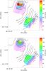 |
Fig. A.1
Integrated map of [C ii] obtained in the GREAT observations (contours) overlaid by colors of the [C ii] line intensity from the two PACS footprints. The top image shows the intensities in the original PACS footprints. In the bottom version this is resampled to the positions of the GREAT map with an effective resolution of the 17.2′′ beam. |
| Open with DEXTER | |
Appendix A.1: PACS spectroscopy
The [O i] and [C ii] lines were observed earlier in S 140 through the PACS instrument on board Herschel in the frame of a spectral scan at two individual pointings, one centered at IRS 1 and the other close to the cloud surface towards HD 211880. The PACS footprint is not fully sampled so that it may miss part of the flux between the pixels, but if we assume a source size of 5.5′′ or above that missing flux should be small so that we can use the data to check the consistency with the GREAT observations. The spectral resolution of PACS was insufficient to resolve the line, so that we can only compare integrated intensities.
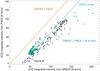 |
Fig. A.2
Measured intensities in the different pixels from Fig. A.1b as seen by GREAT and PACS. Green asterisks represent the footprint around IRS 1, black plus signs the footprint at the outer interface. The brown line shows the identity, the blue line represents an identity with an offset of 30 K km s-1. |
| Open with DEXTER | |
Figure A.1 compares our new intensity map with the PACS data for the two footprints. We see that the spatial structure of the emission peaks around IRS 2 and the interface is consistent between PACS and GREAT data. The PACS data just miss the global emission peak, but they peak at the position closest to the true maximum and they also trace the structure of the extended emission at the outer cloud interface. When comparing absolute intensities, however, we find systematically somewhat lower intensities in the PACS data than in the GREAT data.
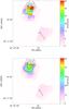 |
Fig. A.3
Integrated map of [O i] obtained in the GREAT observations (contours) overlaid on the colors of the [O i] line intensity from the two PACS footprints. The top image shows the intensities in the original PACS footprints with GREAT data convolved to 10′′ resolution. In the bottom version both maps are resampled to the positions of the GREAT map for the effective resolution of a circular 12′′ beam. |
| Open with DEXTER | |
To understand whether this is a calibration problem, we computed the pixel-to-pixel statistics in the resampled map. This is shown in Fig. A.2. We find a uniform behavior between both footprints; the PACS intensity is offset from the identity by about 30 K km s-1. This means that we do not have a calibration difference, but a difference in the absolute level. This can be naturally explained if there is a 30 K km s-1 contamination of the OFF position used as the reference in the PACS observations. The GREAT observations use a well-controlled OFF position 6.5′ southwest of the molecular cloud, while the chopped PACS observations involve a reference that falls 6′ into the molecular cloud. Some [C ii] emission from that region is quite likely and would explain the constant absolute offset between the GREAT and PACS intensities.
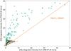 |
Fig. A.4
Measured intensities in the different pixels of Fig. A.3 as seen by GREAT and PACS. Green asterisks represent the footprint around IRS 1 and black plus signs the footprint at the outer interface when both data sets are resampled to a common 12′′ resolution (Fig. A.3b). Blue diamonds and orange triangles are obtained when we resample the GREAT data to the 25 pixels of the PACS array using the 9′′ PSF of PACS for the IRS 1 region and the interface, respectively (Fig. A.3a). The brown line shows the identity. |
| Open with DEXTER | |
As the [O i] emission is much less extended, we expect no OFF contamination in the PACS data for this line. Figure A.3 compares the spatial distribution of the [O i] integrated line emission measured by PACS with our GREAT observations. The spatial distributions of the emission seen through GREAT and PACS agree relatively well, having the peak again around IRS2, but for the individual intensities we find some significant deviations. Figure A.4 compares PACS and GREAT intensities from two different ways of resampling. One is shown in the lower panel of Fig. A.3, namely both maps are resampled to a common 4′′ grid with 12′′ resolution (green asterisk and black plus signs in Fig. A.4). Since the PACS map is not fully sampled, we extracted the flux based on the geometrical overlap. In the second method, we used the integrated intensity of the original 5 × 5 PACS spaxels, and resampled the GREAT data to each spaxel position (blue diamonds and orange triangles in Fig. A.3). The resulting trend is the same with both methods. There is a good match for the map around the interface and for the highest intensities close to IRS 2 at the northern boundary of the PACS field. However, across the PACS array centered at IRS 1, the intensities seem to be systematically too high. Off-contamination on the GREAT side can be excluded as it would show up as a constant offset like that seen in the [C ii] case. Moreover, we used the same reference position as for [C ii], and [O i] is rather less extended than [C ii] owing to the higher critical density. One can see in Fig. A.4 that the different ways of resampling the data do not make any significant difference. The PACS observer’s manual (v2.3) does not provide any direct
explanation. The wavelength of 63μm is not listed as a ghost from other strong emission lines and it is not in the leakage wavelength range. We can only speculate that this may be a stray-light problem where the strong [O i] emission just at the edge of the PACS footprint is partially picked up in the adjacent spaxels. Unfortunately, there are no calibration data available to verify that situation as the calibration observations were not set up to just miss the target. Hence, we cannot provide a quantitative explanation for the mismatch.
Appendix A.2: HIFI cut
|
Fig. A.5
[C ii] spectra taken with HIFI (black) and GREAT (red) along a 37 degree cut through IRS 1 and the cloud surface. The HIFI cut extends deeper into the cloud and only every second spectrum is plotted. The corresponding GREAT spectra were averaged in a 6′′ circle around the HIFI position. |
|
| Open with DEXTER | |
The [C ii] line was also observed by HIFI (Dedes et al. 2010) in a single strip going through IRS 1 and the surface, oriented to the same angle of 37 degrees east of north as our GREAT map. In Fig. A.5 we compare individual HIFI spectra along that cut at a half-sampled spacing with the corresponding GREAT spectra obtained by averaging all data in a 6′′ circle around the HIFI positions.
We generally find a very good match between HIFI and GREAT spectra, in particular the line shapes agree in all details, but at some positions the GREAT peak intensities are larger by a few percent up to 15%. First of all, this confirms the good relative calibration and pointing accuracy of both instruments/telescopes. The higher intensity of GREAT at an offset of −50′′ and + 12′′ could be due to the somewhat larger telescope beam of SOFIA leading to more intensity pickup from the surface at −50′′ and from the newly detected intensity peak north of IRS 1 at + 12′′.
Appendix B: The [O II] 145 μm/63 μm ratio
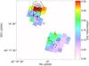 |
Fig. B.1
Observed ratio of the [O i] 145 μm to [O i] 63 μm line integrated intensity seen by PACS (colors) overlaid on the contours of the [O i] 63 μm emission measured by GREAT. |
| Open with DEXTER | |
In spite of the possible stray-light issue of the PACS [O i] map (see Appendix A.1), we can also try to use the [O i](145 μm)/ [O i](63 μm) line ratio to constrain the parameters of the PDRs in S 140, assuming that the ratio between both lines should be more robust than the simple integrated line intensity.
Because the excitation energy of the 145 μm line of 325 K lies above that of the 63 μm line (228 K) the [O i](145 μm)/ [O i](63 μm) measures temperature (or gas heating through the UV field) in the temperature range of about 300 K. In many cases, however, this ratio may be dominated by the optical depth in the 63 μm line (Kaufman et al. 1999; Malhotra et al. 2001). A low [O i](145 μm)/[O i](63 μm) compared to the PDR model
prediction is observed in many PDRs, and the foreground absorption, opacity effect of the [O i] 63 μm, and the cloud geometry are proposed as possible explanations (Liseau et al. 1999; Caux et al. 1999; Giannini et al. 2000; Okada et al. 2003). Liseau et al. (2006) provided the theoretical estimates of this ratio for different physical conditions. In the case of optically thin emission, a ratio above 0.1 can be achieved only when the gas temperature is >500 K and the collision partner is H2, which is unlikely. For the optically thick case, their calculation with the density of 3 × 104 cm-3 shows that the column density of N(H) >1024 cm-2 would be required to make the [O i](145 μm)/[O i](63 μm) ratio above 0.1.
Figure B.1 shows the integrated intensity ratio of [O i](145 μm)/[O i](63 μm) from the two PACS footprints centered at IRS 1 and at the interface observed in the frame of the Herschel key project WADI (Ossenkopf et al. 2011). For the interface parameters discussed above, the face-on PDR model produces a [O i](145 μm)/[O i](63 μm) ratio of 0.04, whereas the observed value is 0.17, i.e. about four times higher. If we interpret it through the inclination of the PDR in the same way as for the [C ii] line, the ratio asks for a geometrical amplification of the [O i] 145 μm line by a factor of four, two times lower than inferred from the [O i](63 μm)/[C ii] ratio in Sect. 4.5.
At IRS 2, [O i](145 μm)/[O i](63 μm) from the PACS observations is 0.3. For the PDR with a UV field of 5.6 × 10⁴χ0 and a density between 1.4 × 10⁵ and 106 cm-3 (Sect. 4.5), the predicted ratio is 0.03–0.045. Since the absorption by the cold gas at the back side of the PDR should affect only the 63μm transition, a factor of 7−10 of self-absorption is required to be consistent with the model predicted [O i](145 μm)/[O i](63 μm).
At IRS 1, the observed [O i](145 μm)/[O i](63 μm) is 0.1, which suggests PDR gas with a density of 103–104 cm-3 and a UV field of >106, but as discussed in Sect. 4.5, there is no consistent model for IRS 1.
© ESO, 2015
Current usage metrics show cumulative count of Article Views (full-text article views including HTML views, PDF and ePub downloads, according to the available data) and Abstracts Views on Vision4Press platform.
Data correspond to usage on the plateform after 2015. The current usage metrics is available 48-96 hours after online publication and is updated daily on week days.
Initial download of the metrics may take a while.