| Issue |
A&A
Volume 580, August 2015
|
|
|---|---|---|
| Article Number | A94 | |
| Number of page(s) | 21 | |
| Section | Extragalactic astronomy | |
| DOI | https://doi.org/10.1051/0004-6361/201424815 | |
| Published online | 07 August 2015 | |
Online material
Appendix A
Here we present the results for the frequency dependent light curve parameters including the entire range of shock parameters (see Table 1). The plots in this Appendix provide a global view of the changes in the slopes of the different stages in the (νm − Sm) plane and the light curve parameters.
A.1. Slopes of the energy loss stages
Figures A.1 and A.2 show the maps of the values obtained for the slopes of the different energy loss stages as a function of d, b, and s, indicating some colour levels (black, solid lines) in the plot to help identifying the values, and providing also a dashed line that separates the case of evolution towards a magnetically dominated from evolution towards particle dominated flows. This line is derived as follows: Taking into account that the magnetic energy density is uB ∝ B2 and using B ∝ R− b, we obtain uB ∝ R−2b. For particles, ue ∝ ∫n(γ)γdγ using n(γ) ∝ Kγ−s. Neglecting the evolution of γ with distance, we can assume ue ∝ K, and using K ∝ R−k and k = 2(s + 2)/3 if the jet expands adiabatically, we have uB/ue ∝ R−2b + 2(s + 2)/3. Imposing independence with distance brings the exponent to zero, which requires b = (s + 2)/3. If b< (s + 2)/3, the ratio grows with distance, whereas for b> (s + 2)/3 the ratio decreases with distance. Each panel shows the variation of ϵi (i = 1 Compton, i = 2 synchrotron, and i = 3 adiabatic) for 2 <s< 3 and 1 <b< 2 and a fixed value of d. The value of d is changing from top to bottom from d = −0.45 to d = 0.45 (see also the figure captions). The left column in both plots shows the maps of values of ϵC as a function of b and d. The vertical levels indicate that this slope is fairly independent of s for any values of b and d, and that it mainly changes with these two parameters. In the case of ϵS, the slope of the synchrotron stage, the situation is different, and s and d appear to be the most relevant parameters to determine it, although there is also a smooth gradient of this slope in the direction of b for the extreme values of d. Finally, the third column shows the maps of ϵA, which is most sensitive to d and b, and only shows a smooth variation with s.
A.2. Slopes of the frequency dependent light curve parameters
Figures A.3–A.6 show maps of the exponents of the frequency dependent light curve parameters as a function of s and b for different values of d. As mentioned earlier, the exponents for the flare amplitude and the flare time scale can be obtained either from the rising edge or the decaying edge of the light curve. In Figs. A.3 and A.4 we present these parameters obtained from the
rising edge and in Figs. A.5 and A.6 for the decaying edge of the light curves. In Figs. A.3 and A.4, each panel shows, from left to right, the variation in the flare amplitude exponent, ϵflare amp., the flare time scale exponent ϵflare time scale and the cross-band delay exponent, ϵdelay, for 2 <s< 3 and 1 <b< 2 and a fixed value of d. The value of d is changing from top to bottom from d = 0.45 to d = −0.45 (see also the figure captions). The amplitude of the flare undergoes a stronger variation with frequency for decreasing Doppler factors with distance (Fig. A.3) than for the increasing (Fig. A.4), as indicated by the colour-scales. In all cases, the slope grows with increasing s and b. The time lapse between the onset of the flare and the peak at each frequency is more sensitive to changes in frequency for decreasing Doppler factors with distance. This time lapse is more sensitive to b than to s, and the difference among frequencies becomes larger (smaller ϵflare time scale) for values of b closer to 1. Finally, the time lag between the peaks at different frequencies and a reference one has a similar behaviour with respect to the relevant parameters to the time lapse between onsets and peaks. The main difference is that there is not a large difference in the slopes between positive and negative values of d and that there are clear discontinuities in the values of the ϵtime lag for increasing Doppler factors, at certain values of s.
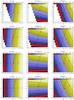 |
Fig. A.1
Parameter space plots for the variation of the slopes, ϵi as function of b and s while keeping the d parameter fixed. The columns show from left to right, the slope of the Compton stage, ϵC, the slope of the synchrotron stage, ϵS, and the slope of the adiabatic stage, ϵA. The exponent for the evolution of the Doppler factor, d, is from top to bottom d = −0.45, d = −0.30, d = −0.15, and d = 0. The black dashed line corresponds to a constant uB/ue ratio with distance (beq = (s + 2)/3)), i.e. to the left of this line the jet flow tends to be magnetically dominated with distance and to the right the jet tends to be particle energy dominated with distance. |
| Open with DEXTER | |
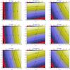 |
Fig. A.2
Same as Fig .A.1 for d = 0.15, d = 0.30, and d = 0.45. |
| Open with DEXTER | |
In Figs. A.5 and A.6 we show the variation of the exponent for the flare amplitude and the flare time scale obtained from the decaying edge of the light curve. The exponent for the flare amplitude ϵflare amp. decay decreases with d. For d< 0 the absolute value of the exponent increases with s and b. However, for d> 0 the distribution of ϵflare amp. decay changes: The exponents still increase with s but larger values are obtained towards b = 1. The exponent for the flare time scale derived from the decaying edge of the light curve, ϵflare time decay is small, typically <0.05. The value and its distribution depend strongly on d. For d< 0 the distribution is smooth and the values decrease with s and b. Nearly no variation in ϵflare time. decay is obtained for d> 0 (see second column in Figs. A.5 and A.6).
Figures A.7 and A.8 show the expected time lags (in years) between the peaks at 5 GHz, 15 GHz, and 140 GHz and our reference frequency, 345 GHz (left, central and right columns, respectively), for different values of d (different rows), as a function of s and b. The cross-band delays become shorter for increasing Doppler factor with distance as indicated by the colour scales at the top of the panels. The time lags between the reference frequency and low frequencies are typically more sensitive to b increasing as this parameter tends to 1, whereas the time lags between 140 GHz and 345 GHz show significant values only for decreasing Doppler factor with distance and higher sensitivity to the spectral slope s.
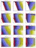 |
Fig. A.3
Parameter space plots for the variation of frequency dependent single-dish light curve parameters obtained from the rising edge of the light curves as function of b and s while keeping the d parameter fixed. The columns show from left to right the exponent for the variability amplitude, ϵflare amp., the exponent for the variability time scale, ϵflare time scale, and the exponent for the time lag, ϵdelay. The exponent for the evolution of the Doppler factor, d, is from top to bottom d = −0.45, d = −0.30, d = −0.15, and d = 0. The black dashed line corresponds to a constant uB/ue ratio with distance (beq = (s + 2)/3)), i.e. to the left of this line the jet flow tends to be magnetically dominated with distance and to the right the jet tends to be particle energy dominated with distance. |
| Open with DEXTER | |
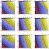 |
Fig. A.4
Same as Fig. A.3 for d = 0.15, d = 0.30, and d = 0.45. |
| Open with DEXTER | |
|
Fig. A.5
Parameter space plots for the variation of frequency dependent single-dish light curve parameters obtained from the decaying edge of the light curves as function of b and s while keeping the d parameter fixed. The columns show from left to right, the exponent for the variability amplitude, ϵvar. amp., the exponent for the variability time scale, ϵvar. time scale, and the exponent for the cross-band delay, ϵdelay. The exponent for the evolution of the Doppler factor, d, is from top to bottom d = −0.45, d = −0.30, d = −0.15, and d = 0. The black dashed line corresponds to a constant uB/ue ratio with distance (beq = (s + 2)/3)), i.e. to the left of this line the jet flow tends to be magnetically dominated with distance and to the right the jet tends to be particle energy dominated with distance. |
|
| Open with DEXTER | |
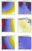 |
Fig. A.6
Same as Fig. A.3 for d = 0.15, d = 0.30, and d = 0.45. |
| Open with DEXTER | |
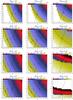 |
Fig. A.7
Parameter space plots for the for the time lag between three selected frequencies as function of b and s while keeping the d parameter fixed. The columns show from left to right, the (345−5) GHz time lag, the (345−15) GHz time lag, and the (345−86) GHz time lag. The exponent for the evolution of the Doppler factor, d, is from top to bottom d = −0.45, d = −0.30, d = −0.15, and d = 0. The black dashed line corresponds to a constant uB/ue ratio with distance (beq = (s + 2)/3)), i.e. to the left of this line the jet flow tends to be magnetically dominated with distance and to the right the jet tends to be particle energy dominated with distance. |
| Open with DEXTER | |
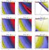 |
Fig. A.8
Same as Fig. A.7 for d = 0.15, d = 0.30, and d = 0.45. |
| Open with DEXTER | |
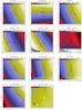 |
Fig. A.9
Modified Compton stage model using d = 0. The top row shows the slopes for the different energy loss stages from left to right: compton, synchrotron, and adiabatic stage. The delay between selected frequencies with respect to 345 GHz in years is plotted in the second row from left to right: delay to 5 GHz, delay to 15 GHz and delay to 86 GHz. The third row presents the frequency dependent light curve parameters obtained from the rising edge of the light curve from left to right: flare amplitude, flare time scale and cross frequency delay. The bottom row shows the exponent for the flare amplitude and the flare time scale as derived from the decaying edge of the light curve. The black dashed line corresponds to a constant uB/ue ratio with distance (beq = (s + 2)/3)), i.e. to the left of this line the jet flow tends to be magnetically dominated with distance and to the right the jet tends to be particle energy dominated with distance. |
| Open with DEXTER | |
© ESO, 2015
Current usage metrics show cumulative count of Article Views (full-text article views including HTML views, PDF and ePub downloads, according to the available data) and Abstracts Views on Vision4Press platform.
Data correspond to usage on the plateform after 2015. The current usage metrics is available 48-96 hours after online publication and is updated daily on week days.
Initial download of the metrics may take a while.