| Issue |
A&A
Volume 556, August 2013
|
|
|---|---|---|
| Article Number | A76 | |
| Number of page(s) | 23 | |
| Section | Interstellar and circumstellar matter | |
| DOI | https://doi.org/10.1051/0004-6361/201220717 | |
| Published online | 31 July 2013 | |
Online material
Appendix A: Newly discovered outflows
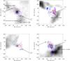 |
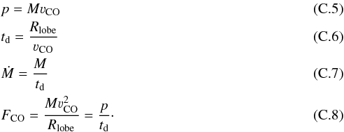
Fig. A.1
Regions around the new outflow structures (Us), showing the SCUBA 850 μm emission in the background, the contour map of the integrated line wings, the sources from the sample in this study marked with pluses and the Us indicated with arrows. The nearby submillimeter cores are marked with circles and infrared sources with a cross. (Top left) The region around IRS 63. (Top right) The region around IRS 37. (Bottom left) The region around WL 12. (Bottom right) The region around IRS 44. |
| Open with DEXTER | |
From detailed spectral analysis, new bipolar outflow structures were discovered in several CO maps, not belonging to any of the sources in the embedded source sample of van Kempen et al. (2009c). In this section we look for other suitable candidates of embedded sources. The partial coverage of these outflows extends the field in which to look for a candidate.
-
The outflow structure U1 southwest of IRS 63 mayoriginate from the submillimeter core SMM J 163133–24032,which was matched by Jørgensenet al. (2008) with the Spitzer YSOcandidate SSTc2d J163134.29-240325.2 (Evanset al. 2009), located24″ away, classified as a Class I source with Lbol = 0.88 L⊙ and Tbol = 870 K.
-
For U2, selecting a candidate is somewhat difficult, as only a small piece of the red lobe is covered and therefore the direction of the originating source is unknown. The most likely candidate is the submillimeter core SMM J 163143–24003 (Jørgensen et al. 2008) at 2.2′ northeast of IRS 63 (see Fig. A.1) with a dust temperature of 15 K. No infrared source is known near this location.
-
U3 is located to the west of IRS 37. The elongated structure and direction of the outflow suggest that the powering source is located to the southwest. The large submillimeter core SMM J162713–24295 (Jørgensen et al. 2008) is a likely candidate (see Fig. A.1) with a dust temperature of 18 K. The shape of this submillimeter core is consistent with the outflow direction, which is usually perpendicular to the ridge (Anathpindika & Whitworth 2008). Again, no infrared source is known at this location.
-
The outflow U4 is clearly visible in the WL 12 map (Fig. A.1). The center of origin is about 16:26:40, − 24:35:27. There are no submillimeter cores or infrared sources nearby. Estimates of a SED or Tbol are therefore not possible at this time.
-
U5 is located to the west of IRS 44 (Fig. A.1). Towards the southwest is submillimeter core J162721.7-244002, (Di Francesco et al. 2008), which is a possible candidate for the powering source. However, just like U3, there is no infrared source at this position. No temperature was derived for this core, but the 450 and 850 μm fluxes in combination with the nondetection at 70 μm and shorter wavelengths indicate a very low dust temperature between 5 and 10 K.
-
Only the blue lobe of U6 is detected, but there are no submillimeter cores or infrared sources nearby. Estimates of a SED or Tbol are therefore not possible at this time.
The Us are clearly peculiar objects. Only U1 could be assigned to a YSO candidate, a submillimeter core with an infrared detection. U2, U3 and U5 are interesting since they have a possible source of origin in submillimeter cores without infrared detection, suggesting either a very low temperature and luminosity, a very deeply embedded object, an edge on geometry or a new kind of object, producing an outflow or some other mechanism producing swept-up gas. For U4 and U6 not even a submillimeter core was detected. U2, U5 and U6 are only marginally covered and therefore possibly no new outflows: they may be part of the main outflow in the map and only seem separate due to density variations in the envelope. However, for U1, U3 and U4 this is not very likely considering their morphology. Full spatial coverage of low-J CO lines of these regions may provide an answer. Far-infrared fluxes provided by Herschel may help to define the cold cores (Bontemps et al. 2010, e.g.) and derive their properties, to conclude whether they can be the powering sources of these outflows.
Appendix B: Comparison with other outflow studies
Of our sample of 16 sources, 11 sources were studied previously (Bontemps et al. 1996; Sekimoto et al. 1997; Kamazaki et al. 2003; Bussmann et al. 2007; Nakamura et al. 2011) but often with different derived properties. We compare the results, methods and available observations in Tables B.1 and B.2.
The sources studied by Bontemps et al. (1996) have a systematic offset in FCO due to their opacity correction of 3.5. If this factor is removed, their outflow forces are still typically a factor of 2 higher if we use the same annulus method (M6) on our data set (see Fig. 5). Since their rms level is similar to our study and other effects due to coverage or method can be excluded, the only other explanation may be the determination of the inner velocity limit: Bontemps et al. used Tpeak/10 for νin, but Tpeak is source dependent and easily affected by the presence of foreground clouds. When the inner velocity limit is moved 1 km s-1 inwards, the outflow force is increased by a factor of 2 (see Fig. D.1). The inclination factor of 2.9 for a constant i = 57° does not cause significant underestimates, since none of these five sources have an inclination of 70° which generally requires a larger correction factor (see Fig. 5).
The values found by Sekimoto et al. (1997) agree very well (within a factor of 1.8) with the results in this study, as expected considering their methods and data quality. However, they derived an opacity in the line wings from 13CO lines of 3.0 for the 2–1 lines, similar to CB92. The results for LFAM 26 and Elias 29 in the study from Bussmann et al. (2007) are both a factor of ~5 higher. Inspection of the individual parameters shows that this difference is dominated by the effect of integrated mass, which is more than 10 times larger in their study, whereas their dynamical time is only twice as long compared to our results. The observations presented by Bussmann et al. cover the entire outflow of Elias 29 and LFAM 26. Apparently the mass is not uniformly spread over the outflow lobes, so the outflow momentum may not be conserved along the lobe in this case.
The outflow force for Elias 33 also agrees well with the value found by Kamazaki et al. (2003), considering their opacity correction of 5.4. Considering their high rms level and 3σ cut-off, their derived outflow velocities are only 5.6 and 3.6 km s-1, for the blue and red lobe, respectively, versus 12.0 and 10.0 km s-1 in this study. This would decrease the outflow force with a factor of 4–5, but this is compensated by the total (uncorrected) mass derived by Kamazaki et al. which is more than 5 times larger than derived in this study.
Comparison of the outflow force between this study and other outflow studies.
Comparison of the methods and observation properties between this study and other outflow studies.
Our results do not match well with the results from Nakamura et al. (2011): LFAM 26 is comparable, but our value for Elias 29 is 7 times lower while the value for Elias 32/33 is 2 times higher. The reason for this discrepancy may be the choice of inclination angles: the adopted value of 80° for Elias 29 and LFAM 26 with the projection formula sini/cosi used by Nakamura results in a correction factor of 6, the adopted value of 57° for Elias 32/33 gives a correction of 1.6, while in this study an inclination of 50° was assumed for Elias 29 (correction factor 0.45) and i = 70° for Elias 32/33 (correction factor 1.6). The 3σ cutoff and low S/N data used by Nakamura et al. would have resulted in lower values of the outflow force for all three sources with a factor 2–4, but this is counterbalanced by the use of larger correction factors (6 versus 1.1 and 1.6 versus 0.45).
This section shows again that, in order to compare and combine outflow studies, similar methods have to be applied, since results from the studies discussed can differ by more than one order of magnitude. Since opacity and inclination cause the largest variations in the outflow force, it is essential to derive these properties as accurately as possible.
Appendix C: Mass derivation
The main physical parameters of the outflow are the mass, M, the velocity, νCO (defined as | νout − νsource |), and the projected size of the lobe Rlobe, for both the blue and red lobe. The mass is calculated from the column density assuming an excitation temperature of 100 K (e.g. Yıldız et al. 2012). The column density of the 12CO upper level u (in this case J = 3) is derived from the integrated intensity of the line wings as follows. 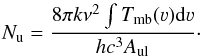 (C.1)The column density of the upper level, Nu (cm-2), is converted to H2 column density N by
 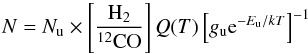 (C.2)with Q(T) the partition function and using H2/12CO = 1.2 × 10⁴ (Frerking et al. 1982) and N is converted to mass in grams using
 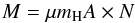 (C.3)with a mean molecular weight μ of 2.8 used to include He (Kauffmann et al. 2008) and A the physical area covered by one pixel. Summarizing, the conversion from integrated intensity to mass is a multiplication with constant K:
 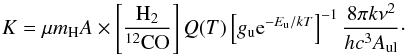 (C.4)With these basic physical quantities, a number of outflow parameters can be derived: the momentum, p, the dynamical age, td, the mass outflow rate, Ṁ and the outflow force, FCO. The basic equations are:
The velocity, νCO, often called νmax, is not a well-constrained parameter: due to the inclination and the shape of the outflow, often following a bow shock including forward and transverse motion, the measured velocities along the line of sight are not necessarily representative of the real velocities driving the outflow (Cabrit & Bertout 1992). This is the main reason why various methods have been developed to derive the outflow force, where a correction factor is often applied to compensate for these effects.
Appendix D: Influence of assumptions and data quality
Apart from the analysis method, a number of choices, observational properties and assumptions may influence the value of the outflow force. The effects are tested using the νmax method (M1) on a small sample of four targets: Elias 29, IRS 54, HH 46 and IRAS4A. The results are presented in Fig. D.1. In each plot, the resulting outflow force is normalized to the “standard” value, which is the outflow force resulting from the best estimate of that parameter using the recipe in Sect. 4.2.
Appendix D.0.1: Inner velocity limits
The inner velocity limits are determined from the width of the (averaged) off-source spectra. In general, it can be difficult to determine where the outflow emission blends in with the ambient envelope emission (see also Sect. 4.3). The first panel shows how the outflow force changes if the inner velocity limits are shifted simultaneously inwards (negative) or outwards (positive), relative to the best guess based on off-source emission. When the inner limits are moved inwards, more and more integrated emission is taken into account, also including more envelope emission, increasing the mass of the outflow up to a factor of 5, but certainly within 0.5 km s-1 the significance remains within a factor of 2. Moving the limits outwards decreases the outflow force by a factor of 2. For IRAS4A, the outflow force increases only slightly moving inwards: due to the high velocities involved, the integrated mass is not the dominant parameter. For the intensity-weighted methods the change of the inner velocity limit changes the outflow force even less since the intensity at low velocities does not contribute much to the total outflow force.
Appendix D.0.2: Spatial coverage
Bontemps et al. (1996) suggested that it does not matter how much of the outflow emission is spatially covered for calculating the outflow force, as long as the correct size Rlobe is taken for the spatially covered spectra, because the momentum is conserved along the outflow lobes. To test this assumption, a range of radii were chosen starting at the central position in each map and finishing at the border of the map. When taking a larger radius, more and more spectra are integrated, but Rlobe simultaneously increases. Nearby outflows from other sources are excluded beforehand. Panel 2 in Fig. D.1 shows that the outflow force indeed remains constant as a function of radius. The outflow force of IRAS4A increases significantly up to a factor 3 due to the inclusion of a “bullet” and high-velocity emission starting around 90″. Elias 29 decreases slightly at larger radii, due to the two broken receivers as shown in Fig. 3, where parts of the lobes are missing. This figure proves that the outflow force can be analyzed with partial coverage as long as it is centered on the source position, but one has to be careful with emission from other sources, “bullet” emission and when regions of data are missing.
 |
Fig. D.1
Influence of observational properties and choices on the resulting value of the outflow force, using M1 (νmax) on Elias 29, IRS 54, HH 46 and IRAS4A, which all have clear, isolated outflows. See text for description of each category. It follows that these observational properties and choices in the analysis procedure affect the outflow force up to a factor of 4–5. |
| Open with DEXTER | |
Appendix D.0.3: Spectral binning
Astronomical spectra are often rebinned to lower spectral resolution in order to decrease the rms, since lines of outflows have broad spectral profiles. When the outflow velocity limits are based on the rms level, binning to larger bin sizes may influence the outflow force significantly. This is investigated in panel 3 in Fig. D.1. The outflow force remains constant within a factor of 2 for Elias 29, IRS 54 and IRAS4A. Inspection of the mass as function of bin size (not shown here) shows a decrease of the integrated mass, but this is apparently compensated by the higher outer velocities. On the other hand, HH 46 shows a significant increase of outflow force. This is due to the low S/N of this data set: the lower rms moves νmax rapidly outwards while the inner velocity remains almost constant. Therefore, one has to be careful with binning spectra when using an rms cut-off for the velocities, since the choice of binning may further increase the outflow force significantly. The intensity-weighted methods, such as M7, are less affected by rebinning.
Appendix D.0.4: Cut-off level
The rms level determines the outer velocity and therefore the outflow force depends on the quality of the data. In order to investigate this, the observed high quality spectra are convolved with an artificial noise signal and the velocity limits are redetermined with the new rms. The resulting outflow force as function of new rms is shown in panel 4 of Fig. D.1: the outflow force can be underestimated by a factor of 5–10 for large noise levels (S/N < 5 for the wing emission). The outflow force of HH 46, which already has a large noise level to start with, is likely to be underestimated.
In some studies, the rms cut-off is not taken at 1σ, but rather 3σ or even 10σ to determine the outer velocities. The effect of taking a cut-off at multiple σ is investigated in panel 5. The outflow force decreases slowly when taking a stricter cut-off but the overall effect remains within a factor of 3–4, except for the spectra of HH 46 with low S/N.
Appendix D.0.5: vout: ratio cut-off
Due to the disadvantages of using an rms cut-off described above, another method is sometimes applied. The cut-off limit is defined as e.g. 1% of the intensity at the inner velocity limit of the outflow wing (DC07). In that case, the cut-off level depends on the brightness of the source itself, rather than the quality of the observations. The difference between these two methods is investigated in Panel 6 of Fig. D.1, where the outflow force is normalized to the value found by the rms cut-off. The outflow force is likely to be underestimated for a ratio lower than 50. For the higher ratios, the outflow force remains constant, which
means that the outflow wing is sufficiently steep: the outer velocity is not affected by this small change in the cut-off level.
Appendix D.0.6: Summary
Observational properties and choices in the analysis procedure can affect the outflow force up to a factor of 4–5. Small changes in the inner velocity limit, the rms level, the cut-off significance and binning do not change the outflow force more than a factor of 2. It is demonstrated that the spatial coverage in principle does not influence the outflow force, indicating that this is a conserved quantity. Also, choosing a percentage of the emission at the inner velocity limit for the cut-off does not in principle change the outflow force, as long as the percentage is low enough. The most important factor to consider is the S/N, as shown in the results of HH 46 with a higher noise level. A strong dependence of the outflow force on the noise level (Fig. D.1) implies that the methods described cannot always be applied directly. When combining the results from different studies, using different methods, assumptions and/or data quality, scatter up to a factor of 5 can be expected.
Appendix E: Outflow parameters from other studies
Outflow and evolutionary parameters from other studies used in evolutionary trends.
Appendix F: Spectra overview
 |
Fig. F.1
Overview of relevant outflow spectra. Each diagram shows from top to bottom the strongest red wing spectrum, the strongest blue wing spectrum and an off-source spectrum. νsource (dashed line) and the integration limits (dotted lines) are indicated. A dash-dotted line indicates the baseline. Positions of each spectrum are indicated in parentheses. |
| Open with DEXTER | |
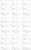 |
Fig. F.1
continued. |
| Open with DEXTER | |
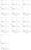 |
Fig. F.1
continued. |
| Open with DEXTER | |
Integration limits of the 12CO J = 3–2 line wings.
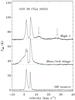 |
Fig. F.2
Spectrum with extremely high-velocity (EHV) emission in the GSS 30 map as indicated by arrows, originating from the Class 0 source VLA 1623. Any outflow emission from GSS 30 itself can not be disentangled from VLA 1623 in the present observations. From top to bottom: one high-velocity position (−45″, 0″), one wing position (−30″, −22 |
| Open with DEXTER | |

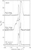 |
Fig. F.3
Outflow spectra of Elias 32/33, showing a red wing spectrum (top), blue wing spectrum (middle) and off-source spectrum (bottom). νsource (dashed line) and the integration limits (dotted lines) are indicated. A dash-dotted line indicates the baseline. Positions of each spectrum are indicated in brackets. Especially the blue wing shows a double structure, suggesting blending of outflow emission of two separate sources. |
| Open with DEXTER | |
© ESO, 2013
Current usage metrics show cumulative count of Article Views (full-text article views including HTML views, PDF and ePub downloads, according to the available data) and Abstracts Views on Vision4Press platform.
Data correspond to usage on the plateform after 2015. The current usage metrics is available 48-96 hours after online publication and is updated daily on week days.
Initial download of the metrics may take a while.