| Issue |
A&A
Volume 554, June 2013
|
|
|---|---|---|
| Article Number | A14 | |
| Number of page(s) | 24 | |
| Section | Extragalactic astronomy | |
| DOI | https://doi.org/10.1051/0004-6361/201220768 | |
| Published online | 30 May 2013 | |
Online material
Appendix A: The combination of FUV and dust emission as a proxy to the attenuation
While we have shown in Sect. 3.1.2 that the determination of the FUV attenuation with CIGALE is reliable, we examine here whether and how the results we have obtained are affected by using an alternative method for computing the attenuation and therefore the face-on optical depth. Several relations exist in the literature to quantify the attenuation from the FUV and the emission of the dust. These relations have generally been derived from the observation of unresolved star-forming galaxies (Cortese et al. 2008; Buat et al. 2011b; Hao et al. 2011). Boquien et al. (2012) have also derived a similar relation but on subregions in star-forming galaxies using CIGALE. Even though it yields attenuations close to that of previous relations, we do not consider it here as it has also been determined using CIGALE. Among the relations from the literature, Boquien et al. (2012) found that the one provided by Hao et al. (2011) yields the largest difference with the attenuation determined with CIGALE in resolved galaxies: ⟨ΔAFUV⟩ = 0.156 ± 0.056 mag. We therefore adopt this relation, as it will be indicative of the maximum deviation that could be induced by such an attenuation tracer compared to SED modelling. In Fig. A.1, we present the relations between the gas surface density and the FUV face-on optical depth determined from the formula published in Hao et al. (2011), assuming a slab geometry.
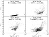 |
Fig. A.1
Face-on optical depth in the FUV band determined from the FUV and dust emission (Hao et al. 2011) versus the atomic total gas mass surface density in units of M⊙ pc-2. |
| Open with DEXTER | |
We see that using an alternative method for determining the attenuation leaves the relations qualitatively unchanged. After verification, the relations provided by Cortese et al. (2008) and Buat et al. (2011b) show little qualitative difference from the relation of Hao et al. (2011). However, the lower attenuations yielded by the relation of Hao et al. (2011) naturally affect the quantitative relations between the face-on optical depth and the gas surface density  (A.1)and
  (A.2)These relations yield smaller optical depths. Averaging over the entire sample, we obtain ⟨ΔτFUV/τFUV⟩ = 0.02 ± 0.04 when taking only the gas surface density into account, and ⟨ΔτFUV/τFUV⟩ = 0.10 ± 0.07 when taking into account both the gas surface density and the metallicity. The amplitude of these shifts is not larger than the error bars on the optical depths deduced from the uncertainties on the FUV attenuation provided by CIGALE. Therefore the use of different methods for determining the attenuation should only have a limited impact on the derived optical depth, with offsets of the order of 10%.
Appendix B: Dust emission as a proxy to the gas surface density
If the 21 cm emission is a direct tracer of the atomic gas, as mentioned earlier, the molecular gas is generally traced indirectly through CO emission. An alternative way to measure the total gas content in a galaxy is through the emission of the dust. As gas and dust are intimately intertwined, assuming a given gas-to-dust mass ratio one can retrieve the gas mass from the dust mass. Both methods have different biases. Whether the gas mass determination method affects our results or not is important to estimate their reliability.
One common method for determining the dust mass is to fit the FIR emission with a modified black body (e.g. Boselli et al. 2002; James et al. 2002; Eales et al. 2010, 2012,and many others). It is described in Eq. (B.1)  (B.1)with fν the flux density, D the distance of the object, h the Planck constant, ν the frequency, c the speed of light in vacuum, k the Boltzmann constant, T the temperature of the dust, κ the dust emissivity taken at frequency νκ, β the emissivity index, and Mdust the dust mass. Following Draine (2003a) we adopt κ = 0.192 m2 kg-1 at νκ = 857 GHz (350 μm). The value of β is the subject of an intense debate in the literature. A value between 1.5 and 2.0 is adequate for star-forming galaxies. Even though β can vary from region to region (Smith et al. 2012), Boselli et al. (2012) found that β = 1.5 best reproduces the FIR properties of the star-forming galaxies in the HRS sample. We therefore adopt their value. Note, however, that this emissivity has been determined from a dust model that assumes β = 2 rather than β = 1.5, which may induce a bias in the dust mass. We determine the dust mass by fitting Eq. (B.1) to the data at 70 μm, 250 μm, and 350 μm, using the curve_fit function in the scipy library (Jones et al. 2001), which is based on a Levenberg-Marquardt algorithm. This combination of bands allows us to get a good handle on the dust temperature because these bands straddle the FIR emission peak, and the dust mass as the 350 μm band does not show a strong dependence upon temperature variations. In the case of NGC 2403, the 70 μm emission comes from a distinctly different dust component rather than the dust emitting at longer wavelength. As a consequence, the dust mass within this galaxy will be underestimated. In Fig. B.1, we compare the gas mass estimated from the dust mass, versus the one derived from HI and CO emission. In both cases we use the metallicity-dependent conversion factors of Boselli et al. (2002) which assumes a gas-to-dust mass ratio of 160 for 12 + log O/H = 8.91.
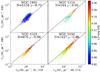 |
Fig. B.1
Total gas surface density derived from a modified black-body fit (Eq. (B.1)) of the FIR data from 70 μm to 350 μm versus the total gas surface density derived from the combination of HI and CO observations. The colour of each dot indicates the metallicity indicated by the scale on the right. The black lines show the 1-to-1 relation between these quantities. |
| Open with DEXTER | |
We see that there is a tight correlation between the total gas surface density derived with a modified black body and from the combination of HI and CO observation as shown by the high value of the Spearman correlation coefficient for NGC 2403 (ρ = 0.79), NGC 4254 (ρ = 0.95), NGC 4321 (ρ = 0.96), and NGC 5194 (ρ = 0.95). We observe that the surface densities obtained using either method are similar even though there are some small offsets, generally towards lower masses except for NGC 2403. However, they are small compared to the full dynamical range.
To verify whether determining the total gas surface density affects the results, we plot in Fig. B.2 the relation between the face-on optical depth and the total gas surface density derived from a modified black body fit.
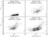 |
Fig. B.2
Face-on optical depth in the FUV band versus total gas surface density determined by fitting the FIR emission with a modified black body as described in Eq. (B.1). |
| Open with DEXTER | |
When comparing this to Fig. 7, we see that the results are very similar. The Spearman correlation coefficients for NGC 4254, NGC 4321, and NGC 5194 yield values close to what is found when combining CO and HI observations. However, in the case of NGC 2403 there is a significant decrease from ρ = 0.72 to ρ = 0.45. This could be due to the lower metallicity of this galaxy (⟨12 + log O/H⟩ = 8.90) compared to the rest of the sample (⟨12 + log O/H⟩ = 9.20). As such there could be a significant quantity of dark molecular gas not traced by CO. Quantitatively, the relations we derive are close to Eqs. (12) and (13)  (B.2)and
 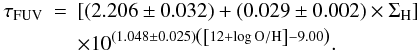 (B.3)These relations yield similar optical depths. Averaging over the entire sample, we obtain ⟨ΔτFUV/τFUV⟩ = 0.09 ± 0.05 when taking only the gas surface density into account, and ⟨ΔτFUV/τFUV⟩ = − 0.02 ± 0.06 when taking into account both the gas surface density and the metallicity. The amplitude of these shifts is not larger than the error bars on the optical depths deduced from the uncertainties on the FUV attenuation provided by CIGALE. Therefore the use of different methods for determining the gas surface density should only have a limited impact on the derived face-on optical depth, with offsets of the order of 10%.
Appendix C: Computation of the HI surface density
In Sect. 3.2 we provide a relation to compute the HI mass surface density. It is derived in the following way. First we consider this well-known relation linking NHI, the HI column density in atoms cm-2, to the brightness temperature TB in K 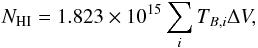 (C.1)with ΔV in m s-1. Considering that 1 M⊙ pc-2 = 1.248 × 10²⁰ atoms cm-2, we have
 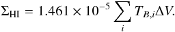 (C.2)The brightness temperature and the flux density per beam are related through the following equation
  (C.3)with P the angular power pattern of the beam, dΩ the solid angle, and mb denoting the main beam. For a Gaussian beam with a full width half maximum size Δα and Δδ along the major and minor axes, it easily comes that
  (C.4)Combining the two previous equations we get
  (C.5)Inserting this relation into Eq. (C.2)
  (C.6)Assuming that Δα and Δδ are expressed in arcsec, Si in Jy per beam, and ΔV in m s-1, a simple numerical application yields
 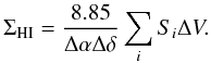 (C.7)
(C.7)
Appendix D: Impact of different CO transitions
As explained earlier, to trace the molecular gas this study relies on the CO(2 − 1) transition. Yet different transitions may yield different results. The intensity of the emission of the various CO transitions depends not only on the abundance of CO but also on the local physical conditions of the molecular gas, such as the density or the temperature. For a given quantity of CO, a high-level transition will trace more closely the denser and warmer part of the gas. Disentangling between these effects is particularly challenging and would require a dedicated study of the sample with appropriate data. Here, we do not attempt to separate these parameters; instead, we examine whether and how using different transitions would affect our results.
To complement our CO(2 − 1) data, we need additional transitions at a resolution that is similar or better than 30′′. This is a particularly limiting factor because CO(1 − 0) observations have a resolution twice as coarse as that of CO(2 − 1) for a given instrument. For higher order transitions, such as CO(3 − 2), observations are difficult to carry out as they require optimal atmospheric conditions. Nevertheless, 3 galaxies in our sample have adequate CO(3 − 2) maps to further our study. As part of the JCMT Nearby Galaxies Legacy Survey (Wilson et al. 2009), Bendo et al. (2010) published a CO(3 − 2) map of NGC 2403, and Wilson et al. (2009) maps of NGC 4254 and NGC 4321. For NGC 5194, Koda et al. (2011) have published a high-resolution single-dish CO(1 − 0) map which we adopt. Additional CO(1 − 0) observations of several galaxies in the sample have been published by Kuno et al. (2007). Unfortunately, their 15′′ beam is not Nyquist-sampled which makes the maps unsuitable for a pixel-by-pixel analysis. In Fig. D.1 we present the molecular gas surface density derived from the baseline CO(2 − 1) observations and the CO(3 − 2) ones (CO(1 − 0) for NGC 5194). Note that we divided our CO(2 − 1) intensities by a factor of 0.89 to scale them to the CO(1 − 0) line. We also scaled the CO(3 − 2) observations to CO(1 − 0) by dividing the intensities by a factor of 0.34 (Wilson et al. 2009).
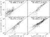 |
Fig. D.1
Molecular gas surface densities computed from CO(3 − 2) observations (CO(1 − 0) for NGC 5194) versus the molecular gas surface densities computed from the CO(2 − 1) transition. All CO lines have been scaled to the CO(1 − 0) line in order to apply the same XCO factor. The black line represents the 1-to-1 relation where both lines yield the same molecular gas surface densities. |
| Open with DEXTER | |
Visibly there is a strong correlation between CO(2 − 1) and other CO lines, with the Spearman correlation coefficient ranging from ρ = 0.68 for NGC 2403 to ρ = 0.96 for NGC 5194. In Fig. D.2 we plot the relation between the face-on optical depth and the gas mass surface density.
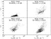 |
Fig. D.2
Same as for Fig. 3 with the molecular gas surface density determined from the CO(3 − 2) line (CO(1 − 0) for NGC 5194). |
| Open with DEXTER | |
We see that qualitatively the use of different CO transitions does not affect the global trends between these quantities and that the qualitative relations remain unchanged. We note, however, that there are far fewer datapoints for NGC 5194, which makes the flattening at low surface densities less evident. After inspection of the images, these are regions on the outskirts of the galaxy which are not in the field-of-view of the CO(1 − 0) map and have therefore been eliminated from the analysis. We should note that as commented by Wilson et al. (2009) and Bendo et al. (2010), there is a significant scatter in the ratio between the CO(3 − 2) line and lower CO transitions. It has been suggested that the CO(3 − 2) line is more closely associated with molecular gas fueling star formation than lower order lines, which may contribute to the pixel-to-pixel scatter.
Quantitatively, the relations we derive are close to Eqs. (12) and (13)  (D.1)and
 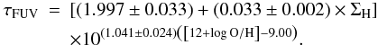 (D.2)These relations yield similar optical depths. Averaging over the entire sample, we obtain ⟨ΔτFUV/τFUV⟩ = 0.08 ± 0.05 when taking only the gas surface density into account, and ⟨ΔτFUV/τFUV⟩ = 0.05 ± 0.04 when taking into account both the gas surface density and the metallicity. The amplitude of these shifts is not larger than the error bars on the optical depths deduced from the uncertainties on the FUV attenuation provided by CIGALE. Therefore, the use of different CO transitions to determine the gas surface density should only have a limited impact on the derived face-on optical depth, with offsets of the order of 10%.
Appendix E: Relation with the molecular fraction
Whether the attenuation chiefly takes place in HI or H2 dominated regions gives us an interesting insight into radiation transfer in galaxies. In Fig. E.1 we show the FUV attenuation versus the molecular fraction.
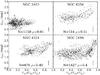 |
Fig. E.1
Relation between the molecular gas fraction and the attenuation. There is a clear trend, with increasing molecular fraction the attenuation increases, with the exception of NGC 2403 which shows no trend. This is consistent with the trends observed in Fig. 3. The number of elements and the Spearman correlation coefficient are indicated at the bottom of each panel whereas the uncertainty on AFUV is shown in the bottom-right corner. |
| Open with DEXTER | |
The regions that have a low molecular fraction generally correspond to peripheral regions. In the case of NGC 2403 we do not see any trend of the attenuation with the molecular fraction. Conversely the other three galaxies show two regimes. Up to a molecular fraction of 0.6 − 0.8, there is little to no trend, the attenuation remaining constant. Beyond this limit, the attenuation strongly increases with the molecular fraction. This suggests that where the molecular fraction is high, the attenuation is strongly linked to the quantity of molecular gas. At lower molecular fraction it is possible that the atomic gas plays a larger role in the attenuation. However, there could also be mixing effects if the FUV attenuation is driven by regions more closely linked to molecular gas even in low-density regions. We examine this possibility in more detail in Sect. 5.2.
Appendix F: Impact of the geometry
F.1. Attenuation-optical depth relations
For this study, we have adopted a slab geometry. However, as mentioned in Sect. 5.1, other geometries can also be considered. First of all, we examine the case of a sandwich model. Following Boselli et al. (2003), the relation between the face-on optical depth τλ and the attenuation is 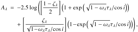 (F.1)with ζ the height ratio between the dust and stars layers. Boselli et al. (2003) provide the following calibration based on observations
 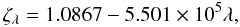 (F.2)with λ the wavelength in m. For the FUV band at 151.6 nm, ζ ≃ 1.0033. When ζ = 1, Eq. (F.1) is identical to the slab case (Eq. (8)). As we limit the computation of the face-on optical depth to the FUV band (see Sect. 7 for the extension to other wavelengths), we will not discuss the sandwich geometry further.
We also consider the case where dust is concentrated into clumps that are distributed following a Poisson distribution. In this case the relation between the attenuation and the optical depth is
 (F.3)with
  the average number of clouds along the line of sight, and τλc the optical depth of an individual cloud.
In Fig. F.1, we compare the effective attenuation for various geometries, versus the mean optical depth  .
.
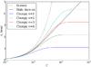 |
Fig. F.1
Attenuation versus the mean optical depth |
| Open with DEXTER | |
At low mean optical depths, all geometries yield the same attenuation. This means that the actual distribution of the dust, slab, clumpy, or even screen has little impact on the effective attenuation. However, from an optical depth of unity, there is a strong divergence. For a slab geometry (solid black line in Fig. F.1),  , whereas in the case of a clumpy distribution,
  , when
  . As a consequence, in the latter case the resulting attenuation curve becomes more grey as the optical depth increases. As we see, in the case of a distribution of very opaque clumps, the maximum attenuation is directly determined by the number of clumps and not by the optical depth of individual clouds.
F.2. Gas surface density and the optical depth for different geometries
We compute the relation between the gas surface density and the face-on optical depth for screen, and clumpy geometries to understand the impact of the assumed geometries on these relations.
If we assume that all galaxies in the sample have the same average number of clumps along the line of sight, we need  to be able to reproduce the observations. This is slightly larger than what was found by Holwerda et al. (2007) for a sample of 14 disk galaxies in the nearby Universe (
 ). Considering
  and
and  , we find the following relations between the optical depth and the gas surface density
  (F.4)and
 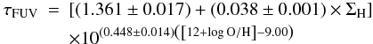 (F.5)for , and
  (F.6)and
 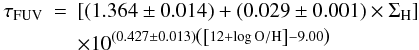 (F.7)for .
When we compare Eqs. (12) to (F.4) or (F.6), it yields very different optical depths. For instance, if we assume ΣH = 10 M⊙ pc-2, τFUV = 3.426 for a slab geometry and τFUV = 1.988 for a clumpy geometry with , reaching τFUV = 15.715 and τFUV = 6.704 respectively for ΣH = 100 M⊙ pc-2. This exemplifies strongly the model-dependence of such relations. In order to avoid biases, it is particularly important to use the same geometry when computing the attenuation as the one that was assumed for the relation between the gas surface density and the optical depth.
Appendix G: Inversion of the relation between the attenuation and the face-on optical depth for a slab geometry
In Sect. 5.1 we introduced the Lambert W function to express the face-on optical depth as a function of the attenuation (Eq. (9)). We indicate here how we have derived this equation and how the Lambert W function was introduced. First of all, we consider the equation we want to invert 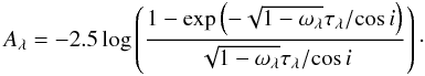 (G.1)Let
  . We easily get
 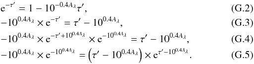 Using the W Lambert function, which gives the invert relation of
  , this is equivalent to
  (G.6)Redeveloping τ′ and rearranging slightly we obtain the final relation
  (G.7)
(G.7)
Appendix H: On the reproducibility of local LFs
As stated before, the aim of this exercise is not to reproduce exactly the LFs of nearby galaxies but to examine the impact of different gas surface density attenuation relations. Several intrinsic aspects of the simulations tend to incur biases affecting the LFs.
A first well-known problem is that semi-analytic relations can yield too much gas compared to what is observed in the local universe. To correct for this effect, following Obreschkow et al. (2009), we rescale the gas mass in each galaxy so that the total cold gas mass density at z = 0 is consistent with the value derived by Obreschkow & Rawlings (2009) , with
  normalised to the critical density for closure
  (H.1)H being the Hubble constant, and G the gravitational constant. For H = 73 km s-1 Mpc-1, ρcrit = 1.0 × 10⁻²⁶ kg m-3. We then rescale the cold gas masses from the simulation by multiplying them by the factor ξ-1, with ξ defined as
  (H.2)with
  the mean gas mass density of the simulation over the entire volume. We find that
  kg m-3, leading to ξ = 1.5. This is very similar to the factor 1.45 found by Obreschkow et al. (2009) for the De Lucia & Blaizot (2007) catalogue which was based on the Millennium simulation. In Fig. H.1, we show the Millennium-II cold gas mass luminosity.
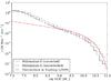 |
Fig. H.1
Mass function of the cold gas mass of the Millennium-II simulation (black lines), uncorrected (dashed line), and corrected (solid) for the mass excess. For comparison, the observed cold gas mass function derived by Obreschkow & Rawlings (2009) is shown in red. All functions have been rescaled to h = 0.73, following the Millennium-II simulation parameters (Boylan-Kolchin et al. 2009). |
| Open with DEXTER | |
At high mass, the model slightly underestimates the cold gas mass function compared to the observed one by Obreschkow & Rawlings (2009). Conversely, there is a very large excess of galaxies with a lower mass of gas, up to about 1 dex for log M(H) = 7.0.
The SFR distribution function, which is not affected by the attenuation, can also be compared to the observed functions in the local Universe.
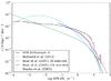 |
Fig. H.2
SFR function of the Millennium-II simulation (black line). For comparison, the Martin et al. (2005) function (cyan), the IR (red), and UV (blue) selected Buat et al. (2007) functions, and the Bothwell et al. (2011) functions observed in the local universe have also been plotted. All functions have been scaled to h = 0.73 and to a Chabrier (2003) IMF. |
| Open with DEXTER | |
In Fig. H.2, we show the observed SFR distribution functions of Martin et al. (2005),
Buat et al. (2007), and Bothwell et al. (2011). It turns out that the simulated SFR distribution function does not convincingly reproduce any of them. At the same time, there are significant differences among them. The difference is the smallest at relatively high SFR, but the difference rapidly increases under SFR = 10 M⊙ yr-1, at the level of the “knee” of the distribution. For an SFR < 1 M⊙ yr-1, the simulated SFR distribution function presents a much flatter slope than the observed ones. At the same time, Guo et al. (2011) remarked that the Millennium-II simulation produces a large fraction of non-star-forming dwarf galaxies compared to what is observed. This dearth of star-forming galaxies combined with the effect of the SFH − dwarf galaxies tend to have a more bursty SFH than large spirals which form stars at a steady rate − could explain this flattening of the slope. At optical and NIR wavelengths which are increasingly less sensitive to the exact SFH, this problem has a much weaker impact. Guo et al. (2011) showed that the Millennium-II simulations can reproduce convincingly the SDSS LFs derived by Blanton et al. (2005) in the g′, r′, i′, and z′ bands. However, in the star-formation tracing bands, these departures from the observed SFR distribution functions indicate that because we derive the extinction-free UV luminosity of each galaxy from the SFR as we saw in Sect. 9.1, we cannot compare directly our simulated UV and IR LFs with the observed ones. This is the reason why we do not attempt to carry out a comparison between our LFs and the observed ones.
© ESO, 2013
Current usage metrics show cumulative count of Article Views (full-text article views including HTML views, PDF and ePub downloads, according to the available data) and Abstracts Views on Vision4Press platform.
Data correspond to usage on the plateform after 2015. The current usage metrics is available 48-96 hours after online publication and is updated daily on week days.
Initial download of the metrics may take a while.