| Issue |
A&A
Volume 549, January 2013
|
|
|---|---|---|
| Article Number | A14 | |
| Number of page(s) | 16 | |
| Section | Stellar atmospheres | |
| DOI | https://doi.org/10.1051/0004-6361/201220240 | |
| Published online | 06 December 2012 | |
Online material
Appendix A: Analysis of the abundance corrections for lines of neutral atoms
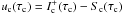
The temperature sensitivity of spectral lines originating from the neutral atoms of partially ionized species (e.g. Mg i, Ca i, Fe i) is governed by the Saha and Boltzmann equations, i.e. by changes of the degree of ionization and of the excitation of the line’s lower level. In the following, we develop a simplified model of the 3D– ⟨ 3D ⟩ abundance corrections, which result from horizontal fluctuations of the thermodynamical quantities.
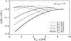 |
Fig. A.1
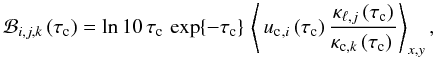
Abundance correction Δ3D − ⟨ 3D ⟩ , computed according to Eqs. (A.1)–(A.4), versus the difference between ionization and excitation potential, Eion − χ. Each curve corresponds to a different value of Eion. The thermodynamic variables θ(x,y) and pe(x,y) were taken from the 3D model at monochromatic optical depth log τ850 = −0.48, where the mean temperature is 3360 ± 140 K. The temperature dependence of the partition functions U0 and U1 has been neglected. |
| Open with DEXTER | |
The ratio of the total number of neutral atoms n0 (with
ionization energy Eion and partition function
U0) to the total number of singly ionized atoms
n1 (with partition function
U1) at temperature
T = 5040/θ and electron pressure
pe is given by Saha’s equation (see e.g. Gray 2005, Eq. (1.20))  (A.1)The
opacity of a line transition with lower level excitation potential χ is
proportional to the number of absorbing atoms (per unit mass) in this state of
excitation,
(A.1)The
opacity of a line transition with lower level excitation potential χ is
proportional to the number of absorbing atoms (per unit mass) in this state of
excitation,  (A.2)In the presence
of horizontal fluctuations of θ and pe, the
average line opacity is amplified with respect to the ⟨3D⟩ case by a factor
(A.2)In the presence
of horizontal fluctuations of θ and pe, the
average line opacity is amplified with respect to the ⟨3D⟩ case by a factor
 (A.3)where
⟨ . ⟩ x,y denotes horizontal averaging
at constant continuum optical depth τc. Assuming that
fluctuations of the continuum opacity and the source function can be neglected, the
abundance correction for weak lines can be estimated as
(A.3)where
⟨ . ⟩ x,y denotes horizontal averaging
at constant continuum optical depth τc. Assuming that
fluctuations of the continuum opacity and the source function can be neglected, the
abundance correction for weak lines can be estimated as 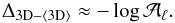 (A.4)Figure A.1 shows the result of computing
Δ3D − ⟨ 3D ⟩ according to Eqs. (A.1)–(A.4) for different
combinations of χ and Eion. The figure
illustrates how the curves Δ3D − ⟨ 3D ⟩ versus
Eion − χ change systematically as the
parameter Eion increases from 0 to 9 eV.
For Eion ≲ 6 eV, the neutral atoms are a minority species,
f ≪ 1, and we see from Eq. (A.2) that in this case
(A.4)Figure A.1 shows the result of computing
Δ3D − ⟨ 3D ⟩ according to Eqs. (A.1)–(A.4) for different
combinations of χ and Eion. The figure
illustrates how the curves Δ3D − ⟨ 3D ⟩ versus
Eion − χ change systematically as the
parameter Eion increases from 0 to 9 eV.
For Eion ≲ 6 eV, the neutral atoms are a minority species,
f ≪ 1, and we see from Eq. (A.2) that in this case 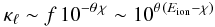 (A.5)depends
only on the difference (Eion − χ), such
that all curves with Eion ≲ 6 eV fall on top of each other.
As Eion increases further, the vertex of the curves moves
from (Eion − χ)max = 0 eV
to ≈ 4 eV to 9 eV as the ionization balance shifts from
⟨ f ⟩ x,y ≈ 0
(Eion = 0 eV) to ≈ 1
(Eion = 7 eV) to ≳ 1000
(Eion = 9 eV). In fact, it can be shown analytically that
(A.5)depends
only on the difference (Eion − χ), such
that all curves with Eion ≲ 6 eV fall on top of each other.
As Eion increases further, the vertex of the curves moves
from (Eion − χ)max = 0 eV
to ≈ 4 eV to 9 eV as the ionization balance shifts from
⟨ f ⟩ x,y ≈ 0
(Eion = 0 eV) to ≈ 1
(Eion = 7 eV) to ≳ 1000
(Eion = 9 eV). In fact, it can be shown analytically that
 (A.6)Admittedly, the
description of the abundance corrections developed above is severely simplified. It
ignores the fact that the line formation region is extended and that the location of its
center of gravity depends sensitively on Eion and
χ (cf. Figs. A.2, B.1, C.2). Also,
fluctuations of the continuum opacity and the source function were neglected.
Nevertheless, the systematics seen in Fig. A.1
provides a basic explanation of the detailed numerical results presented in Sect. 3.2, Fig. 3
(especially middle left panel).
(A.6)Admittedly, the
description of the abundance corrections developed above is severely simplified. It
ignores the fact that the line formation region is extended and that the location of its
center of gravity depends sensitively on Eion and
χ (cf. Figs. A.2, B.1, C.2). Also,
fluctuations of the continuum opacity and the source function were neglected.
Nevertheless, the systematics seen in Fig. A.1
provides a basic explanation of the detailed numerical results presented in Sect. 3.2, Fig. 3
(especially middle left panel).
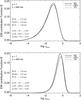 |
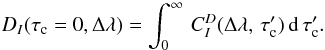
Fig. A.2
Disk-center (μ = 1) equivalent width contribution functions, ℬ(log τc), of a weak (artificial) Fe i line with excitation potential χ = 0 eV (top) and χ = 5 eV (bottom), at wavelengths λ 850 nm, evaluated according to the weak line approximation (Eqs. (B.5), (B.7)), for a single snapshot of the 3D model, the corresponding ⟨ 3D ⟩ average model, and the associated 1D LHD model used in this work. The contribution functions, originally defined on the monochromatic optical depth scale, have been transformed to the Rosseland optical depth scale. |
| Open with DEXTER | |
Appendix B: Analysis of the abundance corrections for high-excitation lines of ions
In the following, we analyze in some detail the abundance corrections derived for the high-excitation Fe ii lines, which are representative of the ionized atoms and show the largest 3D corrections (see Fig. 4). Evaluating the equivalent width contribution functions of this line in the 3D and the 1D models, we determine the physical cause of the abundance corrections. In particular, we can understand the sign of the 3D– ⟨ 3D ⟩ and ⟨ 3D ⟩ –1D corrections and explain why these corrections are so much smaller at λ 1600 nm than at λ 850 nm.
For simplicity, we consider only vertical rays (disk-center intensity) in a single snapshot from the 3D simulation, noting that the qualitative behavior of the abundance corrections is similar for intensity and flux, and does not vary much in time, i.e. the 3D– ⟨ 3D ⟩ correction is always strongly negative, while the ⟨ 3D ⟩ –1D correction is slightly positive at λ 850 nm.
B.1. Formalism
Following Magain (1986), the line depression
contribution function (for vertical rays, LTE),
 , is
defined in Linfor3D as
, is
defined in Linfor3D as  (B.1)where
τc is the continuum optical depth,
η(Δλ,τc) = κℓ(Δλ,τc)/κc(τc)
is the ratio of line opacity to continuum opacity,
(B.1)where
τc is the continuum optical depth,
η(Δλ,τc) = κℓ(Δλ,τc)/κc(τc)
is the ratio of line opacity to continuum opacity,
 is the difference between
outgoing continuum intensity and source function4, and
(τc + τℓ(Δλ))
is the total optical depth in the line; angle brackets
⟨.⟩x,y indicate horizontal averaging
at constant continuum optical depth. Note that η (and
τℓ) vary with wavelength position in
the line profile, Δλ, whereas τc and
uc can be considered as constant across the line
profile. Then the absolute line depression at any wavelength in the line profile is
is the difference between
outgoing continuum intensity and source function4, and
(τc + τℓ(Δλ))
is the total optical depth in the line; angle brackets
⟨.⟩x,y indicate horizontal averaging
at constant continuum optical depth. Note that η (and
τℓ) vary with wavelength position in
the line profile, Δλ, whereas τc and
uc can be considered as constant across the line
profile. Then the absolute line depression at any wavelength in the line profile is
 (B.2)Defining
further the equivalent width contribution function as
(B.2)Defining
further the equivalent width contribution function as 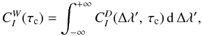 (B.3)the equivalent width
of the line is finally computed as
(B.3)the equivalent width
of the line is finally computed as 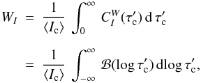 (B.4)where
⟨ Ic ⟩ is the horizontally averaged emergent continuum
intensity, and ℬ is defined as
(B.4)where
⟨ Ic ⟩ is the horizontally averaged emergent continuum
intensity, and ℬ is defined as  (B.5)In the limit of
weak lines, we can assume that
τℓ ≪ τc
over the whole line formation region, and Eqs. (B.1) and (B.3)
simplify to
(B.5)In the limit of
weak lines, we can assume that
τℓ ≪ τc
over the whole line formation region, and Eqs. (B.1) and (B.3)
simplify to  (B.6)and
 (B.7)where
 (B.8)In this weak
line limit, , and
hence
(B.8)In this weak
line limit, , and
hence  are
strictly proportional to the line opacity, and the equivalent width scales linearly
with the gf-value of the line (or the respective chemical abundance).
Then the 3D abundance corrections can simply be obtained from the equivalent widths as
are
strictly proportional to the line opacity, and the equivalent width scales linearly
with the gf-value of the line (or the respective chemical abundance).
Then the 3D abundance corrections can simply be obtained from the equivalent widths as
 (B.9)
(B.9)
B.2. Analysis of mixed contribution functions
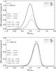 |
Fig. B.1
Disk-center (μ = 1) equivalent width contribution functions, ℬ(log τc), of a weak (artificial) Fe ii line with excitation potential χ = 10 eV, at wavelengths λ 850 nm (top) and λ 1600 nm (bottom), evaluated according to the weak line approximation (Eqs. (B.5), (B.7)), for a single snapshot of the 3D model, the corresponding ⟨ 3D ⟩ average model, and the associated 1D LHD model used in this work. The contribution functions, originally defined on the monochromatic optical depth scale, have been transformed to the Rosseland optical depth scale as a common reference. |
| Open with DEXTER | |
Figure B.1 compares the equivalent width contribution functions, ℬ, of a weak (artificial) Fe ii line with excitation potential χ = 10 eV at two wavelengths, λ 850 nm (top) and λ 1600 nm (bottom), for the 3D model, the corresponding ⟨ 3D ⟩ average model, and the associated 1D LHD model used in this work. For each of the different models the area below the corresponding curve is proportional to the equivalent width of the emerging line profile. At λ 850 nm, the equivalent width produced by the 3D model is significantly larger than that of the 1D LHD model, which in turn is significantly lager than that of the ⟨ 3D ⟩ model, assuming the same iron abundance in all cases. The abundance corrections derived with Eq. (B.9) are Δ3D − 1D = −0.33, Δ3D − ⟨ 3D ⟩ = −0.46, and Δ ⟨ 3D ⟩ − 1D = + 0.13 dex. These numbers are fully consistent with the results shown in Fig. 4. At λ 1600 nm, on the other hand, the equivalent widths obtained from the three different model atmospheres are obviously very similar; all abundance corrections are much smaller than those at λ 850 nm, again in basic agreement with the results shown in Fig. 4.
Figure B.1 also shows that the formation region of this high-excitation Fe ii line is well confined to a narrow region in the deep photosphere, mainly below τRoss = 1, where the degree of ionization of iron is changing rapidly with depth. As expected, the line originates from somewhat deeper layers at λ 1600 nm (minimum of H− opacity) than at λ 850 nm (maximum of H− opacity). According to Fig. 1, both the amplitude of the horizontal temperature fluctuations and the 1D– ⟨ 3D ⟩ temperature difference increase with depth in the range − 1 < log τRoss < + 1, such that they are larger in the line formation region at λ 1600 nm. Naively, one would thus expect the amplitude of the abundance corrections Δ3D − ⟨ 3D ⟩ and Δ ⟨ 3D ⟩ − 1D to be larger at λ 1600 nm than at λ 850 nm. However, this reasoning obviously fails. As we have seen before, the abundance corrections are found to be strikingly smaller at λ 1600 nm. Additional analysis is necessary to resolve this apparent contradiction.
To understand the origin of the abundance corrections, we need to understand the role
of the different factors that make up the contribution function ℬ, essentially
uc and
η0 = κℓ/κc.
The different behavior of these factors in the different types of models determines
the sign and amplitude of the abundance corrections. In the following, subscripts 1,
2, and 3 refer to the 1D LHD model, the ⟨ 3D ⟩ model, and the 3D model,
respectively. With this notation in mind, we define the mixed contribution functions
 (B.10)where
i = 1...3,
j = 1...3,
k = 1...3. The three mixed contribution functions
with three identical subscripts
i = j = k are thus the normal
contribution functions for the 1D, ⟨ 3D ⟩ , and 3D model, respectively. From each of
the ℬi,j,k we can compute an equivalent width according to
Eq. (B.4), which we denote as
Wi,j,k. The equivalent widths can then
be used to derive abundance corrections via
(B.10)where
i = 1...3,
j = 1...3,
k = 1...3. The three mixed contribution functions
with three identical subscripts
i = j = k are thus the normal
contribution functions for the 1D, ⟨ 3D ⟩ , and 3D model, respectively. From each of
the ℬi,j,k we can compute an equivalent width according to
Eq. (B.4), which we denote as
Wi,j,k. The equivalent widths can then
be used to derive abundance corrections via  (B.11)The numerical
evaluation of the relevant abundance corrections is compiled in Table B.1.
(B.11)The numerical
evaluation of the relevant abundance corrections is compiled in Table B.1.
Abundance corrections for the Fe ii line (χ = 10 eV) derived from mixed contribution functions ℬi,j,k at λ 850 and 1600 nm.
B.2.1. ⟨ 3D ⟩ –1D abundance corrections
With the help of Table B.1, the physical interpretation of the Δ ⟨ 3D ⟩ − 1D abundance correction is straightforward. Columns (6) and (7) show the effect of the different factors that contribute to the ⟨ 3D ⟩ –1D abundance correction. Owing to the different thermal structure of the two model atmospheres, all three factors, uc, κℓ, and κc change simultaneously, and the full correction is Δ ⟨ 3D ⟩ − 1D = Δ2,2,2,1, listed in the last row of the table as case (7). The other cases (1)–(6) refer to “experiments” where only one or two of the factors are allowed to change while the remaining factors are fixed to expose the abundance corrections due to the individual factors. Case (1), for example, shows the correction that would result for fixed opacities, κℓ(τc), κc(τc), accounting only for the differences in the source function gradient uc. Case (6) shows the complementary experiment where uc is fixed and both opacities are changing in accordance with the different thermodynamical conditions.
At λ 850 nm, the continuum opacity is dominated by H− bound-free absorption, which shows its maximum at this wavelength. The high-excitation Fe ii line forms around log τ850 ≈ + 0.7 (log τRoss ≈ + 0.6), i.e. significantly below continuum optical depth unity. At this depth, both the temperature and the temperature gradient are slightly lower in the ⟨ 3D ⟩ model than in the 1D model. As a consequence, both uc and κc decrease toward the ⟨ 3D ⟩ model, approximately by the same factor (see cases 1 and 4), and hence their effects cancel out. The highly temperature-dependent line opacity (∂log κℓ/∂θ ≈ − 10; θ = 5040/T) is thus the dominating factor and determines the total Δ ⟨ 3D ⟩ − 1D abundance correction (compare cases 2 and 7).
At λ 1600 nm, the situation is different. Here the continuum opacity is mainly due to H− free-free absorption. The important difference is that the temperature sensitivity of the H− free-free opacity is significantly higher than that of the H− bound-free absorption (see Fig. B.2). In the line formation region around log τ1600 ≈ + 0.15 (log τRoss ≈ + 0.85), the temperature sensitivity of κℓ and κc is now comparable, such that the ratio of both opacities is nearly the same in the two models. The corrections due to κℓ and κc are almost equal and of opposite sign (cases 2 and 4), and hence cancel out. At the same time, the source function gradient is very similar in both models, and thus the correction due to uc is small (case 1). The total Δ ⟨ 3D ⟩ − 1D abundance correction is therefore significantly smaller than at λ 850 nm (case 7).
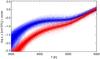 |
Fig. B.2
Continuous opacity due to H |
| Open with DEXTER | |


B.2.2. 3D– ⟨ 3D ⟩ abundance corrections
The physical interpretation of the Δ3D − ⟨ 3D ⟩ abundance correction proceeds along similar lines. Columns (3) and (4) of Table B.1 show the influence of the different factors that contribute to the 3D– ⟨ 3D ⟩ “granulation correction”. The three factors, uc, κℓ, and κc differ between the 3D and the ⟨ 3D ⟩ model due to the presence of horizontal fluctuations of the thermodynamical conditions at constant optical depth τc, which then lead to more or less nonlinear fluctuations of the factors that make up the contribution function. The full correction, Δ3D − ⟨ 3D ⟩ = Δ3,3,3,2, allows for fluctuations in all three factors and is listed in the last row of the table as case (7). The other cases (1)–(6) refer to “experiments” where the fluctuations are artificially suppressed for one or two of the factors to study the impact of the fluctuations of the individual factors on the resulting the abundance correction. For example, case (5) shows the correction that would result if the fluctuations of the line opacity, κℓ(τc), were suppressed. case (2) shows the complementary experiment where only κℓ(τc) is allowed to fluctuate, while uc and κc are fixed.
At λ 850 nm, our weak Fe ii line is strongly enhanced in the 3D model due to the nonlinear fluctuations of the line opacity. The fluctuations lead to a line enhancement, and hence to negative 3D– ⟨ 3D ⟩ abundance corrections, whenever ⟨ κℓ(T) ⟩ x,y > κℓ( ⟨ T ⟩ x,y), which happens to be the case as κℓ ∝ exp { − E/kT } (roughly speaking because ∂2κℓ/∂T2 > 0). As can be deduced from the comparison of cases (2) and (7), suppression of the fluctuations of both uc and κc does not change the resulting 3D abundance correction. We can furthermore see that the fluctuations of uc enhance the nonlinearity of the fluctuations of κℓ (case 3) and that the fluctuations of κc diminish the nonlinearity of the fluctuations of κℓ (case 6). We conclude that the fluctuations of uc and κc must be substantial, but essentially linear, such that they do not produce any significant abundance corrections on their own (cases 1, 4, and 5).
At λ 1600 nm, the continuum opacity κc is lower than at λ 850 nm, and our weak Fe ii line forms at somewhat deeper layers where the temperature is higher. Equally important, the temperature sensitivity of κc is distinctly higher at λ 1600 nm than at λ 850 nm, as is demonstrated in Fig. B.2. This fact is the key to understanding the drastically smaller abundance corrections found at λ 1600 nm.
Comparing the effect of the line opacity fluctuations for the two wavelengths (case 2), we see that the corresponding abundance correction is significantly smaller at λ 1600 nm. This result is unexpected, because according to Fig. 1 the temperature fluctuations, δTrms, ought to be larger in the deeper layers where the near-IR line forms, which in turn should lead to more nonlinear fluctuations of the line opacity and hence larger abundance corrections at λ 1600 nm compared to λ 850 nm.
Further investigations revealed that the opposite is true. The point is that we
have to distinguish between fluctuations at constant Rosseland optical depth,
τRoss, and fluctuations at constant monochromatic
optical depth, τc, which are relevant in the present
context. In fact, the higher temperature sensitivity of the continuum opacity at
λ 1600 nm reduces the amplitude of the temperature fluctuations
at constant continuum optical depth τ1600 with respect
to the fluctuations at constant τ850, as illustrated in
Fig. B.3 (top panel). The degree of
nonlinearity of the line opacity fluctuations, as measured by the ratio of average
line opacity to line opacity at mean temperature,
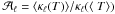 ,
is shown in the bottom panel of Fig. B.3. Over
the whole depth range, the nonlinearity of the
κℓ fluctuations is higher at
constant τ850 than at constant
τ1600. Remarkably,
,
is shown in the bottom panel of Fig. B.3. Over
the whole depth range, the nonlinearity of the
κℓ fluctuations is higher at
constant τ850 than at constant
τ1600. Remarkably,
 increases
toward lower temperatures, even though the amplitude of the temperature fluctuations
decreases with height. This is because the temperature sensitivity
of κℓ increases strongly as
Fe ii becomes a minority species at lower T (cf.
Fig. 2). The fact that
is significantly higher for the red line at λ 850 nm than for the
near-IR line at λ 1600 nm explains the wavelength dependence of the
abundance corrections found for case (2), Cols. (3) and (4).
increases
toward lower temperatures, even though the amplitude of the temperature fluctuations
decreases with height. This is because the temperature sensitivity
of κℓ increases strongly as
Fe ii becomes a minority species at lower T (cf.
Fig. 2). The fact that
is significantly higher for the red line at λ 850 nm than for the
near-IR line at λ 1600 nm explains the wavelength dependence of the
abundance corrections found for case (2), Cols. (3) and (4).
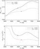 |
Fig. B.3
Amplitude of the (relative) temperature fluctuations,
δTrms/ ⟨ T ⟩
(top), and ratio of average line opacity to line opacity at
mean temperature, |
| Open with DEXTER | |
Comparing cases (2) and (6) for the near-IR line, we see that the abundance correction essentially vanishes when combining the fluctuations of the line opacity with the fluctuations of the continuum opacity. We note that the fluctuations of κc are significantly larger at log τ1600 = 0.15, where the near-IR line forms, than at log τ850 = 0.7, where the red line forms, even though the temperature fluctuations are lower (see Fig. B.3). This is again a consequence of the enhanced temperature sensitivity of the continuum opacity at λ 1600 nm (Fig. B.2). It thus happens that the abundance corrections due to the fluctuations of the continuum opacity and the line opacity, respectively, are comparable (compare cases 2 and 4). The net result is a cancelation of the two effects. The total Δ3D − ⟨ 3D ⟩ abundance correction λ 1600 nm is therefore small.
B.3. Saturation effects
So far we have considered the abundance corrections for the limiting case of weak, unsaturated lines. In this limit, the abundance corrections are independent of the equivalent width of the line and of the microturbulence parameter ξmic chosen for the spectrum synthesis with the 1D models. Figure B.4 shows how the results change if saturation effects are fully taken into account, again for the example of the high-excitation Fe ii line.
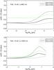 |
Fig. B.4
Total 3D abundance correction Δ3D−1D for the artificial Fe ii line with excitation potential χ = 10 eV at λ 850 nm (top) and λ 1600 nm (bottom) as a function of the equivalent width obtained from the 3D model. The fainter (green) curves and the thicker (black) curves refer to the intensity (μ = 1) and flux spectrum, respectively. The abundance corrections have been computed for three different values of the microturbulence parameter used with the 1D model, ξmic = 0.0 (dotted), 1.0 (solid), and 2.0 km s-1 (dashed lines). The weak line limit coincides with the horizontal part of the curves at low log W3D. |
| Open with DEXTER | |
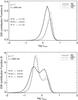 |
Fig. B.5
Disk-center (μ = 1) equivalent width contribution functions, ℬ(log τc), of a weak (top) and strong (bottom) Fe ii line with excitation potential χ = 10 eV, at λ 850 nm. The contribution functions have been computed for a single snapshot of the 3D model (solid), the corresponding ⟨ 3D ⟩ average model (dashed), and the associated 1D LHD model (dotted) used in this work. They have been transformed from the monochromatic to the Rosseland optical depth scale. In all cases, the saturation factor exp { − τℓ } is properly taken into account (see Eq. (B.1)). |
| Open with DEXTER | |
Obviously, the total 3D abundance correction, Δ3D − 1D, depends strongly
on both the assumed value of ξmic and on the line
strength, W3D. We notice that this holds even for very
weak lines, and conclude that even the weakest lines used for this study are already
partly saturated. Plotting log W3D versus
log gf reveals that the curve-of-growth is linear, and thus
saturation effects can be safely ignored as long as the equivalent width of the line
is below  pm at
λ 850 nm (
pm at
λ 850 nm ( pm at
λ 1600 nm). As soon as this line becomes detectable, it is no
longer on the linear part of the curve-of-growth. This extreme behavior is of course
related to the extreme temperature sensitivity of this high-excitation line, which
changes the line-to-continuum opacity ratio from η ≪ 1 to
η ≫ 1 within the line formation region. This is especially true at
λ 850 nm, where the continuum opacity is less temperature
dependent (see above). The partial saturation of weak lines is not a particular
property of the 3D model, but is seen in 1D models, too.
pm at
λ 1600 nm). As soon as this line becomes detectable, it is no
longer on the linear part of the curve-of-growth. This extreme behavior is of course
related to the extreme temperature sensitivity of this high-excitation line, which
changes the line-to-continuum opacity ratio from η ≪ 1 to
η ≫ 1 within the line formation region. This is especially true at
λ 850 nm, where the continuum opacity is less temperature
dependent (see above). The partial saturation of weak lines is not a particular
property of the 3D model, but is seen in 1D models, too.
The top panel of Fig. B.5 shows the equivalent width contribution functions ℬ(τRoss) of the same weak Fe ii line (χ = 10 eV, λ 850 nm) as in Fig. B.1 (top), but now including the saturation factor exp { − τℓ } (see Eq. (B.1)). Comparison with Fig. B.1 (top) demonstrates that including the saturation factor reduces the equivalent width from W3D ≈ 0.61 pm to W3D ≈ 0.17 pm). Moreover, all contribution functions are shifted to slightly higher layers because of the presence of saturation effects. The upward shift is more pronounced for the 3D contribution function, because of the strongly nonlinear fluctuations of the saturation factor exp { − τℓ } . As a result, ℬ(3D) now becomes smaller than ℬ( ⟨ 3D ⟩ ) and ℬ(1D) in the deepest part of the line-forming region. Therefore, the ratio of 3D to 1D equivalent width becomes smaller than in the weak line limit, where ℬ(3D) > ℬ(1D) over the whole optical depth range. Hence, the total 3D abundance correction, Δ3D − 1D, becomes less negative if saturation is taken into account.
If the line strength is increased even more, the contribution functions become wider and extend to higher atmospheric layers, as shown in the bottom panel of Fig. B.5. Recalling that the equivalent width contribution function is a superposition of the line depression contribution functions for the individual wavelength positions in the line profile, it seems evident that the double peak structure is related to the contributions of the line core (left peak) and of the extended line wings (right peak). Test calculations confirm this interpretation. Proceeding form the top to the bottom of the line formation region, the difference ℬ(3D) − ℬ(1D) changes sign from positive to negative to positive to negative. Because the contributions of the different layers to the abundance correction cancel partially, a straightforward interpretation of the resulting abundance correction becomes difficult. In principle, a detailed analysis of the line depression contribution functions at individual wavelengths might lead to further insights. Noting, however, that the situation becomes even more complicated when considering flux spectra (involving inclined rays), we have some doubts that such an investigation is worthwhile.
Appendix C: Molecule concentrations, line opacities, and height of formation
The equilibrium number density of diatomic molecules with constituents
A and B,
NAB, is given by the Saha-like relation
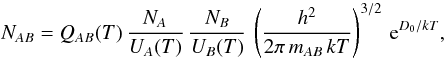 (C.1)where
NA and
NB are the number densities (per unit
volume) of free neutral atoms (in the ground state) of elements A and
B, with partition functions
UA and
UB, respectively; the molecule is
characterized by its mass, mAB, its
partition function, QAB, and its
dissociation energy D0 (cf. Cox 2000). Defining the number densities per unit mass as
Xi = Ni/ρ,
where ρ is the mass density, we obtain
(C.1)where
NA and
NB are the number densities (per unit
volume) of free neutral atoms (in the ground state) of elements A and
B, with partition functions
UA and
UB, respectively; the molecule is
characterized by its mass, mAB, its
partition function, QAB, and its
dissociation energy D0 (cf. Cox 2000). Defining the number densities per unit mass as
Xi = Ni/ρ,
where ρ is the mass density, we obtain  (C.2)Figure C.1 shows the number densities of our selection of
diatomic molecules (normalized to the total number of carbon nuclei,
NAB/ ∑ NC = XAB/ ∑ XC)
as a function of Rosseland optical depth in the 1D LHD model used in this work. In the
photosphere (log τRoss < 0), essentially all carbon
is locked up in CO. The decrease of XOH,
XNH, XCN toward lower optical
depths is a consequence of the density factor ρ in Eq. (C.2). The destruction of all molecules
beyond τRoss ≈ 1 is due to the Boltzmann factor
exp { D0/kT } ; a higher dissociation
energy corresponds to a steeper drop of the molecule concentration with
T.
(C.2)Figure C.1 shows the number densities of our selection of
diatomic molecules (normalized to the total number of carbon nuclei,
NAB/ ∑ NC = XAB/ ∑ XC)
as a function of Rosseland optical depth in the 1D LHD model used in this work. In the
photosphere (log τRoss < 0), essentially all carbon
is locked up in CO. The decrease of XOH,
XNH, XCN toward lower optical
depths is a consequence of the density factor ρ in Eq. (C.2). The destruction of all molecules
beyond τRoss ≈ 1 is due to the Boltzmann factor
exp { D0/kT } ; a higher dissociation
energy corresponds to a steeper drop of the molecule concentration with
T.
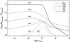 |
Fig. C.1
Number density of different molecules, normalized to the total number density of carbon (sum over all molecules and ionization states) as a function of the Rosseland optical depth in the 1D LHD model. |
| Open with DEXTER | |
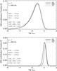 |
Fig. C.2
Same as Fig. A.2, but for two weak (artificial) molecular lines: a CO line with excitation potential χ = 0 eV (top) and a C2 line with χ = 4 eV (bottom), both at wavelength λ 850 nm. |
| Open with DEXTER | |
The opacity of a line with lower transition level energy χ, is
proportional to
XAB/QQB exp { − χ/kT } ,
and thus the line opacity per unit mass can be written as  (C.3)where
θ = 5040/T, and the temperature dependence of the
partition functions UA and
UB has been ignored; the molecular
partition function QAB cancels out.
(C.3)where
θ = 5040/T, and the temperature dependence of the
partition functions UA and
UB has been ignored; the molecular
partition function QAB cancels out.
If both atoms A and B are majority species (e.g. H,
N, O for the conditions in our red giant atmosphere), then
XA and
XB are constant, and the temperature
dependence of the line opacity is given by 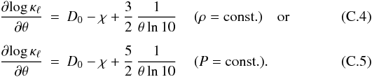 In
general, the temperature dependence of the molecular line opacity is more complicated,
because XA and/or
XB are more or less strongly
temperature dependent due to ionization and/or formation of different molecules. In our
red giant atmosphere, for example, the concentration of carbon atoms is controlled by
the formation of CO molecules. This leads to a strong increase
of κℓ with temperature
(∂log κℓ/∂θ < 0)
for CH and C2 at τRoss < 1, such that
these molecules can only form in a narrow region centered around
log τRoss ≈ 0 (see Fig. C.2).
In
general, the temperature dependence of the molecular line opacity is more complicated,
because XA and/or
XB are more or less strongly
temperature dependent due to ionization and/or formation of different molecules. In our
red giant atmosphere, for example, the concentration of carbon atoms is controlled by
the formation of CO molecules. This leads to a strong increase
of κℓ with temperature
(∂log κℓ/∂θ < 0)
for CH and C2 at τRoss < 1, such that
these molecules can only form in a narrow region centered around
log τRoss ≈ 0 (see Fig. C.2).
Finally, we point out that the molecular lines form in the same height range as the lines of neutral atoms and ions.
Figure C.2 displays the contribution functions for the most extreme examples. The ground state CO line (top panel) shows the most extended formation region, centered around log τRoss ≈ − 1. The contribution function of this line is almost identical to that of the ground state Fe i line shown in Fig. A.2. The high-excitation C2 line (bottom panel) originates from a very narrow formation region located in the deep photosphere around log τRoss ≈ 0. The contribution functions of the other molecular lines considered in this study lie somewhere in between these two extremes; the entire formation region of the molecular lines is always inside the height range covered by our model atmospheres.
© ESO, 2012
Current usage metrics show cumulative count of Article Views (full-text article views including HTML views, PDF and ePub downloads, according to the available data) and Abstracts Views on Vision4Press platform.
Data correspond to usage on the plateform after 2015. The current usage metrics is available 48-96 hours after online publication and is updated daily on week days.
Initial download of the metrics may take a while.