| Issue |
A&A
Volume 540, April 2012
|
|
|---|---|---|
| Article Number | A16 | |
| Number of page(s) | 41 | |
| Section | Galactic structure, stellar clusters and populations | |
| DOI | https://doi.org/10.1051/0004-6361/201016384 | |
| Published online | 16 March 2012 | |
Online material
Description of the HST additional archive data sets used in this paper, other than those from GO-10775.
Fraction of binaries with mass ratio q > 0.5, q > 0.6 and q > 0.7, and total fraction of binaries measured in different regions.
Collection of literature binary fraction estimates.
Appendix A: Reliability of the measured binary fraction
In this appendix we investigate whether the fraction of binaries with q > 0.5 that we measured with the procedure described in Sect. 4 are reliable or are affected by any systematic uncertainty due to the method we used. The basic idea of this test consists of simulating a number of CMDs with a given fraction of binaries, measuring the fraction of binaries in each of them, and comparing the added fraction of binaries with the measured ones.
Simulation of the CMD. We started by using artificial stars to simulate a CMD made of single stars following the procedure already described in Sect. 4.2. To simulate binary stars to be added to the simulated CMD we adopted the following procedure:
-
we selected a fraction
 of single stars equal to the fraction of binaries that we want to add to the CMD and derived their masses by using the Dotter et al. (2007) mass-luminosity relation. In our simulations we assumed the values of
  , 0.10, 0.30, and 0.50;
 -
for each of them, we calculated the mass ℳ2 = q × ℳ1 of the secondary star and obtained the corresponding mF814W magnitude. Its color was derived by the MSRL. For simplicity we assumed a flat mass-ratio distribution;
-
finally, we summed up the F606W and F814W fluxes of the two components, calculated the corresponding magnitudes, added the corresponding photometric error, and replaced the original star in the CMD with this binary system.
As an example, in the upper panels of Fig. A.1 we show the artificial star CMD made of single stars only (left panel), and the CMD where we added a fraction  of binaries (right panel), for the case of NGC 2298.
Simulation of the differential reddening. To probe how well the reddening correction works, we considered a simple model. The simulation of the differential reddening suffered by any single star is far from trivial as we have poor information on the structure of the interstellar medium between us and each GC. For simplicity, in this work we assumed that reddening variations are related to the positions (X, Y) of each stars by the following relations:


 Here XMIN,MAX and YMIN,MAX are the minimum and the maximum values of the coordinates X and Y, C1 is a free parameter that determines the maximum amplitude E(B − V) variation, and C2 governs the number of differential reddening peaks within the field of view.
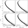 |
Fig. A.1
Artificial stars CMD for NGC 2298 (upper-left) and simulated CMD with a fraction of |
| Open with DEXTER | |
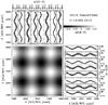 |
Fig. A.2
Bottom-left: Map of differential reddening added to the simulated CMD of NGC 2298. The gray levels indicate the reddening variations as indicated in the upper-right panel. Upper-left and bottom-right panels show ΔE(B − V) as a function of the Y and X coordinate respectively for stars into 8 vertical and horizontal slices. |
| Open with DEXTER | |
In this work, we used for each GC the value of C1 that ranges from 0.005 to 0.05 to account for the observed reddening variation in all the GCs, while we arbitrarily assumed three values of C2 = 3, 5, and 8 to reproduce three different fine-scales of differential reddening. As an example, in Fig. A.2 we show the map of differential reddening added to the simulated CMD of NGC 2298 that is obtained by assuming C1 = 0.025 and C2 = 5.
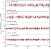 |
Fig. A.3
Difference between the measured fraction of binaries and the fraction of binaries in input as a function of the parameter C1 for four difference values of the input binary fraction. Black lines indicate the average difference. Red circles, gray triangles and black crosses indicate simulations with C2 = 3, 5, and 8 respectively. |
| Open with DEXTER | |
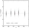 |
Fig. A.4
Fractions of binaries per unit q measured in five mass-ratio intervals as a function of q for all the simulated GCs. To compare the q distribution in simulated clusters with different fraction of binaries, we divided νbin by two times the fraction of binaries with q > 0.5. For clarity, black points have been randomly scattered around the corresponding q value. The means normalized binary fractions in each mass-ratio bin are represented by red points with error bars, while the gray line is the best fitting line, whose slope is quoted in the inset. |
| Open with DEXTER | |
Then, we have transformed the values of ΔE(B − V) corresponding to the position of each stars into ΔAF606W, and ΔAF814W and added these absorption variations to the F606W and the F814W magnitudes. The CMD obtained after we added differential reddening is shown in the bottom left panel of Fig. A.1 for NGC 2298. We applied to this simulated CMD the procedure to correct for differential reddening described in Sect. 3.1 and obtain the corrected CMD shown in the bottom right panel. For each of these binary-enhanced simulated CMD, we also generated a CMD made of artificial stars by following the approach described in Sect. 4.2. In our investigation we did not account for field stars. For each combination of the and C2 we have simulated 200 CMDs with random values of the C1.
Measurements of the binary fraction. Finally, we used the procedure of Sect. 4 to measure the fraction of binaries with mass ratio q > 0.5 defined as:
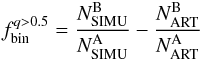 where
where  and
and  are the numbers of stars in the regions A and B in the CMD, as defined in Fig. 11 in the binary-enhanced simulated CMD and
  and
and  the numbers of stars in the same regions of the artificial stars CMD.
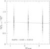 |
Fig. A.5
Fraction of binaries with q > 0.5 in three magnitude intervals as a function of ΔmF814W for all the simulated GCs. To compare the measured fraction of binaries in different clusters we have divided the measured binary fractions in each magnitude interval by the value of |
| Open with DEXTER | |

Results are shown in Fig. A.3 where we plotted the difference between the measured and the input fraction of binaries versus the parameter C1 for four difference values of the input binary fraction. We found that, for input binary fraction of 0.05, 0.10 and 0.30, the average difference are negligible (<0.5%), as indicated by the the black lines and the numbers quoted in the inset. In the case of a large binary fraction ( ) the measured fraction of binaries with q > 0.5 is systematically underestimated by ~0.03. Apparently our results do not depend on the value of the parameter C2. Simulations with C2 = 3, 5, and 8 (indicated in Fig. A.3 with red circles, gray triangles, and black crosses, respectively) give indeed the same average differences. Our comparison between the fraction of binaries added to the simulated CMD and the measured ones demonstrate that the fraction of binaries determined in this work and listed in Table 2 are not affected by any significant systematic errors related to the procedure we adopted.
We have also determined the fraction of binaries in five mass-ratio intervals by following the approach described in Sect. 5.1 for real stars. To this aim, we have divided the region B of the CMD defined in Sect. 11 into five subregions as illustrated in Fig. 22 for real stars. The size of each region is chosen in such a way that each of them covers a portion of the CMD with almost the same area. The resulting mass-ratio distribution is shown in Fig. A.4, where we have plotted the fraction of binaries per unit q as a function of the mass ratio. As already done in the case of real stars, to compare the mass-ratio distribution in simulated CMDs with different binary fraction, we have divided νbin by two times the measured fraction of binaries with q > 0.5. The best fitting gray line closely reproduce the flat mass-ratio distribution in input with νbin = 1.
Finally we have measured in the simulated CMDs the fraction of binaries with q > 0.5 in three intervals [0.75,1.75], [1.75,2.75], and [2.75,3.75] F814W magnitudes below the MSTO. To do this we used the procedure already described in Sect. 5.4 for real stars and we have normalized the  value measured in each magnitude bin by the fraction of binaries with q > 0.5 measured in the whole interval between 0.75 and 3.75 F814W magnitudes below the MSTO. Results are shown in
Fig. A.5 where we have plotted the normalized binary fractions as a function of ΔmF814W. The best-fitting gray line is nearly flat, and well reproduces the input magnitude distribution.
These tests demonstrate that both the mass-ratio distribution determined in Sect. 5.1 for the 59 GCs studied in this work and shown in Fig. 25 as well as the binary fractions measured in different magnitude intervals in Sect. 5.4 are not biased by significant systematic errors related to the procedure we adopted.
Appendix B
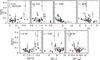 |
Fig. B.1
Fraction of binaries with q > 0.5 in the core as a function of some parameters of their host GCs. Clockwise: ellipticity, central concentration, central velocity dispersion, logarithm of the central luminosity density, half-mass and core relaxation timescale, and metallicity. In each panel we quoted the Pearson correlation coefficient (r). PCC clusters are marked with red crosses and are not used to calculate r (see text for details). |
| Open with DEXTER | |
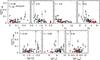 |
Fig. B.2
As in Fig. B.1 for the rC − HM sample. |
| Open with DEXTER | |
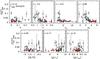 |
Fig. B.3
As in Fig. B.1 for the roHM sample. |
| Open with DEXTER | |
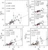 |
Fig. B.4
Upper-left: fraction of binaries with q > 0.5 in the core as a function of the absolute visual magnitude of the host GC. Dashed line is the best fitting straight line whose slope (s) and intercept (i) are quoted in the figure together with the Pearson correlation coefficient (r). PCC clusters are marked with red crosses and are not used to calculate neither the best-fitting line nor r. For completeness in the upper-right panels we show the same plot for the fraction of binaries with q > 0.6, and q > 0.7. Lower panels: fraction of binaries with q > 0.5 in the rC − HM (left) and roHM (right) sample as a function of MV. |
| Open with DEXTER | |
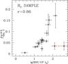 |
Fig. B.5
Fraction of binaries with q > 0.5 as a function of the BSS frequency in the core. PCC GCs are marked with red points. |
| Open with DEXTER | |
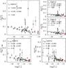 |
Fig. B.6
Fraction of binaries with q > 0.5, q > 0.6, and q > 0.7 in the rC region (upper panels) and fraction of binaries with q > 0.5 in the rC − HM and roHM regions (bottom panels) as a function of the collisional parameter (Γ∗). The adopted symbols are already defined in Fig. B.4. |
| Open with DEXTER | |
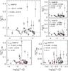 |
Fig. B.7
As in Fig. B.6. In this case we used the encounter frequency adopted by Pooley & Hut (2006) in the approximation used for virialized systems. |
| Open with DEXTER | |
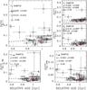 |
Fig. B.8
Fraction of binaries with q > 0.5, q > 0.6, and q > 0.7 in the rC region (upper panels) and fraction of binaries with q > 0.5 in the rC−HM and roHM regions (bottom panels) as a function of the relative age measured by Marín-Franch et al. (2009). The adopted symbols are already defined in Fig. B.4. |
| Open with DEXTER | |
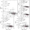 |
Fig. B.9
As in Fig. B.8 but in this case we used the age measures from Salaris & Weiss (2002) and De Angeli et al. (2005). |
| Open with DEXTER | |
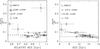 |
Fig. B.10
Fraction of binaries with q > 0.5 in the rC sample for low density clusters (log (ρ0) < 2.75) as a function of the relative age from Marín-Franch et al. (2009) (left panel) an absolute age from Salaris & Weiss (2002) and De Angeli et al. (2005) (right panel). |
| Open with DEXTER | |
 |
Fig. B.11
Fraction of binaries with q > 0.5 as a function of the temperature of the hottest HB stars (bottom), the HB morphology index (middle), and the median color difference between the HB and the RGB (top). |
| Open with DEXTER | |
© ESO, 2012
Current usage metrics show cumulative count of Article Views (full-text article views including HTML views, PDF and ePub downloads, according to the available data) and Abstracts Views on Vision4Press platform.
Data correspond to usage on the plateform after 2015. The current usage metrics is available 48-96 hours after online publication and is updated daily on week days.
Initial download of the metrics may take a while.