


| Issue |
A&A
Volume 712, August 2026
|
|
|---|---|---|
| Article Number | A1 | |
| Number of page(s) | 12 | |
| Section | Cosmology (including clusters of galaxies) | |
| DOI | https://doi.org/10.1051/0004-6361/202555553 | |
| Published online | 30 July 2026 | |
Robustness of pairwise kinematic Sunyaev–Zel’dovich effect to optical-cluster-selection bias
1
University Observatory, Faculty of Physics, Ludwig-Maximilians-Universität, Scheinerstr. 1 81679 Munich, Germany
2
Max-Planck-Institut für extraterrestrische Physik (MPE), Giessenbachstrasse 1, 85748 Garching bei München, Germany
3
Institute of Astronomy and Astrophysics, Academia Sinica (ASIAA), Taipei 10617, Taiwan
4
Excellence Cluster ORIGINS, Boltzmannstr. 2 85748 Garching, Germany
5
Department of Physics and Astronomy, University of Pennsylvania, Philadelphia PA 19104, USA
6
Max-Planck-Institut für Astrophysik, Karl-Schwarzschild-Strasse 1 85741 Garching, Germany
7
Department of Astronomy and Astrophysics, University of Chicago, Chicago IL 60637, USA
8
Department of Physics, Southern Methodist University, Dallas TX 75205, USA
9
European Southern Observatory, Karl Schwarzschildstrasse 2, 85748 Garching bei München, Germany
10
Department of Physics, University of Arizona, 1118 East Fourth Street Tucson AZ 85721, USA
★ Corresponding author: This email address is being protected from spambots. You need JavaScript enabled to view it.
Received:
16
May
2025
Accepted:
1
April
2026
Abstract
The pairwise kinematic Sunyaev–Zel’dovich (kSZ) effect measures both the pairwise motion between galaxy groups and clusters and the amount of gas within them, providing a tracer for cosmic growth. To interpret the cosmological information in the kSZ measurements, it is crucial to understand the optical-cluster-selection bias on the kSZ observables. Line-of-sight structures that contribute to both the optical observable (e.g., richness) and the cosmological signal can induce a correlation between these two quantities at a fixed cluster mass. The selection bias arising from this correlation is a key systematic effect for cosmological analyses. For cosmological observables such as cluster abundance and weak lensing, controlling this selection bias may help explain the tension between the DES-Y1 results and the Planck constraints. In order to test for a kSZ effect equivalent of such a bias, we adopted an alternative mock richness based on galaxy counts within cylindrical volumes along the line of sight. We applied the cylindrical count method to hydrodynamical simulations across a wide range of galaxy-selection criteria, assigning richness consistent with DES-Y1 to the mock clusters. When comparing optically selected clusters to mass-selected halos, we find no significant bias on pairwise kSZ signals, pairwise velocities, or optical depth within our uncertainty limits of approximately 16, 10, and 8%, respectively.
Key words: galaxies: clusters: general / galaxies: clusters: intracluster medium / cosmic background radiation / large-scale structure of Universe
© The Authors 2026
 Open Access article, published by EDP Sciences, under the terms of the Creative Commons Attribution License (https://creativecommons.org/licenses/by/4.0), which permits unrestricted use, distribution, and reproduction in any medium, provided the original work is properly cited.
This article is published in open access under the Subscribe to Open model. This email address is being protected from spambots. You need JavaScript enabled to view it. to support open access publication.
1. Introduction
During the growing process of large-scale structure, matter flows toward gravitational potential wells, eventually forming dense objects such as galaxy clusters. Measurements of the motions of material therefore provide direct insight into cosmic growth and offer constraints on cosmological physics – including dark energy – that are complementary to those from matter-density tracers.
Although direct spectroscopic observation of the peculiar velocity of galaxy clusters is challenging due to cosmic expansion, several methods have been developed to extract this information. The pairwise kinematic Sunyaev–Zel’dovich (kSZ) effect is one of the cosmic-growth tracers (Ferreira et al. 1999; Hand et al. 2012). The kSZ effect is a velocity-induced change in the cosmic microwave background (CMB) temperature, arising from the interaction of CMB photons with the bulk motion of ionized gas in the intra-cluster medium (ICM; Sunyaev & Zeldovich 1980). The signal is proportional to the line-of-sight peculiar velocity and the number density of the electrons, providing an approach for measuring the peculiar motion and the distribution of baryons. Two clusters tend to move toward each other due to gravity, leading to a net CMB temperature difference for the pairs, which is known as the pairwise kSZ signal. The pairwise kSZ signal can be expressed as the product of the mean optical depth,  of the cluster sample, and the mean relative pairwise velocity, v12 (Hand et al. 2012; Soergel et al. 2016),

where TpkSZ is the net deviation on the temperature of the CMB blackbody spectrum, TCMB. The pairwise kSZ effect provides a tool for distinguishing between models of acceleration of the cosmic expansion rate and for constraining the cosmic total neutrino mass (Mueller et al. 2015, 2014). The dependence of pairwise kSZ signals on the cosmic growth rate, f, and the present-day root-mean-square of matter density fluctuations, σ, is fσ2. This is complementary to other growth tracers such as redshift space distortions, which depend on fσ.
The kSZ signals also trace the distribution of baryons associated with dark-matter halos via the optical depth, τ, which is highly sensitive to the baryonic feedback processes in galaxy groups and cluster halos. The amount of baryonic feedback is a crucial systematic in modern weak lensing cosmology, especially in evaluating the significance of a potential tension between S8 measurements (Chisari et al. 2019; McCarthy et al. 2024; Bigwood et al. 2024). Recent analyses comparing stacked kSZ profiles of massive galaxies with hydrodynamical simulations suggest a scenario with more aggressive feedback than previously assumed (Hadzhiyska et al. 2024; Bigwood et al. 2024; McCarthy et al. 2024).
Since the initial measurement by Hand et al. (2012) of the pairwise kSZ effect, the detection significance has reached a level of more than 9σ (Calafut et al. 2021; Chen et al. 2022; Li et al. 2024; Hadzhiyska et al. 2025; Gong et al. 2025). Most past works cross-matched optical large surveys with CMB images, taking advantage of the large sample size of optical galaxies. There are two main approaches to identify proxies for the centers of massive groups and clusters: one assumes that a significant fraction of luminous galaxies are group and cluster centrals (Hand et al. 2012; Planck Collaboration XXXVII 2015; De Bernardis et al. 2017; Sugiyama et al. 2018; Calafut et al. 2021; Hadzhiyska et al. 2025; Gong et al. 2025), while the other applies group- and cluster-finding algorithms (Soergel et al. 2016; Chen et al. 2022; Schiappucci et al. 2023; Li et al. 2024). Throughout this paper, we refer to these algorithm-selected systems as “optical clusters”, although their mass range includes galaxy groups and clusters. Compared to luminous galaxies, algorithm-selected clusters represent the high-mass end of the halo mass function. Massive clusters have the highest pairwise velocities and optical depths (Mueller et al. 2014). Moreover, clusters dominate the impact on weak lensing of baryonic effects (To et al. 2024), highlighting the importance of kSZ measurements using massive cluster samples with well-defined masses. However, while the luminous galaxy samples can be fully spectroscopically selected, the cluster samples are photometrically selected and have limited spectroscopic coverage.
The pairwise kSZ measurement on optical clusters is entering a new stage with the latest spectroscopic surveys. Large spectroscopic surveys such as the Dark Energy Spectroscopic Instrument (DESI) significantly enhance the spectroscopic coverage of optical clusters, paving the way to significantly detect the pairwise kSZ signal on fully spectroscopically supported cluster center samples (Levi et al. 2013; DESI Collaboration 2025). Linear theory predicts pairwise velocity profiles that peak at comoving separations of approximately 20–50 Mpc and approach zero beyond 300 Mpc. With photometric data, it is challenging to measure the peak of the signal on small scales (≤50 Mpc) due to the suppression of the signal by photometric redshift uncertainties (Soergel et al. 2016). Measurement attempts on spectroscopically supported optical cluster samples have not reached significant detection due to the limited sample size as compared to other tracers (De Bernardis et al. 2017; Chen et al. 2022). Large spectroscopic surveys therefore have the potential to greatly improve the constraining power of the kSZ signal. This strengthens the demand for better control of systematic effects on kSZ observables. However, the optical-selection effect on kSZ signals has not yet been quantified.
Cluster-selection bias arises from the correlation between the cluster mass proxy used for selection and the other observables of cosmological interest, such as weak lensing or surrounding galaxy density. If not properly modeled, this bias can lead to systematic errors in halo mass estimation and affect the inferred cosmology. For instance, selection bias likely contributes to the tension between the cosmological constraints from Planck and from the DES-Y1 optical cluster abundances and the small-scale gravitational lensing signal (Abbott et al. 2018, 2020; To et al. 2021b; Costanzi et al. 2021). This is because the total mass of galaxy clusters is not directly observable, and cluster identification relies on mass proxies. The mass proxy richness, λ, a weighted sum of the counts of member galaxies, is widely used to select clusters in optical surveys (Rykoff et al. 2014, 2016). However, since the selection is based on photometry, objects along the line of sight can be misidentified as member galaxies (Costanzi et al. 2018; Myles et al. 2021). Additionally, halo orientation and concentration could contribute to this bias, as cluster finders typically assume halos are spherically symmetric (Osato et al. 2018; Zhang et al. 2022). This can lead to the tendency of halos with overestimated richness also having higher values of other observables with respect to the mean value at their halo mass. In other words, after removing the mass dependence, the residual of richness remains correlated with the residuals of the other observables. Quantifying this effect is important for interpreting the cosmological information from the cluster properties. Although modern spectroscopic surveys provide redshifts for central galaxies and a substantial number of bright members, the cluster samples are still defined photometrically and therefore remain subject to the same selection effects. Moreover, the limited spectroscopic completeness prevents the construction of a purely spectroscopic cluster sample with a comparable size and redshift coverage, implying that understanding selection bias will remain critical for fully exploiting the statistical power of optical cluster catalogs.
Optical-selection bias is thus a critical systematic uncertainty in modern cluster cosmology. Several models have been developed to address the impact of optical selection bias on the weak lensing signal (Sunayama et al. 2020; Wu et al. 2022), with the potential to resolve the tension among the cosmological constraints from DES-Y1 cluster counts, lensing, and Planck (Salcedo et al. 2024).
In this work, we extended the method of Wu et al. (2022), which studied the optical-selection effect on mock galaxy and cluster catalogs generated from N-body simulations, to hydrodynamical simulations. We applied this approach to investigate the optical-cluster-selection bias on pairwise kSZ signals and its components – pairwise velocity and optical depth. Hydrodynamical simulations are essential for this purpose, because studying the selection bias on kSZ signals requires detailed modeling of the gas distribution in the line-of-sight large-scale structures. Although peculiar velocity is not a projected quantity, pairwise velocity measurements could still be affected by line-of-sight structures, for example when clusters are preferentially aligned with a filament. This will pave the way for confident interpretation of upcoming pairwise kSZ measurements and shed light on the gas distribution in galaxy clusters.
This paper is structured as follows. In Sect. 2, we briefly present the formulas of the pairwise kSZ effect. Sections 3 and 4 detail the simulations and the method. Section 5 presents the results with a brief discussion. Section 6 summarizes the paper. Following the simulations, we assumed the WMAP7 ΛCDM cosmology (Komatsu et al. 2011), with a Hubble constant of H0 = 70.4 km s−1Mpc−1; matter density of Ωm = 0.272; cosmological constant, ΩΛ = 0.728; normalization of the power spectrum, σ8 = 0.809; and spectral index of the primordial power spectrum, ns = 0.963. The halo masses are presented in log M200m (h−1 M⊙) if not specified. Physical and comoving distances are denoted as pMpc and cMpc, respectively.
2. Formalism
2.1. Pairwise kSZ effect
The kSZ effect can be observed by a small deviation, ΔTkSZ, in the temperature of the CMB blackbody spectrum, TCMB (Sunyaev & Zeldovich 1980):

where σT is the Thomson cross section; l is the line-of-sight distance; ne and ve are the number density and peculiar velocity of the electrons in a cluster in the direction of the unit vector,  ; and c is the speed of light. According to the definition of optical depth,
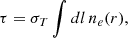
and if we ignore the internal motion, the kSZ effect is simplified to
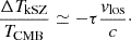
If we assume that there is no strong correlation between τ and |vlos|,

where  is the average optical depth of the cluster sample. The assumptions implied by this equation are tested on a cluster sample in hydro-simulation (Soergel et al. 2018).
2.2. Pairwise velocity
The pairwise velocity profile v12(r, z), depending on the 3D pair separation and redshift, is sensitive to the growth of cosmic structure. Linear theory shows

where fg is the cosmic growth rate, H is the Hubble parameter at the scale factor a, and ξ is the two-point correlation function. The halo correlation function ξh is related to ξ through the mass-averaged halo bias b, as the approximation ξh ≃ b2ξ.  is the averaged correlation function within a comoving radius, r (see Soergel et al. 2016 and Mueller et al. 2015 for detailed derivations).
2.3. Optical-cluster-selection bias
The optical-cluster-selection effect occurs when there is a conditional dependence between the richness residual Δlnλ and the residual of another observable ΔlnDobs at a given mass:

where λ is richness, defined as in the red-sequence matched-filter probabilistic percolation (redMaPPer) cluster finder (Rykoff et al. 2014). The cluster mass is denoted by M, and Dobs represents one of the cluster observables on which the bias might emerge, such as the kSZ effect or weak gravitational lensing. Δlnλ and ΔlnDobs represent the residuals of λ and the observable on the logarithmic space after removing their mass dependence, typically modeled by a power-law relation (see Wu et al. 2022 for a bivariate Gaussian model for lnλ and the lensing residual).
3. Simulations
To investigate the selection effect on kSZ signals, it is essential to accurately model the distribution of baryonic gas within the large-scale structures where halos are embedded. In this work, we used the hydrodynamical simulations of Magneticum1 (Dolag et al. 2025). Magneticum is a series of cosmological simulations that follow WMAP7 cosmology, including a comprehensive range of physical processes, such as a subgrid model of radiative cooling, a uniform time-dependent UV background, star formation and stellar feedback, growth of black holes, and feedback from active galactic nuclei (AGNs), which are essential for modeling the ICM (Hirschmann et al. 2014). The subgrid models are calibrated to reproduce the gas properties of clusters at z = 0. Remarkably, even without tuning to stellar properties, the simulations reproduce many stellar-based scaling relations (Dolag et al. 2025), while it could be challenging for cosmological simulations calibrated primarily to stellar properties to accurately model gas scaling relations and kinematic properties (Popesso et al. 2026; van de Sande et al. 2019). Moreover, Magneticum is able to reproduce the critical properties of SZ observations from Planck (Dolag et al. 2016, 2025). Therefore, the Magneticum simulations are particularly suitable for studying the ICM.
Several SZ products are constructed from Magneticum, such as light cones and full sky maps (Soergel et al. 2018; Dolag et al. 2016; Coulton et al. 2022). In this work, we analyzed a kSZ map along with the associated cluster and galaxy catalogs from a 5 × 5 deg2 light cone with a depth of z < 2.1, generated from Box2 of Magneticum by the SMAC code (Dolag et al. 2005)2. Box2 has a size of 352 h−1 cMpc and a mass of dark-matter particles of 6.9 × 10⁸ h−1 M⊙, which allowed us to resolve galaxies. The light cone is approximated by 27 redshift slices taken from random positions in the simulation box. This is because interpolating positions of gas particles between snapshots is challenging, especially for large hydrodynamical simulations, when the snapshots are relatively far from each other. The full depth kSZ map is the co-addition of the maps calculated from the redshift slices. The geometry of the z = 0.2 − 0.6 light cone is described in Table 1. The light cone provides multiwavelength mock data, including X-ray emission (Biffi et al. 2018), SZ Compton Y, the kSZ effect, and optical magnitudes (see Marini et al. 2024, 2025 for light-cone design). The stellar mass function in the simulation is complete down to 109.8 M⊙. The combination of comprehensive ICM physics and high resolution makes these simulations well suited for studying selection effects on kSZ measurements. We also verified that the mock sky coordinates from the flat light cone are sufficiently accurate for the pairwise kSZ analysis (see Appendix B). In addition, we used clusters from a 35 × 35 deg2 light cone (Soergel et al. 2018) to generate an empirical pairwise velocity template (see Appendix A). This larger light cone is based on Box0, which has moderate resolution and greater volume, making it suitable for capturing large-scale velocity statistics and resolving massive galaxy clusters.
Geometry and the redshift slices of the z = 0.2 − 0.6 region in the 5 × 5 deg2 light cone.
4. Methods
This section outlines the key steps in the investigation into optical-selection bias on kSZ observables across a wide range of galaxy-selection criteria. Section 4.1 details how galaxies were selected based on physical properties and how the cylindrical count method was applied to each set of the selection criteria to mimic the optical-cluster-selection process that assigns richness to each cluster. Section 4.2 describes how the observables – pairwise kSZ effect, pairwise velocity, and optical depth – were measured on the mock data products. Finally, Sect. 4.3 presents the estimation of selection bias by comparing signals of richness-selected halos with signals of equal mass distribution sets of halos selected purely by their mass.
4.1. Alternative richness
To mimic the optical-cluster-selection process, we implemented the method of cylindrical counts from Wu et al. (2022). The method defines a cylindrical region at the position of each cluster, with the depth of the cylinder corresponding to the photometric redshift uncertainty along the line of sight, and the aperture corresponding to the cluster size. The counts of galaxies in the cylinders serve as the alternative richness. The alternative richness accounts for the projection effect and avoids the color criteria of richness, which are challenging for simulations. The cylindrical counts have been shown to reproduce the selection effect that biases the weak lensing signal (Sunayama et al. 2020; Wu et al. 2022; Salcedo et al. 2024).
Here we describe the procedures for assigning alternative richness to each cluster. First, we selected subhalos in the light cone based on their stellar mass, average stellar age, and specific star formation rate (sSFR) to obtain a “bright” and “red” galaxy sample. These properties use all particles that are bound to each subhalo identified by the SUBFIND algorithm (Springel et al. 2001; Dolag et al. 2009). We define bright and red by the physical properties of all particles in each subhalo, because the goal is not to generate galaxy properties that are directly comparable with observations, but to explore a wide range of galaxy properties consistent with the M − λ relation of optical clusters. The stellar mass cut includes the redshift dependence of the characteristic magnitude, m*(z), of the Schechter luminosity function as redMaPPer (Rykoff et al. 2016). We adopted the m*(z) derived for the SDSS r-band from the model of Bruzual & Charlot (2003)3, with a (1 + z) evolution from the M/L ratio of elliptical galaxies, as considered in Saglia et al. (2010). The minimum value of each stellar mass cut, M★(z), is set at z = 0.65, and M★(z) increases as z decreases. The stellar mass function in the simulation is complete down to 109.8 M⊙.
Second, we selected the clusters at z = 0.2 − 0.6 to compare with DES results, with a minimum mass of log(M200m/h−1 M⊙) ≥ 12.1 to ensure the stellar masses of central galaxies were well resolved. For an accurate measurement of kSZ aperture photometry, clusters within 5 arcmin of the edge of the light-cone map were excluded. These criteria yielded a sample of 23 128 mock clusters. For simplicity, these mock catalogs assumed that the clusters to have the same locations and velocities as their central galaxies. In reality, among clusters, optically selected central galaxies, and gas, there could be offsets of positions and velocities, which is another effect to model in cosmological inferences (Calafut et al. 2017; Zhang et al. 2019; Orlowski-Scherer et al. 2021; Ding et al. 2024). This setup mimics the case of cross-matching optically selected central galaxies with spectroscopic redshift catalogs. Under this framework, the uncertainty in spectroscopic redshifts is negligible compared to other sources of uncertainty.
Third, we applied the cylindrical count pipeline to these two catalogs to assign richness to the clusters. We used R200 m as an approximation for the size of the cluster defined by redMaPPer,Rλ. The radius R200 m tends to be larger than Rλ for high-mass clusters and falls below it for low-mass clusters. Wu et al. (2022) showed that using an approximate aperture might increase the bias, as Rλ minimizes the scatter of X-ray luminosity at a fixed λ. If a galaxy is within the cylinders of multiple halos, it is considered to be a member of the most massive halo. The cylinder depth is defined as the maximum distance that can separate galaxies from the cluster center, and we used a range of 40–100 cMpc to account for photometric redshift uncertainty in recent surveys (the typical value is 50 cMpc for DES; see Soergel et al. 2016). Subsequently, we compared the best-fit M200 m − λ relation at λ ≥ 5 to the DES-Y1 relation (To et al. 2021a):

This comparison examines whether a set of galaxy-selection criteria is ruled out by observational data (Fig. 1).
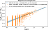 |
Fig. 1. M − λ relation of halos in the Magneticum 5 × 5 deg2 light cone, given a galaxy selection of M★ ≥ 109.8 M⊙, mean stellar age ≥ 4.2 Gyr, sSFR ≤ 10−15 yr−1, and cylindrical depth of 60 h−1 cMpc. The relation fit to λ ≥ 5 (dashed line) is consistent with DES-Y1 results within 1σ (To et al. 2021a, blue line and shaded region). |
4.2. Estimating the pairwise kSZ signal and its components
In this subsection, we investigate the pairwise kSZ observable and its components: pairwise velocity and optical depth. The measurement pipeline of pairwise kSZ effect and pairwise velocity is the updated version of iskay4 (Gallardo 2019; Gallardo et al. 2025). This tool has been utilized to analyze the pairwise kSZ effect on ACT data (Calafut et al. 2021). It can measure aperture photometry on the kSZ maps and measure the pairwise kSZ effect by the estimator of Ferreira et al. (1999),

where δTi is the kSZ temperature decrement for cluster i. Each cluster pair is separated by a comoving distance of r = |rij|=|ri − rj|, and cij is the geometry weighting regarding how the pair is aligned with the line of sight. In other words, cij = cos α, where α is the angle between the pairs and the line of sight. The uncertainties for pairwise kSZ profiles were estimated by bootstrapping the halo catalog 1000 times.
The aperture photometry measures the average temperature, TAP, within a radius of Rθ and subtracts the average temperature from an outer annulus at  . We used apertures of radius Rθ = 2.1 and 2.7 arcmin, motivated by the size of the light-cone halos with log M200m ≥ 13.40 h−1 M⊙ (corresponding to λ ≥ 5 in DES-Y1). The median R200 m for these halos at z = 0.2 − 0.6 is 2.52 arcmin. For Legacy Survey eROMaPPer clusters with λ ≥ 3.95 (which corresponds to λ ≥ 5 of DES-Y1, see Kluge et al. (2024)) at z = 0.01 − 1.0, the median Rλ is 2.19 arcmin. These sizes are also comparable to values used in previous studies based on luminous red galaxies (Calafut et al. 2021).
In typical pairwise kSZ measurements, a correction is applied to aperture photometry to remove potential redshift-dependent contamination from the foreground or large-scale motion (Hand et al. 2012). This correction subtracts a Gaussian-smoothed average  from fine redshift bins:

The Gaussian function G(zi, zj, σz) = exp[−(zi, zj)2/(2σz2)] is controlled by the redshift smoothing parameter σz. In our main analysis, we did not apply this redshift-evolution correction. This decision is based on the absence of significant redshift evolution in the kSZ temperatures measured over z = 0.2 − 0.6 in the light cone. The mock images do not include foreground contamination, so there is no evolution directly from them, nor indirectly from the correlation between them and the measurement process. In addition, due to the limited size of the light cone, we found that it is challenging to properly measure a global redshift evolution systematic without significantly removing the local motion signal. Applying this correction to the light cone could in itself introduce bias. Hence, we disabled this function when using iskay.
The optical depth of the cluster gas, τ, is a key property that can be inferred from kSZ measurements. When fitting pairwise velocity templates with a fixed cosmology to pairwise kSZ data, the fit amplitude corresponds to the average τ of the sample. To estimate the potential selection bias that may propagate from kSZ signals to τ, we estimated optical depth by fitting a simple linear regression line to ΔTkSZ − v in the fine mass bins. The regression line introduced a v2 weighting for each cluster, enhancing the signal compared to when directly averaging the ratio of ΔTkSZ to v. This method does not introduce bias, as the average peculiar velocity in each bin is expected to be zero and independent of mass. We verified that the mean velocities in the mass bins were consistent with zero and that the v2 weighting did not affect the main results. The uncertainty in τ for each mass bin was estimated by bootstrapping the halo catalog 1000 times.
4.3. Reconstruction of the unbiased signal
After obtaining the richness catalog, we studied the difference between the kSZ effect of a richness-selected sample and a reconstructed, unbiased signal. We used different approaches for pairwise observables and optical depth. The following describes the reconstruction of the pairwise kSZ effect and the pairwise velocities. A richness-selected sample was selected by richness cuts (λ ≥ 5 in this work) and was subjected to selection bias. A reconstructed signal PRecon(r) was mass selected, but each cluster was weighted according to its mass to reconstruct the underlying mass distribution of the richness-selected sample (Fig. 2):

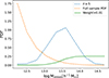 |
Fig. 2. Mass distribution of the clusters with λ ≥ 5, shown as probability distribution function (dashed blue line). The galaxy-selection criteria used here are the same as in Fig. 1. The dashed orange line represents the mass distribution of halos with log(M200m/h−1 M⊙) ≥ 12.1 in the light cone. The green line indicates the weight applied to reconstruct the unbiased signal, scaled by a factor of 0.01 for visual comparison. |
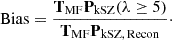
Namely, the weight, wi(Mi), represents the probability ratio that a cluster of a given mass will be selected by the richness cut to it being selected in the full halo catalog, given a specific galaxy selection. The bias value was estimated as the ratio between the richness-selected signal and the reconstructed unbiased signal (Fig. 3 illustrates an example):
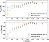 |
Fig. 3. Comparison of pairwise signal of the “richness-selected” and the “reconstructed” sample of clusters. The richness-selected sample is potentially subject to selection bias, where the reconstructed sample is mass-selected, unbiased, and weighted to match the mass probability distribution of the richness-selected sample. Using the same galaxy selection as in Fig. 1, the biases of pairwise kSZ effect, pairwise velocity, and optical depth are 1.10 ± 0.19, 1.01 ± 0.11, and 1.00 ± 0.08. |
We employed an optimized filter, TMF, while averaging the pairwise profile over the separation of pairs, to optimize the S/N. The filter was constructed from the empirical signal and error template from the Magneticum 35 × 35 deg2 light cone (see Appendix A). The uncertainty of the richness-selected or reconstructed signal was estimated by summing their covariance matrix with the filter:

This uncertainty was then propagated to the final bias ratio.
On the other hand, regarding the reconstruction of optical depth, since this parameter is estimated on individual clusters, there is an opportunity to further reduce the uncertainties. We followed the “weighting” method in Wu et al. (2022), splitting the sample into ten mass bins, calculating the average τ in each bin (see Sect. 4.2) and averaging the binned τ with the weighting of the mass distribution of the richness-selected sample (as Fig. 2).
5. Results and discussion
5.1. Selection bias
Here we elaborate on the main results. In Fig. 3, we present an example with a specific galaxy selection, stellar mass ≥ 109.8 M⊙, mean stellar age ≥ 4.2 Gyr, sSFR ≤ 10−15 yr−1, and the cylindrical depth = 60 h−1 cMpc. The richness-selected signal and the reconstructed signal (defined in Sect. 4.3) show no significant differences, and their ratio is consistent with unity. For both the pairwise kSZ effect and the pairwise velocities, no bias is observed at the current level of uncertainties. In the full analysis, this measurement was repeated on a broad range of galaxy-selection criteria that generate M − λ relations compatible with DES-Y1. The explorations of these selection criteria are shown in Fig. 4. Here the “min stellar mass” refers to the threshold applied at z = 0.65 (see Sect. 4.1 for the redshift evolution of the stellar mass cut). The grid displays the range of galaxy selections and cylindrical depths explored. Each combination produces a M − λ relation. The grids are color-coded according to the distribution of the M − λ relations that are compatible with DES-Y1. We examined both extremes of the galaxy bimodality by controlling the sSFR and mean stellar age. We used the most restrictive “red” criterion, which includes passive galaxies down to modest stellar mass, and the “bluest” criterion, which effectively removes the color criterion and only selects galaxies by stellar mass. The cylindrical depth and the stellar mass cut balance the “color” criteria, generating reasonable M − λ relations. The M − λ relations were compared with DES-Y1, on the full redshift range z = 0.2 − 0.6, and within four redshift bins of width 0.1.
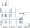 |
Fig. 4. Galaxy-selection criteria explored to examine if the M − λ relations are consistent with the DES-Y1 M − λ relation within 2 σ. The blue squares are color-coded by the distribution of the selection criteria that generate M − λ relations consistent with DES-Y1 across the full redshift range z = 0.2 − 0.6 and within each of the four redshift bins. The “min stellar mass” denotes the minimum value set at z = 0.65 for the redshift evolution of the stellar mass cut. |
Based on the alternative richness, for each galaxy selection we investigated the biases of pairwise kSZ signals, pairwise velocity, and optical depth (Fig. 5). For selections that yield M − λ relations consistent with DES-Y1 in the z = 0.2 − 0.6 range and within each of the four redshift bins, the biases are shown in the blue (DES 2σ) and orange (DES 1σ) violin plots. All these points are consistent with unity within 1σ. Figure 5 is based on a photometric aperture, Rθ = 2.7′, and Fig. 6 shows a similar result for Rθ = 2.1′, where the biases remain consistent with unity within 1.34σ. For Rθ = 2.7′, the result indicates that there is no significant bias on pairwise kSZ signals, pairwise velocity, or optical depth above the levels of 19%, 11%, and 9%, respectively. The median uncertainty levels across galaxy selections are 16%, 10%, and 8%, respectively.
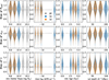 |
Fig. 5. Constraints on bias values based on a smoothing scale of Rθ = 2.7 arcmin and all galaxy-selection criteria explored (gray). The violin areas include both statistical errors and systematic errors within a set of proposed galaxy selections. Each bootstrap uncertainty is considered as a Gaussian kernel extended to 3σ. The widths of the violins are normalized to avoid overlapping. Bars indicate the range of bias values for each fixed parameter. The horizontal dashed lines mark the case of no bias (Bias = 1). The biases derived from M − λ relations consistent with DES-Y1 (To et al. 2021a) within 1σ (2σ) are shown in orange (blue). For Rθ = 2.7 arcmin, and with galaxy selections consistent with DES-Y1 both across the full redshift range and within each of the four redshift bins of width 0.1, the biases are consistent with unity within 1σ. No significant bias is observed. |
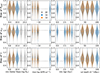 |
Fig. 6. Similar to Fig. 5 but for a smoothing scale of Rθ = 2.1 arcmin. For Rθ = 2.1 arcmin, and with galaxy selections consistent with DES-Y1 both across the full redshift range and within each of the four redshift bins of width 0.1, no significant bias is observed. The biases of the kSZ signal and velocities are consistent with unity within 1σ, and the biases of optical depth are within 1.34σ. |
5.2. Discussion
Figure 5 shows that the biases are consistent with one, indicating that no significant bias is observed in pairwise kSZ signals or their related properties. This contrasts with weak lensing, where the optical-selection bias is known to introduce considerable bias (Wu et al. 2022; Salcedo et al. 2024). Unlike weak lensing, where the signal scales linearly with mass, the projected kSZ signal does not follow a simple linear relation with optical depth or mass along the line of sight. The contribution from peculiar velocities of structures along the line of sight, combined with pairwise orientation and averaging, leads to a more complicated projection effect. We note that these findings apply specifically to the pairwise kSZ estimator and pairwise velocity. They may not directly generalize to other kSZ extraction approaches such as those based on velocity reconstruction. The uncertainty level of our test (∼19%) is comparable to the measurement uncertainties in previous pairwise kSZ detections using optically selected clusters, which have reached a significance level of ∼5σ. At this level of statistical precision, it is reasonable to expect that optical-selection bias does not play a dominant role. However, achieving tighter constraints will require larger simulation volumes with comparable resolution to improve statistical power, which will be essential for interpreting the higher significance pairwise kSZ measurements anticipated from upcoming datasets.
We assumed that τ and v have a negligible correlation when deriving the pairwise kSZ formula (Sect. 2.1). This assumption is verified by Soergel et al. (2018) on a cluster sample in Magneticum. However, we probed this relation down to a much lower mass. Given this assumption, the biases are expected to follow a similar relation, where the bias of τ will be equal to the ratio of bias of PkSZ and bias of v12. Our main result in Fig. 5 aligns with this assumption. Further investigation of this relationship and the τ − v correlation would require a larger simulation sample.
We also investigated the mass probability distribution functions in the richness bins [5, 10, 20, 30, 45, 60, inf]. We find that less restrictive stellar age or sSFR criteria result in wider distributions and heavier low-mass tails (Fig. 7). Compared with the distributions from Salcedo et al. (2024), which are based on a halo-occupation-distribution framework, the distributions in this work have fewer objects in the low-mass tail. Although the low-mass tail of the λ > 20 bins suffered from low number counts, fewer low-mass halos for a given richness implies less potential of selection bias. Future quantitative research for selection bias on the kSZ effect would require a larger simulation and a more sophisticated bias model to account for the M − λ relation in fine bins.
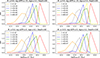 |
Fig. 7. Mass distributions in richness bins [5, 10, 20, 30, 45, 60, inf], given different galaxy-selection criteria that have M − λ consistent with DES-Y1. The upper left panel is based on a relatively restrictive passive selection, and the other panels are examples of less restrictive criteria. The less restrictive criteria make the distributions wider and generate stronger low-mass tails. |
Due to the limited size of the light cone, large-scale profiles (roughly beyond 200 cMpc) are highly uncertain. Furthermore, the Magneticum light cones are constructed by slices centered at random positions of the box, and neither the mass nor velocity is correlated across the slices. The slice sizes are comparable with the depth of the cylinder (see Table 1), which could reduce large-scale structure correlations with the clusters. However, these limitations affect both the richness-selected and the reconstructed samples in the same way. It would still be valuable to apply the same analysis on a larger light cone with a different construction.
The correction of redshift evolution (Sect. 4.2) is not applied in this work, as no significant redshift evolution is detected in the mock kSZ temperatures, and the limited size of the light cone makes the proper correction challenging. In future studies that include foregrounds, this correction will need to be enabled. We do not expect the redshift evolution correction to introduce additional selection bias, because it does not directly depend on richness. However, foregrounds such as residuals from the thermal SZ effect may correlate with richness and are worth testing. In principle, thermal SZ residuals primarily affect the most massive clusters, which are rare and less sensitive to the selection bias, so they are not expected to generate a significant additional bias.
6. Summary
The detection of the pairwise kSZ effect has now reached a significance level of more than 9σ. With the ongoing and upcoming large spectroscopic surveys, the constraining power of the kSZ effect on a scale of less than 50 cMpc is going to improve substantially. Robust modeling of systematics is essential to unlock this cosmological information.
In this work, we investigated the optical-cluster-selection bias on the pairwise kSZ effect, pairwise velocities, and optical depth. We applied the method of cylindrical counts to obtain reasonable M − λ relations in hydrodynamical simulations. We estimated the bias for λ ≥ 5 on clusters at z = 0.2 − 0.6 with M200m ≥ 1012.1 h−1 M⊙ over a wide range of galaxy-selection criteria. Within our uncertainty level, no significant bias was observed.
This result paves the way for upcoming pairwise kSZ measurements, with optical cluster samples powered by DESI spectroscopy, cross-matching with Atacama Cosmology Telescope (ACT, Coulton et al. 2024; Naess et al. 2025), Simons Observatory (Abitbol et al. 2025), and next-generation CMB efforts. Applying this framework to larger hydrodynamical simulations, ideally incorporating various feedback or cosmological models, and a light-cone structure complementary to Magneticum, would be highly valuable. For future work, a more sophisticated model would be required for a quantitative estimation, and investigating the bias of multi-observable probes – such as clustering and weak lensing – would provide deeper insights into the gas properties in large structures.
Acknowledgments
The authors would like to thank Luca Sala, Stephan Vladutescu-Zopp, Frederick Groth, Johannes Stoiber, and Rhea-Silvia Remus for valuable discussions and assistance with accessing Magneticum simulations and related tools. We also thank Andrés Salcedo and Tomomi Sunayama for insightful discussions on optical selection effects, as well as Justin Myles and Oliver Friedrich for helpful discussions. This work was funded by the Deutsche Forschungsgemeinschaft (DFG, German Research Foundation) under Germany’s Excellence Strategy – EXC-2094/2 – 390783311. IM acknowledges support from the European Research Council (ERC) under the European Union’s Horizon Europe research and innovation programme ERC CoG (Grant agreement No. 101045437). KD acknowledges support by the COMPLEX project from the European Research Council (ERC) under the European Union’s Horizon 2020 research and innovation program grant agreement ERC-2019-AdG 882679. The calculations for the Magneticum simulations were carried out at the Leibniz Supercomputer Center (LRZ) under the project pr83li.
References
- Abbott, T., Abdalla, F., Alarcon, A., et al. 2018, Phys. Rev. D, 98, 043526 [NASA ADS] [CrossRef] [Google Scholar]
- Abbott, T., Aguena, M., Alarcon, A., et al. 2020, Phys. Rev. D, 102, 023509 [NASA ADS] [CrossRef] [Google Scholar]
- Abitbol, M., Abril-Cabezas, I., Adachi, S., et al. 2025, J. Cosmol. Astropart. Phys., 2025, 034 [Google Scholar]
- Biffi, V., Dolag, K., & Merloni, A. 2018, MNRAS, 481, 2213 [Google Scholar]
- Bigwood, L., Amon, A., Schneider, A., et al. 2024, MNRAS, 534, 655 [NASA ADS] [CrossRef] [Google Scholar]
- Bruzual, G., & Charlot, S. 2003, MNRAS, 344, 1000 [NASA ADS] [CrossRef] [Google Scholar]
- Calafut, V., Bean, R., & Yu, B. 2017, Phys. Rev. D, 96, 123529 [Google Scholar]
- Calafut, V., Gallardo, P., Vavagiakis, E., et al. 2021, Phys. Rev. D, 104, 043502 [NASA ADS] [CrossRef] [Google Scholar]
- Chen, Z., Zhang, P., Yang, X., & Zheng, Y. 2022, MNRAS, 510, 5916 [NASA ADS] [CrossRef] [Google Scholar]
- Chisari, N. E., Mead, A. J., Joudaki, S., et al. 2019, Open J. Astrophys., 2, 1 [Google Scholar]
- Costanzi, M., Rozo, E., Rykoff, E. S., et al. 2018, MNRAS, 482, 490 [Google Scholar]
- Costanzi, M., Saro, A., Bocquet, S., et al. 2021, Phys. Rev. D, 103, 043522 [Google Scholar]
- Coulton, W., Feldman, S., Maamari, K., et al. 2022, MNRAS, 513, 2252 [NASA ADS] [CrossRef] [Google Scholar]
- Coulton, W., Madhavacheril, M. S., Duivenvoorden, A. J., et al. 2024, Phys. Rev. D, 109, 063530 [NASA ADS] [CrossRef] [Google Scholar]
- De Bernardis, F., Aiola, S., Vavagiakis, E., et al. 2017, J. Cosmol. Astropart. Phys., 2017, 008 [Google Scholar]
- DESI Collaboration (Abdul-Karim, M., et al.) 2025, arXiv e-prints [arXiv:2503.14745] [Google Scholar]
- Ding, J., Dalal, R., Sunayama, T., et al. 2024, MNRAS, 536, 572 [Google Scholar]
- Dolag, K., Hansen, F. K., Roncarelli, M., & Moscardini, L. 2005, MNRAS, 363, 29 [Google Scholar]
- Dolag, K., Borgani, S., Murante, G., & Springel, V. 2009, MNRAS, 399, 497 [Google Scholar]
- Dolag, K., Komatsu, E., & Sunyaev, R. 2016, MNRAS, 463, 1797 [Google Scholar]
- Dolag, K., Remus, R. S., Valenzuela, L. M., et al. 2025, A&A, accepted [arXiv:2504.01061] [Google Scholar]
- Ferreira, P. G., Juszkiewicz, R., Feldman, H. A., Davis, M., & Jaffe, A. H. 1999, ApJ, 515, L1 [NASA ADS] [CrossRef] [Google Scholar]
- Gallardo, P. A. 2019, https://doi.org/10.7298/kj4t-8e29 [Google Scholar]
- Gallardo, P. A., Gong, Y., Hadzhiyska, B., & Hsu, Y.-H. 2025, Res. Notes AAS, 9, 284 [Google Scholar]
- Gong, Y., Gallardo, P. A., Bean, R., et al. 2025, arXiv e-prints [arXiv:2511.23417] [Google Scholar]
- Hadzhiyska, B., Ferraro, S., Guachalla, B. R., et al. 2024, arXiv e-prints [arXiv:2407.07152] [Google Scholar]
- Hadzhiyska, B., Gong, Y., Hsu, Y., et al. 2025, arXiv e-prints [arXiv:2510.14135] [Google Scholar]
- Hand, N., Addison, G. E., Aubourg, E., et al. 2012, Phys. Rev. Lett., 109, 041101 [NASA ADS] [CrossRef] [Google Scholar]
- Hirschmann, M., Dolag, K., Saro, A., et al. 2014, MNRAS, 442, 2304 [Google Scholar]
- Kluge, M., Comparat, J., Liu, A., et al. 2024, A&A, 688, A210 [NASA ADS] [CrossRef] [EDP Sciences] [Google Scholar]
- Komatsu, E., Smith, K. M., Dunkley, J., et al. 2011, ApJS, 192, 18 [Google Scholar]
- Levi, M., Bebek, C., Beers, T., et al. 2013, arXiv e-prints [arXiv:1308.0847] [Google Scholar]
- Li, S., Zheng, Y., Chen, Z., Xu, H., & Yang, X. 2024, ApJS, 271, 30 [Google Scholar]
- Marini, I., Popesso, P., Lamer, G., et al. 2024, A&A, 689, A7 [NASA ADS] [CrossRef] [EDP Sciences] [Google Scholar]
- Marini, I., Popesso, P., Dolag, K., et al. 2025, A&A, 694, A207 [NASA ADS] [CrossRef] [EDP Sciences] [Google Scholar]
- McCarthy, I. G., Amon, A., Schaye, J., et al. 2024, arXiv e-prints [arXiv:2410.19905] [Google Scholar]
- Mueller, E.-M., de Bernardis, F., Bean, R., & Niemack, M. 2014, ApJ, 808, 47 [Google Scholar]
- Mueller, E.-M., de Bernardis, F., Bean, R., & Niemack, M. D. 2015, Phys. Rev. D, 92, 063501 [NASA ADS] [CrossRef] [Google Scholar]
- Myles, J., Gruen, D., Mantz, A. B., et al. 2021, MNRAS, 505, 33 [NASA ADS] [CrossRef] [Google Scholar]
- Naess, S., Guan, Y., Duivenvoorden, A. J., et al. 2025, arXiv e-prints [arXiv:2503.14451] [Google Scholar]
- Orlowski-Scherer, J., Di Mascolo, L., Bhandarkar, T., et al. 2021, A&A, 653, A135 [NASA ADS] [CrossRef] [EDP Sciences] [Google Scholar]
- Osato, K., Nishimichi, T., Oguri, M., Takada, M., & Okumura, T. 2018, MNRAS, 477, 2141 [NASA ADS] [CrossRef] [Google Scholar]
- Planck Collaboration XXXVII. 2015, A&A, 586, A140 [Google Scholar]
- Popesso, P., Biviano, A., Marini, I., et al. 2026, A&A, 707, A362 [NASA ADS] [CrossRef] [EDP Sciences] [Google Scholar]
- Rykoff, E. S., Rozo, E., Busha, M. T., et al. 2014, ApJ, 785, 104 [Google Scholar]
- Rykoff, E. S., Rozo, E., Hollowood, D., et al. 2016, ApJS, 224, 1 [NASA ADS] [CrossRef] [Google Scholar]
- Saglia, R. P., Sánchez-Blázquez, P., Bender, R., et al. 2010, A&A, 524, A6 [NASA ADS] [CrossRef] [EDP Sciences] [Google Scholar]
- Salcedo, A. N., Wu, H.-Y., Rozo, E., et al. 2024, Phys. Rev. Lett., 133, 221002 [Google Scholar]
- Schiappucci, E., Bianchini, F., Aguena, M., et al. 2023, Phys. Rev. D, 107, 042004 [Google Scholar]
- Soergel, B., Flender, S., Story, K. T., et al. 2016, MNRAS, 461, 3172 [Google Scholar]
- Soergel, B., Saro, A., Giannantonio, T., Efstathiou, G., & Dolag, K. 2018, MNRAS, 478, 5320 [NASA ADS] [CrossRef] [Google Scholar]
- Springel, V., White, S. D., Tormen, G., & Kauffmann, G. 2001, MNRAS, 328, 726 [NASA ADS] [CrossRef] [Google Scholar]
- Sugiyama, N. S., Okumura, T., & Spergel, D. N. 2018, MNRAS, 475, 3764 [NASA ADS] [CrossRef] [Google Scholar]
- Sunayama, T., Park, Y., Takada, M., et al. 2020, MNRAS, 496, 4468 [CrossRef] [Google Scholar]
- Sunyaev, R. A., & Zeldovich, Y. B. 1980, MNRAS, 190, 413 [NASA ADS] [CrossRef] [Google Scholar]
- To, C., Krause, E., Rozo, E., et al. 2021a, Phys. Rev. Lett., 126, 141301 [NASA ADS] [CrossRef] [Google Scholar]
- To, C. H., Krause, E., Rozo, E., et al. 2021b, MNRAS, 502, 4093 [NASA ADS] [CrossRef] [Google Scholar]
- To, C.-H., Pandey, S., Krause, E., et al. 2024, J. Cosmol. Astropart. Phys., 2024, 037 [Google Scholar]
- van de Sande, J., Lagos, C. D. P., Welker, C., et al. 2019, MNRAS, 484, 869 [NASA ADS] [CrossRef] [Google Scholar]
- Wu, H.-Y., Costanzi, M., To, C.-H., et al. 2022, MNRAS, 515, 4471 [CrossRef] [Google Scholar]
- Zhang, Y., Jeltema, T., Hollowood, D. L., et al. 2019, MNRAS, 487, 2578 [NASA ADS] [CrossRef] [Google Scholar]
- Zhang, Z., Wu, H.-Y., Zhang, Y., et al. 2022, MNRAS, 523, 1994 [Google Scholar]
- Zubeldia, I., Rotti, A., Chluba, J., & Battye, R. 2021, MNRAS, 507, 4852 [NASA ADS] [CrossRef] [Google Scholar]
Appendix A: Matched filter
We employed the matched filter approach to combine the pairwise kSZ signal over a range of separations in a way that optimizes the S/N. Assume that the data vector d is a linear combination of a signal template sm(r), amplitude a0, and noise nm,

We can find a linear transform that maximizes the S/N of our a0 estimation (see e.g. Zubeldia et al. 2021 for the detailed derivation), as

where Cm is the noise covariance matrix model. The optimized S/N is given as

We obtained the signal template sm and the covariance template Cm empirically from the Magneticum 35 × 35 deg2 light cone (Soergel et al. 2018). We fitted a smoothed broken power law function to the pairwise velocity profile of the z = 0.2 − 0.6 clusters up to 150 cMpc and adopted it as sm. The potential redshift evolution was corrected (see Sect. 4.2). The smoothing parameter Δ was set to 1:
![Mathematical equation: $$ f(x) = A \left( \frac{x}{x_b} \right)^{-\alpha _1} \left\{ \frac{1}{2} \left[ 1 + \left( \frac{x}{x_b} \right)^{1/\Delta } \right] \right\} ^{(\alpha _1 - \alpha _2) \Delta } \,. $$](/articles/aa/full_html/2026/08/aa55553-25/aa55553-25-eq23.gif)
There were 23, 177 clusters selected with Mvir ≥ 1013.5 h−1 M⊙, which is similar to the mass cut corresponding to λ ≥ 5, which is M200m ≥ 1013.4h−1 M⊙. Although this selection differs slightly from our main sample due to the simulation resolution, the template is only used to obtain a higher S/N while summing up the profile, and the main result is not sensitive to the shape of the template.
The error model was obtained by fitting a log-linear relation, to the logarithm of the standard deviation of the 4000 times bootstrap realizations of the pairwise kSZ curve. We assumed the covariance is highly diagonal, which is reasonable within 150 cMpc (Fig. A.1). The bias result is based on the ratio between two signals, so the normalization of the filter is irrelevant – only the shape matters. If we ignore the normalization denominator, the numerator T ≈ smTCm−1 weights the signal as shown in Fig. A.2. The shape of the template captures two critical features: there is little signal beyond 150 cMpc, and the uncertainties are large within 20 cMpc.
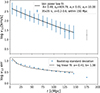 |
Fig. A.1. Signal and covariance templates for the optimized filter, obtained from the pairwise velocity of clusters in the 35 × 35 deg2 light cone. The fitting parameters for the empirical templates are presented in the plot. The x-axis indicates the comoving separation of the cluster pairs. Templates are fitted up to 150 cMpc. |
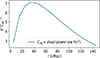 |
Fig. A.2. Illustration of the shape of the numerator of the filter |

Appendix B: Light-cone sky coordinates approximation
This section verifies that the mock sky coordinates in the light-cone catalog are sufficiently accurate for the pairwise kSZ analysis. The light-cone images are constructed by co-adding images from flat simulation slices (see Sect. 3). The mock galaxy positions in (R.A., Dec.) are derived from pixel coordinates, using the ratio between the image angular size and the number of pixels. For the 5×5 deg2 image, the angular pixel size is
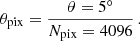
Here Npix is the number of pixels in the mock image. Since the pairwise estimation involves computing large separations between galaxies, and we apply the observational pipeline to mock products, it is important to verify the accuracy of this approximation.
We performed a test to compare distances computed using the exact Cartesian positions with those obtained from the approximate mock sky coordinates. The exact distance calculation takes the Cartesian (X, Y, Z) positions of each mock cluster, where X, Y are obtained from the light-cone geometry and Z from the Hubble redshift of each halo. These positions were converted to sky coordinates (R.A., Dec.) in degrees and radial comoving distance D in h−1cMpc



These coordinates are only used for distance calculation, and do not affect the sample selection. The photometry pipeline is not affected by this approximation, since it operates on Plate-Carrée projection that is consistent with the mock sky coordinates.
The test was performed on the 23, 128 mock clusters selected in Sect. 4.1. These clusters were located at redshift z = 0.2 − 0.6 and had a minimum mass of log (M200m/h−1M⊙)≥12.1. The comparison is shown in Fig. B.1, where the pairwise velocities obtained from the approximated and exact sky coordinates agree well within the uncertainties estimated by bootstrapping the cluster catalog 1000 times. Therefore, the impact of the sky coordinate approximation is negligible.
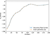 |
Fig. B.1. Comparison between the exact distance calculation and the approximate sky coordinates used in the mock catalog. Pairwise velocities computed from exact Cartesian (X, Y, Z) coordinates (orange dotted line), and from the mock Plate-Carrée coordinates (blue solid line) are fully consistent. Uncertainties are estimated by bootstrapping the cluster catalog 1000 times. |
All Tables
Geometry and the redshift slices of the z = 0.2 − 0.6 region in the 5 × 5 deg2 light cone.
All Figures
|
Fig. 1. M − λ relation of halos in the Magneticum 5 × 5 deg2 light cone, given a galaxy selection of M★ ≥ 109.8 M⊙, mean stellar age ≥ 4.2 Gyr, sSFR ≤ 10−15 yr−1, and cylindrical depth of 60 h−1 cMpc. The relation fit to λ ≥ 5 (dashed line) is consistent with DES-Y1 results within 1σ (To et al. 2021a, blue line and shaded region). |
| In the text | |
|
Fig. 2. Mass distribution of the clusters with λ ≥ 5, shown as probability distribution function (dashed blue line). The galaxy-selection criteria used here are the same as in Fig. 1. The dashed orange line represents the mass distribution of halos with log(M200m/h−1 M⊙) ≥ 12.1 in the light cone. The green line indicates the weight applied to reconstruct the unbiased signal, scaled by a factor of 0.01 for visual comparison. |
| In the text | |
|
Fig. 3. Comparison of pairwise signal of the “richness-selected” and the “reconstructed” sample of clusters. The richness-selected sample is potentially subject to selection bias, where the reconstructed sample is mass-selected, unbiased, and weighted to match the mass probability distribution of the richness-selected sample. Using the same galaxy selection as in Fig. 1, the biases of pairwise kSZ effect, pairwise velocity, and optical depth are 1.10 ± 0.19, 1.01 ± 0.11, and 1.00 ± 0.08. |
| In the text | |
|
Fig. 4. Galaxy-selection criteria explored to examine if the M − λ relations are consistent with the DES-Y1 M − λ relation within 2 σ. The blue squares are color-coded by the distribution of the selection criteria that generate M − λ relations consistent with DES-Y1 across the full redshift range z = 0.2 − 0.6 and within each of the four redshift bins. The “min stellar mass” denotes the minimum value set at z = 0.65 for the redshift evolution of the stellar mass cut. |
| In the text | |
|
Fig. 5. Constraints on bias values based on a smoothing scale of Rθ = 2.7 arcmin and all galaxy-selection criteria explored (gray). The violin areas include both statistical errors and systematic errors within a set of proposed galaxy selections. Each bootstrap uncertainty is considered as a Gaussian kernel extended to 3σ. The widths of the violins are normalized to avoid overlapping. Bars indicate the range of bias values for each fixed parameter. The horizontal dashed lines mark the case of no bias (Bias = 1). The biases derived from M − λ relations consistent with DES-Y1 (To et al. 2021a) within 1σ (2σ) are shown in orange (blue). For Rθ = 2.7 arcmin, and with galaxy selections consistent with DES-Y1 both across the full redshift range and within each of the four redshift bins of width 0.1, the biases are consistent with unity within 1σ. No significant bias is observed. |
| In the text | |
|
Fig. 6. Similar to Fig. 5 but for a smoothing scale of Rθ = 2.1 arcmin. For Rθ = 2.1 arcmin, and with galaxy selections consistent with DES-Y1 both across the full redshift range and within each of the four redshift bins of width 0.1, no significant bias is observed. The biases of the kSZ signal and velocities are consistent with unity within 1σ, and the biases of optical depth are within 1.34σ. |
| In the text | |
|
Fig. 7. Mass distributions in richness bins [5, 10, 20, 30, 45, 60, inf], given different galaxy-selection criteria that have M − λ consistent with DES-Y1. The upper left panel is based on a relatively restrictive passive selection, and the other panels are examples of less restrictive criteria. The less restrictive criteria make the distributions wider and generate stronger low-mass tails. |
| In the text | |
|
Fig. A.1. Signal and covariance templates for the optimized filter, obtained from the pairwise velocity of clusters in the 35 × 35 deg2 light cone. The fitting parameters for the empirical templates are presented in the plot. The x-axis indicates the comoving separation of the cluster pairs. Templates are fitted up to 150 cMpc. |
| In the text | |
|
Fig. A.2. Illustration of the shape of the numerator of the filter |
| In the text | |
|
Fig. B.1. Comparison between the exact distance calculation and the approximate sky coordinates used in the mock catalog. Pairwise velocities computed from exact Cartesian (X, Y, Z) coordinates (orange dotted line), and from the mock Plate-Carrée coordinates (blue solid line) are fully consistent. Uncertainties are estimated by bootstrapping the cluster catalog 1000 times. |
| In the text | |
Current usage metrics show cumulative count of Article Views (full-text article views including HTML views, PDF and ePub downloads, according to the available data) and Abstracts Views on Vision4Press platform.
Data correspond to usage on the plateform after 2015. The current usage metrics is available 48-96 hours after online publication and is updated daily on week days.
Initial download of the metrics may take a while.