A deep study of the spiral galaxy W2246f

Evelyn J. Johnston; Sorya Lambert; Aparna Nair; Alejandra Z. Lugo-Aranda; Manuel Aravena; Roberto J. Assef; Tanio Diaz Santos; Román Fernández Aranda; Hyunsung D. Jun; Guodong Li; Mai Liao; Devika Shobhana; Chao-Wei Tsai

doi:10.1051/0004-6361/202660281

Home

All issues

Volume 711 (July 2026)

A&A, 711 (2026) A194

Full HTML

Open Access

Issue		A&A Volume 711, July 2026


Article Number		A194
Number of page(s)		14
Section		Extragalactic astronomy
DOI		https://doi.org/10.1051/0004-6361/202660281
Published online		14 July 2026

A&A, 711, A194 (2026)

A deep study of the spiral galaxy W2246f

Evelyn J. Johnston¹^★, Sorya Lambert¹, Aparna Nair², Alejandra Z. Lugo-Aranda³, Manuel Aravena¹^,4, Roberto J. Assef¹, Tanio Diaz Santos⁵^,6, Román Fernández Aranda⁷, Hyunsung D. Jun⁸, Guodong Li⁹, Mai Liao¹, Devika Shobhana¹ and Chao-Wei Tsai¹⁰^,11^,12

¹ Instituto de Estudios Astrofísicos, Facultad de Ingeniería y Ciencias, Universidad Diego Portales, Av. Ejército Libertador 441, Santiago, Chile
² Instituto de Astronomía y Ciencias Planetarias, Universidad de Atacama, Avenida Copayapu 485, 1530000, Copiapó, Chile
³ Universidad Nacional Autónoma de México, Instituto de Astronomía, AP 106, Ensenada, 22800, BC, Mexico
⁴ Millenium Nucleus for Galaxies (MINGAL)
⁵ Institute of Astrophysics, Foundation for Research and Technology Hellas (FORTH), Heraklion, 70013, Greece
⁶ School of Sciences, European University Cyprus, Diogenes Street, Engomi, 1516, Nicosia, Cyprus
⁷ Centro de Astrobiología (CAB), CSIC-INTA, Carretera de Ajalvir km 4, Torrejón de Ardoz, 28850, Madrid, Spain
⁸ Department of Physics, Northwestern College, 101 7th St SW, Orange City, IA, 51041, USA
⁹ Kavli Institute for Astronomy and Astrophysics, Peking University, Beijing, 100871, People’s Republic of China
¹⁰ National Astronomical Observatories, Chinese Academy of Sciences, 20A Datun Road, Beijing, 100101, China
¹¹ Institute for Frontiers in Astronomy and Astrophysics, Beijing Normal University, Beijing, 102206, China
¹² School of Astronomy and Space Science, University of Chinese Academy of Sciences, Beijing, 100049, China

^★ Corresponding author: This email address is being protected from spambots. You need JavaScript enabled to view it.

Received: 7 April 2026
Accepted: 27 May 2026

Abstract

Aims. In this era of large surveys and statistical studies of galaxies, the beauty in the details of individual galaxies is often lost. In this paper we present a deep study of the spiral galaxy W2246f with MUSE, exploring the spatially resolved stellar and ionised gas properties to understand how it formed and evolved over time. The unusually deep observations of this galaxy with MUSE give us a rare opportunity to study this phenomenon with a better spatial resolution than can normally be achieved with the current IFU surveys of galaxies at a similar redshift (z ∼ 0.09).

Methods. We analyse the stellar and gas kinematics, as well as the spatially resolved stellar populations and gas properties, including gas metallicity and the dominant ionisation sources. The derived properties include the stellar mass, radial profiles of luminosity- and mass-weighted mean ages and metallicities, and ionised gas characteristics such as E(B − V), Hα extinction, dust-corrected Hα flux, oxygen abundance using the O3N2 calibrator, Hα luminosity, and the Hα-based star formation rate.

Results. Analysis of the stellar populations revealed a negative metallicity gradient, and the mass-weighted ages showed uniformly flat ages across the disc while the luminosity-weighted ages show a negative gradient. We find that the gas metallicity and star formation rate density also drop in the central region of the galaxy where the older luminosity-weighted stellar populations are found. Analysis of the WHAN and WHaD diagrams reveal that in fact the central region is retired, while the rest of the disc is star-forming.

Conclusions. We conclude that W2246f is a nice example of a central low-ionisation emission-line region (cLIER) galaxy, where the central kpc is dominated by old, metal-poor stars with little star formation. The cLIER emission is primarily powered by hot evolved stars, while the rest of the disc displays ongoing star formation. These findings are consistent with a scenario of inside-out quenching.

Key words: galaxies: general / galaxies: ISM / galaxies: individual: W2246f / galaxies: spiral / galaxies: stellar content

© The Authors 2026

Open Access article, published by EDP Sciences, under the terms of the Creative Commons Attribution License (https://creativecommons.org/licenses/by/4.0), which permits unrestricted use, distribution, and reproduction in any medium, provided the original work is properly cited.

This article is published in open access under the Subscribe to Open model. This email address is being protected from spambots. You need JavaScript enabled to view it. to support open access publication.

1. Introduction

As astronomical research makes increasing use of large surveys and statistical samples, there is still a lot to learn from studying the fine details of individual galaxies to better understand these processes. Spiral galaxies are home to the ongoing recycling of gas in the Universe, with clouds of gas collapsing to trigger the formation of new stars, while the death of older stars injects new metals, such as oxygen, nitrogen, and sulphur, back into the interstellar medium (ISM) where they can enrich the next generation of stars to be created (Matteucci & Francois 1989). Over the last decade, integral field unit (IFU) spectroscopy has revolutionised the study of the structural components of all types of galaxies, including spirals, providing spatially resolved spectroscopic information across their entire extent. This information has shed new light on how galaxies have formed and evolved compared to what could be learnt previously from multi-object or long-slit spectroscopy alone.

For example, long-slit spectroscopy found clear gradients in the stellar ages and metallicities across galaxy discs, where generally the older and more metal-rich stellar populations lie in inner regions of galaxies, suggesting an inside-out growth over time (Tissera et al. 2016; Goddard et al. 2017; Peterken et al. 2020; Lara-López et al. 2022; Pessa et al. 2023). However, IFU spectroscopy has revealed that these gradients are not smooth, but instead show bumps or flatter regions, particularly close to spiral arms and bars. Such features indicate that these structures are driving the migration of gas and stars, meaning that the older stars may now lie very far from where they were formed (Di Matteo et al. 2013; Ruiz-Lara et al. 2017). Thus, it has become clear that spiral galaxies continue to evolve and change throughout their lifetimes.

With IFU spectroscopy we can map out the stellar and gas kinematics of spiral galaxies. While in most cases these kinematics maps will show smooth variations across the discs, perturbations can indicate recent interactions or mergers. For example, it is thought that the presence of kinematically decoupled cores (KDCs) and counter-rotating discs indicate the remnant of a smaller galaxy that has merged with the spiral galaxy. During this merger, the infalling galaxy has lost the majority of its mass, and the material from its core has settled into the centre of the galaxy and maintains some of the angular momentum of the progenitor galaxy (e.g. Krajnović et al. 2015; Johnston et al. 2018; Nedelchev et al. 2019). The relative sizes of the two kinematic components and the degree of asymmetry can also help us understand the properties of the two progenitor galaxies and the conditions under which they interacted or merged (Bao et al. 2022). Furthermore, the kinematics maps can also reveal structures such as nuclear discs (e.g. Medling et al. 2014; Gadotti et al. 2020) and active galactic nucleus (AGN) jets (e.g. Venturi et al. 2017) that are significantly harder to detect and characterise with long-slit spectra alone.

Another benefit of IFU spectroscopy is that one can map out the gas properties across a spiral galaxy in order to understand the different ionisation sources that dominate in the different regions (Sánchez 2020). Generally in spiral galaxies, the majority of the disc is dominated by star formation, but in the centres of these galaxies an AGN might be present (e.g. Belfiore et al. 2015, 2016; Fensch et al. 2016; Ma et al. 2021). By mapping out the ratios of different emission lines it is possible to understand the extent and strength of these AGNs. For example, Belfiore et al. (2016) studied a sample of low-ionisation nuclear emission-line region galaxies (LINERs) from the MaNGA survey and found that the LINER emission is often not restricted to only the central region of the galaxy, but in some cases can be detected across large parts of the disc. He named these galaxies LIERs to reflect this broader distribution of low ionisation emission.

Along with new instruments with large fields of view and high spatial resolution, such as the Multi-Unit Spectroscopic Explorer (MUSE; Bacon et al. 2010) and the Visible Integral-field Replicable Unit Spectrograph (VIRUS; Hill et al. 2021), came new IFU surveys to observe large samples of galaxies in a more statistical way. For example, the SDSS-IV Mapping of Nearby Galaxies at APO (MaNGA: Bundy et al. 2015) survey observed ∼10 000 galaxies within z < 0.15 out to 1.5 − 2.5 R_e, the Calar Alto Legacy Integral Field Area (CALIFA; Sánchez et al. 2016) survey achieved similar coverage for > 600 galaxies out to z ∼ 0.16, and the Sydney-AAO Multi-object Integral field spectrograph (SAMI; Croom et al. 2012; Bryant et al. 2015) observed a further ∼3000 galaxies out to z ∼ 0.1. Together, these three surveys shed new light on galaxy morphology and evolution, and paved the way for smaller, more specific surveys, such as the MUSE Atlas of DISCS (MAD; Erroz-Ferrer et al. 2019), the Time Inference with MUSE in Extragalactic Rings (TIMER; Gadotti et al. 2019), and the PHANGS-MUSE survey (Emsellem et al. 2022). However, one weakness of many of these surveys is that in order to resolve the features within these galaxies, one must observe relatively nearby galaxies that often are larger than the field of view (FOV) of the instrument. As a result, many of these surveys focus on the properties in the inner regions of the galaxies, and lose the information from the outskirts, where perturbations due to recent interactions and mergers are likely to be seen for longer (Borlaff et al. 2014; Eliche-Moral et al. 2018; Martínez-Delgado et al. 2025). One new IFU survey that will achieve full coverage of nearby galaxies is the SDSS-V Local Volume Mapper (LVM; Drory et al. 2024), with a wide FOV of ∼30′, but this coverage comes with the sacrifice of the spatial resolution (∼36″ fibers).

As a result, despite the abundance of large surveys and statistical studies of galaxies, there is still room for detailed studies of individual galaxies, especially where particularly deep or high-resolution data are available. This paper outlines one such study of W2246f, also known as Leda 1044720, a spiral galaxy located at RA 22^h46^m08^s.3 and Dec −05° 26′24.5″ (J2000) that happens to lie in the foreground of a deep (∼20 hours exposure time) MUSE datacube studied in Shobhana et al (in prep.). The datacube is centred on WISE J224607.6–052634.9 (W2246–0526), a hot, dust-obscured galaxy (also known as a Hot DOG; Wu et al. 2012) at redshift z ∼ 4.6 (Díaz-Santos et al. 2018), and the focus of the work by Shobhana et al (in prep.) is to study the environment of this galaxy. W2246f was previously studied by Fan et al. (2018) in the context of understanding its contamination in their studies of W2246–0526, and they retrieved a photometric redshift for W2246f of z_ph = 0.047 from the Sloan Digital Sky Survey SkyServer¹. The datacube used in this study covers the entire galaxy with a high spatial resolution (∼0.2 arcsec pixel⁻¹), with the deep exposure time ensuring a good signal even in the outermost regions. In this paper we carry out analysis of the stellar and gas kinematics, the stellar populations, and the gas properties to better understand the nature of this galaxy.

The paper is laid out as follows: Section 2 describes the observations and data reduction; Section 3 describes the visual morphology of the galaxy; Section 4 explores the stellar and gas kinematics; Section 5 studies the stellar properties; Section 6 gives an overview of the gas properties; and Section 7 presents our summary and conclusions. Throughout this paper we assume a Hubble constant of H₀ = 70 km s⁻¹ Mpc⁻¹ (Lelli et al. 2010), which corresponds to a projected angular scale of 1.83 kpc arcsec⁻¹ and a distance of 377 Mpc based on the line-of-sight velocity of the galaxy described in Section 4.

2. Observations and data reduction

The data used in this study were observed with MUSE on the Very Large Telescope (VLT). MUSE is an optical integral-field spectrograph with a FOV of 1′×1′, a spatial resolution of 0.2″/pixel, and a spectral resolving power ranging from R ≃ 1770 at 4800 Å to R ≃ 3590 at 9300 Å. The data were observed between July and September 2022 as part of programme IDs 106.21F0.001 (PI Diaz-Santos) and 109.2393.001 (PI Assef). The main target for these programmes was W2246–0526 (Tsai et al. 2015; Díaz-Santos et al. 2016, 2018; Tsai et al. 2018), the most luminous obscured quasar in the Universe at redshift z ∼ 4.6 (Fan et al. 2018). The spiral galaxy studied in this work happens to lie along a similar line of sight and appears in the upper left quadrant of the FOV of the MUSE datacube. Due to the faintness of the main target, the MUSE datacube is very deep, consisting of 104 exposures each with an exposure time of 675 s, resulting in a total exposure time of 19.5 hours for a single pointing. The data were observed in Wide Field Mode with AO using the nominal wavelength range (WFM-AO-N), and the average seeing was measured to be ∼0.65″ on the final combined datacube.

A full description of the data reduction is given in Shobhana et al (in prep.), but in summary the data were reduced using the ESO MUSE pipeline (Weilbacher et al. 2012) in the ESO Recipe Execution Tool (EsoRex) environment (ESO CPL Development Team 2015). The reduction was carried out using the standard procedure, which included creating master bias, flat field, and wavelength calibrations for each CCD and for each night of observations, which were then applied to the raw science and standard-star observations as part of the pre-processing steps. The data for each night were then flux-calibrated using the standard stars for each night, and the sky background was measured from the science data after masking out W2246f and the extended emission from W2246–0526. As part of the sky subtraction process, we also applied the self-calibration step within EsoRex, which applies an autocalibration on the slice-level to smooth the sky background across the entire FOV. Finally, the data were stacked, and the Zurich Atmosphere Purge code (ZAP, Soto et al. 2016) was used to remove any residual sky contamination from the final datacube.

The white-light image of the galaxy, created from the MUSE datacube, is shown in the left panel of Fig. 1, alongside two colour images. The middle image was created using the white-light image centred on Hα in red, [O III] in green, and the stellar continuum in blue, whereas the rightmost image shows the continuum-subtracted Hα, [O III] and [N II] emission in green, blue, and red, respectively. One can also see that there is a smaller galaxy on the upper edge of the datacube that shows gas emission, particularly in [O III], at a similar redshift as W2246f. A foreground star also lies on the eastern edge of W2246f, and this region was masked out during the analysis to prevent contamination.

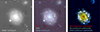Fig. 1.

Images of W2246f and its companion galaxy to the north-west, extracted from the MUSE datacube. On the left is the white light image showing the stellar continuum. In the middle is an RGB image with the Hα emission in red, the [O III] emission in green and the stellar continuum in blue. In this image the Hα and [O III] maps have not been continuum subtracted. On the right is a continuum-subtracted image showing the [N II] λ6584 emission in red, the Hα emission in green, and the [O III] emission in blue. The images are oriented with north up and east to the left, and a scale bar is shown in the stellar continuum image for reference, where 5″ corresponds to ∼9.15 kpc.

3. Morphology

The first step in the analysis of W2246f was to consider its morphology and physical properties. As can be seen in Fig. 1, W2246f is a flocculent spiral galaxy of class Sc, based on a visual inspection of the data used in this study. We used the MUSE datacube to create images of the galaxy in the g and r bands, and modelled the surface brightness profile using GALFIT (Peng et al. 2002, 2010). The best fit was found with a two-component model representing a bulge and disc. It was found that the bulge dominates the light within a radius of ∼2″ (∼3.66 kpc) in all filters, and the galaxy has a mean bulge-to-total (B/T) light ratio of 0.25, indicating that it is disc-dominated.

We used the magnitudes of the bulge and disc from the GALFIT fits to calculate the total magnitude of the galaxy in each filter, and used the g and r band magnitudes to estimate the stellar mass using

$\begin{matrix} log(M_{*} {[M}_{⊙}]) = 0.673 \times M_{g} - 1.108 \times M_{r} + 0.996 \end{matrix}$ $Mathematical equation: $$ \begin{aligned} \text{ log(} M_* \text{[M}_\odot \text{])}=0.673\times M_g - 1.108 \times M_r + 0.996 \end{aligned} $$$ (1)

(Ebrová et al. 2025), where M_g and M_r are the absolute magnitudes in the g and r band filters, respectively. This calculation gave a total stellar mass of 4.6 ± 1.1 × 10¹⁰ M_⊙. The uncertainties in this measurement come from both the uncertainties in the equation and from the magnitudes given by GALFIT. Häußler et al. (2007) and Häußler et al. (2013) found that the uncertainties derived by GALFIT are often substantially underestimated, since it assumes that any residual flux is due purely to Poisson noise, and does not take into account the effect of a poorly fitted model or other irregular structures, such as spiral arms. Nedkova et al. (2021) found that for modelling two components, such as the bulge and disc, the uncertainties from GALFIT are of the order of 2 − 2.5 times too small, so we followed their guide of multiplying the GALFIT magnitude errors by a factor of 3 in order to be conservative in the mass estimate above. This stellar mass is higher than the mass derived by Fan et al. (2018) of $1.1 \begin{matrix} + 0.5 \\ - 0.2 \end{matrix} \times 10^{10}$ $Mathematical equation: $ 1.1 \substack{+0.5 \\ -0.2} \times 10^{10} $$ M_⊙, which could be due to factors such as the methods used to measure the magnitudes (2-component fits with GALFIT in this paper versus aperture photometry in Fan et al. 2018), the number of filters used to derive the magnitudes and therefore the mass (2 versus 18), and the methods used to derive the mass (Equation (1) versus spectral energy distribution (SED) fitting).

4. Stellar and gas kinematics

The next step was to determine the connection between W2246f and the smaller galaxy to the north by calculating their redshifts using their line of sight velocities. The data were spatially binned using the PowerBin software of Cappellari (2025), which applies a 2D adaptive spatial binning to obtain binned spectra with more or less the same ‘capacity’, in this case signal-to-noise ratio (S/N). For W2246f a S/N of 50 in the stellar continuum was selected, and for the fainter companion the data were binned using S/Ns of 20, 30, and 40 in order to confirm any detections made at lower S/N.

Having binned the spectra, the kinematics (line-of-sight velocity, v, and velocity dispersion, σ) for each bin were measured using the penalised pixel fitting (pPXF) code of Cappellari (2023). For W2246f the h₃ and h₄ coefficients were also measured. The stellar spectra were modelled using template spectra from the E-MILES stellar library (Vazdekis et al. 2016), which were created using the Padova isochrones and Salpeter IMF and cover a wide range of well-defined ages (0.6 < Age < 15.8 Gyrs) and metallicities (−1.71 < [M/H] < +0.22). Simultaneously, the gas emission lines (Hγ, He IIλ4687, Hβ, [O III] λ5007, He I λ5876, [O I] λ6300, Hα, [N II] λ6583, [S II] λ6716, [S II] λ6731]) were modelled using Gaussian emission line spectra. All the templates for the stellar and gas components were convolved with line-of-sight velocity distributions and velocity dispersions to obtain a model spectrum that best fits each binned galaxy spectrum, and additive polynomials of order 6 were applied to model the flux calibration of the continuum and reduce template mismatch. The fits were run twice, first with the Balmer and forbidden lines constrained to have the same kinematics, and the second time they were modelled as two distinct kinematical components. However, no significant difference was found in their kinematics when they were modelled separately, and so the plots shown in this paper present the results from the fit using a single gas component that includes all the Balmer and forbidden lines.

The maps for the stellar and gas kinematics for W2246f are shown in Fig. 2. These measurements were derived through fits to the spectra over the optical region (4700 < λ < 8100 Å, which corresponds to a rest frame wavelength range of 4303 < λ < 7409 Å), but no significant differences were seen when modelling shorter ranges of the stellar continuum or individual emission lines. It can be seen that both the stars and the gas display a uniform and consistent velocity map, indicating that the galaxy has not undergone any significant mergers or interactions in the last ∼0.5 − 1 billion years (Hung et al. 2016; Davis & Bureau 2016) that would disrupt the stars and gas and leave a signature in their kinematics.

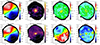Fig. 2.

Maps of the stellar (top) and gas (bottom) kinematics, showing from left to right the line of sight velocities, velocity dispersions and h₃ and h₄ coefficients for W2246f. The contours represent the flux in the white light image for reference, and the axes labels represent the distance in arcseconds from the centre of the galaxy.

Both the gas and the stars show a peak in the velocity dispersion at the centre of the galaxy, with the stellar σ being slightly higher at the centre of the galaxy. One interesting thing to note is the band of slightly higher gas σ across the minor axis of the galaxy. This feature is consistent with the ‘B distribution of σ’ that was described by Pilyugin et al. (2021). They found that ∼13% of the MaNGA galaxies in their sample showed this band of higher σ across the minor axis of the galaxies. They theorised that this feature could appear in cases where the gas velocity dispersion is asymmetric, i.e. where the radial component of the gas velocity dispersion (i.e. along the line of sight) is greater than the azimuthal (orbiting the galaxy plane) and vertical (perpendicular to the galaxy plane) components. However, they found no evidence that this feature is related to the presence of an AGN. Another study by Marconcini et al. (2025) also found evidence of the B distribution in the active galaxy NGC 424, lying perpendicular to the high-velocity outflow. They theorised that this outflow may enhance the B distribution of σ by injecting energy into the host disc and perturbing the ambient material. However, a full understanding of the origin of this effect is still missing in the literature, and so we report it here as simply another galaxy in which the feature is detected.

The h₃ and h₄ Gauss-Hermite coefficients are also interesting. These coefficients represent the skewness and kurtosis, respectively, and represent the non-Gaussianity in the shapes of the absorption and emission lines. The stellar h₃ map shows a clear anti-correlation with the velocity map in the inner region of the galaxy with some areas of slightly enhanced h₄, which together likely represents the presence of two kinematic components – a cold, rapidly rotating disc and a hotter, slower component, such as a bulge. The gas h₃ also shows a very strong anti-correlation with the gas velocity, while the h₄ coefficient is generally very negative with a few regions of stronger positive values. These maps indicate that the gas is orbiting as a dynamically cold disc, but is more structurally complex than the stellar disc, likely due to turbulence induced along the spiral arms or star-forming regions. These results, particularly the anti-correlation between velocity and h₃, are consistent with the predictions of Naab et al. (2014) for galaxies that built up their mass through in situ star formation along with gas-rich mergers, and with Class 3 and 4 galaxies (fast rotators with a strong disc component) observed by van de Sande et al. (2017) in the SAMI survey.

The kinematics analysis outlined above was then repeated for the neighbouring galaxy. While the stellar continuum was too faint to obtain reliable spatially resolved kinematics measurements, it was possible to combine the spectra from the whole galaxy into a single spectrum to derive the mean stellar kinematics. The gas emission, on the other hand, was bright enough to derive kinematics maps for a S/N of 20. These maps are shown in Fig. 3. One can see a smooth velocity curve, indicating that this galaxy is rotating along a similar axis as W2246f. There are also two peaks in the velocity dispersion plot. While these peaks are only small compared to the velocity dispersion of the rest of the galaxy, they appear close to two regions of strong [O III] emission shown in Fig. 1, and were also seen when the datacube was binned to different S/Ns. They are also both offset from the centre of the galaxy, which perhaps rules out ionisation from an AGN. Thus, it is likely that these regions reflect areas of enhanced star formation (Green et al. 2010, 2014; Yu et al. 2019).

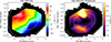Fig. 3.

Maps showing the stellar line-of-sight velocities (left) and velocity dispersions (right) for the neighbouring galaxy to W2246f. The contours represent the flux in the white light image for reference.

Having measured the kinematics of both galaxies, we then calculated their redshifts and physical separation. W2246f was found to lie at a redshift of 0.09223 ± 0.00009, while the satellite has a redshift of 0.09200 ± 0.00009, which correspond to distances of 377.1 ± 0.3 Mpc and 376.1 ± 0.3 Mpc, respectively. The two galaxies have a separation on sky of ∼19.5″, which corresponds to a physical separation on sky of ∼35.5 kpc at the distance of W2246f. Taking into account their distances from us, we found that they have a physical separation of 1.0 ± 0.7 Mpc. However, it should be noted that this distance is an upper limit on their separation assuming that their line-of-sight velocities correspond directly to their distance to us and relative to one another, i.e. assuming zero proper motion between them.

In the literature, galaxies are considered to have a close companion (i.e. to be a pair) or to be interacting when their separation is less than 30 kpc (e.g. Michel-Dansac et al. 2008; Ellison et al. 2008; Robaina et al. 2009; Patton et al. 2011, 2024), in some cases up to 100 − 150 kpc (e.g. Nikolic et al. 2004; Li et al. 2008; Casteels et al. 2013; Shah et al. 2022; Byrne-Mamahit et al. 2024). Thus, with a separation of ∼1 Mpc, it is unlikely that the two galaxies are interacting or form a gravitationally bound pair. However, it is possible that they reside in the same group or cluster environment, where other members of the group lie outside of the FOV of the data (e.g. Chernin et al. 2000). Thus, for the rest of this paper we focus our analysis on W2246f.

5. Stellar populations

The next step in the analysis was to study the stellar populations across W2246f in order to understand the star formation history of the galaxy. This analysis was carried out through a study of the mass- and luminosity-weighted stellar populations. Since the youngest stars are the hottest and brightest stars in the galaxy, they dominate the light even though they only account for a small fraction of the mass. Thus, the luminosity-weighted ages and metallicities give an insight into the most recent episode of star formation, since this phase created these hot, bright stars. However, the majority of the mass of a galaxy lies in older, fainter, and less massive stars, and so a study of the mass-weighted stellar populations gives a better overview as to how the mass of the galaxy built up over time, and is less biased towards more recent episodes of star formation that dominate the light. Together, the luminosity and mass-weighted stellar populations allow us to build up a clearer picture of the star formation history across the galaxy.

For this analysis we took the binned spectra from the kinematics analysis and used pPXF to derive estimates of the mass- and luminosity-weighted ages and metallicities. The first step was to correct for the galactic extinction. Since this galaxy has a very high galactic latitude, the galactic foreground reddening is relatively small, with a value of E(B − V) = 0.0292 calculated from Schlafly & Finkbeiner (2011) using the IRSA Galactic dust reddening tool². We then applied the Fitzpatrick (1999) extinction curve to calculate the extinction in magnitudes, A_λ, which was then applied to the binned spectra.

For the fits with pPXF, we used the same templates and wavelength range as for the kinematics measurements, described in Section 4. The fits were convolved with multiplicative polynomials of order 6, 8, and 10 to account for the shape of the continuum, reducing the sensitivity to dust reddening, and omitting the requirement of a reddening curve. Upon comparing the results derived using each order polynomial, it was found that the ages and metallicities start to converge to consistent values for multiplicative polynomials of orders 8 and 10, whereas those derived using an order of 6 tended to significantly overestimate ages and metallicities, which is consistent with a scenario where the continuum is underfitted (Cappellari 2017, 2023). Therefore, we selected a multiplicative polynomial of order 8 for the analysis presented in this paper, since it provides the optimal fit without underfitting the continuum or risking oversmoothing the spectrum such that any broad absorption features are included in the fit to the continuum. The fits were also carried out using regularisation, which works to create a smoothed variation in the weights of the templates with similar ages and metallicities. To determine the level of regularisation, we took a spectrum from the centre of the galaxy with a high S/N and carried out an unregularised fit to measure the χ² value. The noise spectrum was then scaled until χ²/N_d.o.f. = 1, where N_d.o.f. is the number of degrees of freedom in the fit, which corresponds to the number of unmasked pixels in the input spectrum. We then repeated the fit to the spectrum using this scaled noise spectrum and increasing value for the regularisation parameter until the χ² of the fit increased by $Δ χ^{2} = \sqrt{2 \times N_{d . o . f .}}$ $Mathematical equation: $ \Delta\chi^2 = \sqrt{2\times N_{d.o.f.}} $$ . This value represents the limit between a smooth fit that still reflects the star formation history of the galaxy and one that has been smoothed excessively. It should be noted at this point that this smoothed fit may not reflect the true star formation history of that part of the galaxy, which is likely to vary over shorter timescales than the models allow, but instead acts to reduce the age-metallicity degeneracy between spectra, allowing for a more consistent comparison of systematic trends in their star formation histories. Having determined the best regularisation value for this spectrum, this value was then applied to the fit to the remaining spectra of the galaxy. An example of these fits to two of the binned spectra are presented in Fig. 4, showing the fit to a spectrum close to the centre of the galaxy and another one further out in the disc.

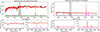Fig. 4.

Example fits with pPXF to two spectra from the galaxy. On the left is a spectrum taken from close to the centre of the galaxy where the A/N for the Hα line is weakest, and on the right is a spectrum from the disc. The top plots show the fits over the entire wavelength range, and the plots below show a zoom-in on the Hβ and [O III] emission lines on the left and the Hα and [N II] emission lines on the right. In all plots, the black line represents the binned spectrum from the galaxy, the red and magenta lines are the best fits to the stars and gas, respectively, the orange line shows the combined best fit, and the green points are the residuals. Note that the emission lines and residuals have been offset to higher values to better display the fits.

The weights for each template spectrum in each fit were then used to calculate the mean luminosity and mass-weighted ages and metallicities for each binned spectrum using

$\begin{matrix} log(Age) = \frac{\sum ω_{i} {log(Age}_{template, i})}{\sum ω_{i}} \end{matrix}$ $Mathematical equation: $$ \begin{aligned} \text{ log(Age)}=\frac{\sum \omega _{i} \text{ log(Age}_{\text{template},i})}{\sum \omega _{i}} \end{aligned} $$$ (2)

and

$\begin{matrix} [M/H] = \frac{\sum ω_{i} {[M/H]}_{template, i}}{\sum ω_{i}}, \end{matrix}$ $Mathematical equation: $$ \begin{aligned} \text{[M/H]}=\frac{\sum \omega _{i} \text{[M/H]}_{\text{template},i}}{\sum \omega _{i}} ,\end{aligned} $$$ (3)

respectively, where ω_i represents the weight of the i^th template (i.e. the value by which the i^th stellar template is multiplied to best fit the galaxy spectrum), and [M/H]_{template, i} and Age_{template, i} are the metallicity and age of the i^th template, respectively. The results are shown in Fig. 5, with the ages on the top row and metallicities on the bottom row. On the left are the radial plots, with the mass- and luminosity-weighted measurements in red and blue, respectively, and on the right are the radial maps for these properties.

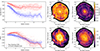Fig. 5.

Overview of the mass- and luminosity-weighted ages (top) and metallicities (bottom). On the left are radial plots for these properties, with the red and blue points representing the measurements from each binned spectrum for the mass- and luminosity-weighted stellar populations, respectively. The solid lines represent the rolling average for each dataset, and the shaded areas show the 1σ variation in this average. On the right are the mass and luminosity-weighted stellar population maps, where the contours reflect the variation in the white light image created from the datacube.

Considering first the stellar ages, one can see that the mass-weighted ages are relatively flat across the galaxy, with slightly older stars at the centre. This result is consistent with a galaxy that has undergone relatively constant star formation across the whole disc over most of its life, with an older bulge at the centre that formed early and has undergone little star formation since then. Due to the relatively old ages and small radial differences at radii larger than ∼2″, where the disc dominates the light, it is not possible to say whether the disc of the galaxy has formed inside-out or outside-in. On the other hand, the luminosity-weighted ages show a clear negative gradient in the inner region, within a radius of ∼2 − 3″ where the ages drop from around 6 − 7 billion years at the core to 1.5 billion years, and then a flatter gradient in the rest of the disc. This result is consistent with a galaxy that has ongoing star formation throughout the disc, and where the star formation in the inner region has been truncated somehow, leading to older stars there. From the light profile fitting described in Section 3, we found that the bulge dominates the light at the centre of the galaxy, and the disc starts to dominate the light at a radius of ∼2″. This radius corresponds to approximately to the second contour from the centre of the galaxy shown in Fig. 2 and in subsequent figures. Therefore, it is possible that this trend in the luminosity-weighted ages reflects the dominance of the older bulge stellar populations at the very centre of the galaxy, and with the increasing proportion of disc light as the radius increases.

However, despite the contribution of the bulge, the disc itself could also show a slight negative age gradient. Many studies have found negative age gradients in spiral discs. For example, Goddard et al. (2017) and Pessa et al. (2023) found negative luminosity-weighted age gradients in a large sample of MaNGA and PHANGS-MUSE galaxies, respectively. Pessa et al. (2023) also found negative mass-weighted age gradients in their galaxies, which they attributed to inside-out formation, where the inner regions of the galaxy formed earlier than the outskirts.

The flat mass- and luminosity-weighted age gradients across the disc may indicate one of several growth scenarios. For example, they may reflect that the galaxy did not build up its mass through a slow inside-out growth mechanism since this process would typically produce a strong negative age gradient. Or, if such a process did occur, it happened long enough ago that the age gradient has been smoothed out due to continuous star formation and is now difficult to detect. Sánchez-Blázquez et al. (2014) also found flatter mass-weighted age gradients across the discs of their sample of CALIFA galaxies, with typical ages of around ∼10 Gyrs, suggesting that another factor could be radial mixing over the lifetime of the galaxy.

Moving onto the stellar metallicity, it can be seen that both the mass- and luminosity-weighted metallicity curves show a negative gradient. Interestingly, the mass-weighted metallicities increase slightly from the centre out to a radius of ∼2″ before decreasing again towards the edges of the galaxy. This drop at the very centre aligns with the region of older luminosity-weighted stellar populations, and is consistent with the scenario in which the star formation in that region has been truncated, reducing the chemical enrichment there relative to other parts of the disc that have ongoing star formation.

The decrease in stellar metallicity from a radius of ∼2″ towards the outskirts of the galaxy could reflect longer star formation in the inner disc than the outer disc, which would lead to higher chemical enrichment of the ISM through supernovae or stellar winds (e.g. Lara-López et al. 2022), or perhaps accretion of pristine material into the outskirts of the disc (e.g. Aragon-Calvo & Szalay 2013; Aragon Calvo et al. 2019; Egorova et al. 2026), reducing the metallicity there. In the outermost regions of the galaxy, the luminosity-weighted metallicities can be seen to be slightly higher in general than the mass-weighted metallicities. This region coincides with the younger luminosity-weighted ages, and is consistent with more recent or more active star formation in that region producing younger stars and higher chemical enrichment. Negative metallicity gradients, and also negative age gradients, are common in spiral galaxies (e.g. Lian et al. 2018; Parikh et al. 2021; Pessa et al. 2023), with steeper gradients seen in more massive and late type galaxies similar to W2246f (Sánchez-Blázquez et al. 2014; Goddard et al. 2017), and are often attributed to inside-out formation or growth of the galaxy disc (Tissera et al. 2016; Breda et al. 2020).

6. Gas properties

The stellar populations, particularly the stellar metallicity, tell us about the long-term state of the ISM enrichment over the last 1 − 10 billion years, in particular about the conditions within the galaxy at the time that the stars were created (e.g. Gibson 1997). However, the ISM is continuously enriched through stellar evolution processes such as Type II supernova explosions, stellar winds from massive and asymptotic giant branch (AGB) stars, and ongoing star formation. As a result, to understand the current chemical enrichment of the ISM, one must instead examine the properties of the ionized gas, which trace enrichment processes operating on relatively short timescales of 10 − 100 million years (Mannucci et al. 2005; Scannapieco & Bildsten 2005; Sullivan et al. 2006; Matteucci et al. 2009; Brandt et al. 2010; Maoz et al. 2011; Maoz & Mannucci 2012).

6.1. BPT diagrams

The first step in analysing the gas properties was to identify the main source of ionisation across the galaxy, such as star formation or AGNs, using variations of the BPT diagram of Baldwin et al. (1981). For each binned spectrum, the emission lines were modelled alongside the stellar continuum with pPXF, which corrected the emission line fluxes for any absorption lines present at the same wavelengths. The emission line ratios were then calculated and plotted onto the BPT diagram shown in the top left panel of Fig. 6. The mean uncertainty for the spectra in each region of the BPT diagram (star-forming, composite, and AGN) are shown above the legend, having been calculated from the fits with PPXF.

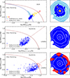Fig. 6.

BPT diagram for W2246f at the top along with the [S II] (middle) and [O I] diagnostic diagrams on the left. The brown curves represent the maximum starburst line of Kewley et al. (2001), the dashed brown lines represent the separation between Seyferts and LINERs from Kewley et al. (2006), and the blue curve in the top plot represents the pure star-forming line of Kauffmann et al. (2003). The error bar above the legend represents the median uncertainties in the line ratios. The uncertainties in the BPT diagram at the top have been separated according to the binned spectra that lie in the star-forming, composite, and AGN regions of the diagram, and use the same colour scheme. The maps on the right demonstrate the distribution of the bins in each region of the diagnostic diagrams over the galaxy.

The top plot in Fig. 6 shows the BPT diagram for [N II]/Hα and [O III]/Hβ, which is sensitive to metallicity and ionisation state. The data here displays the characteristic ‘Y’ shape seen in galaxies with both star formation and an AGN present. To better understand this BPT diagram, the BPT map of the galaxy is shown on the right of Fig. 6, where the colours represent the bins in different parts of the BPT diagram on the left. The majority of the disc lies on the star-forming branch, which has been separated into the upper and lower parts in the BPT diagram (coloured light and dark blue, respectively). The inner part of the disc lies on the lower part of this branch in the BPT diagram, while the outer part of the disc lies towards the top of the star-forming branch. The shape of the star-forming branch in the BPT diagram is driven by many factors, such as the gas-phase metallicity, the stellar mass, star formation rate (SFR), the hardness of the ionising radiation, the ionisation parameter, and the relative abundances of N/O versus O/H, to name but a few. These effects do not scale linearly with each other, which produces the curved shape for the star-forming branch, such as can be seen in Fig. 6. However, a study by Curti et al. (2022) found that, to a first order, the shape of the star-forming branch of the BPT diagram primarily traces the gas-phase metallicity, from higher metallicities at the bottom of the branch to lower metallicities and more younger O-class stars towards the upper part of the branch. Thus, in this galaxy, the BPT diagram is reflecting higher gas phase metallicities in the inner disc and lower metallicities in the outer disc. This trend is consistent with the stellar metallicity trend seen in Fig. 5, and with the distribution of Hα and [O III] in Fig. 1, where the [O III] is strongest in the outer part of the disc. [O III] is a high ionisation line, and its distribution can suggest the presence of hot stars in the inner regions of the HII regions, since these young massive stars tend to form in regions with lower-metallicity gas.

The central region of the galaxy lies to the right of the star-forming branch and towards the LINER (red) and composite (yellow) regions of the BPT diagram. Normally, this trend would indicate the presence of an AGN at the centre of the galaxy. However, when comparing to the right panel of Fig. 1 one can see that this central region of the galaxy contains very strong [N II] emission but very weak Hα emission, which might be enhancing the [N II]/Hα line ratios in that part of the galaxy. Similarly, it can be seen that the uncertainties for the data points in this region are larger than in the star-forming branch, potentially also indicating that at least one of the line strengths is getting weaker and that the uncertainty is proportionally larger.

Two variations of the BPT diagram are regularly used to help further refine the dominant ionising sources across galaxies. These diagrams use the [S II]/Hα and [O I]/Hα line ratios against [O III]/Hβ (Veilleux & Osterbrock 1987; Kewley et al. 2001, 2006), hereafter referred to as the [S II] and [O I] diagnostic diagrams. The [S II] diagnostic diagram is used to better distinguish between Seyferts and LINERS, but in the diagram shown in the middle panel of Fig. 6 it can be seen that all the line ratios from across the galaxy lie within the star-forming region of this diagram. The [O I] diagnostic diagram, on the other hand, is useful for identifying ionisation from shocks, since it is more sensitive to hard ionising radiation and partially ionised zones. Typically, if regions of a galaxy have been ionised by shocks, they overlap with the LINER region in the [O I] diagnostic diagram. However, it can be seen in Fig. 6 that the central region of this galaxy again lies in the star-forming region of the diagnostic diagram, indicating that if shocks are present there, their effect is negligible.

In general, although the classical BPT diagram is widely used, it has important limitations. The ‘composite’ region between star-forming and AGN-dominated zones (Kauffmann et al. 2003; Kewley et al. 2001) can include low-luminosity or metal-poor AGNs, supernova remnants, and even purely star-forming regions (e.g. Agostino & Salim 2019; Cid Fernandes et al. 2021). Recent studies have also found that galaxies at high redshift, such as the little red dots observed with JWST, appear to lie in the composite and star-forming regions, likely due to their lower metallicity (e.g. Nakajima & Maiolino 2022; Kocevski et al. 2023; Übler et al. 2023; Harikane et al. 2023; Maiolino et al. 2024). Finally, evolved ionising sources, such as post-AGB stars and hot low-mass evolved stars (HOLMESs), can mimic AGN-like line ratios despite weaker emission, and shocks – both fast and slow – can also produce similar ratios depending on gas conditions and shock velocity (e.g. Binette et al. 1994; Dopita & Sutherland 1996; Flores-Fajardo et al. 2011; López-Cobá et al. 2020). These ambiguities make interpreting BPT diagrams challenging.

6.2. WHAN and WHaD diagrams

In response to the need for a better identification of ionising sources, we used hybrid diagnostic diagrams that incorporate not only flux intensities but also additional parameters, such as the estimated equivalent width (Cid Fernandes et al. 2011) and velocity dispersion (Sánchez et al. 2024). Stasińska et al. (2008) found that the LINER region of the BPT diagram also contains galaxies that have stopped forming stars, and which are instead ionised by the HOLMESs, such as hot post-AGB stars and white dwarfs, contained in them. In these regions, the emission line strengths would be weaker than those produced by star formation or AGNs, but the line ratios would still cover a wide range of values, overlapping with those typically seen in star-forming regions or AGNs. They called these galaxies ‘retired galaxies’ to differentiate them from passive galaxies, which contain no or very low or undetectable levels of emission. Later studies with IFU data found that these line ratios are not only seen in retired galaxies, but also retired regions within galaxies (e.g. Singh et al. 2013; Belfiore et al. 2017; Lacerda et al. 2018). However, with the BPT diagram on its own, it is difficult to identify these galaxies or regions.

In order to better distinguish between retired galaxies or regions in galaxies and LINERS, Cid Fernandes et al. (2011) proposed the W_Hα versus [N II]/Hα (WHAN) diagram. The WHAN diagram uses the equivalent width of Hα, W_Hα, to separate these two regimes, since star-forming galaxies and AGNs would be expected to have stronger Hα emission lines than retired galaxies. The first step towards plotting the WHAN diagram was to correct the Hα flux for dust extinction before calculating the equivalent width. For this step we used the Balmer decrement to measure the level of dust attenuation across W2246f. The theoretical value of the Balmer decrement is 2.86 for case-B recombination (Osterbrock 1989; Calzetti et al. 2000) for a fixed electron temperature of T_e = 10 000 K and density of n_e = 100 cm⁻³ (Hummer & Storey 1987). Therefore, any deviation from this theoretical value can be considered an effect of dust extinction (Groves et al. 2012).

We first calculated the foreground dust reddening along the line of sight using

$\begin{matrix} E (B - V) = \frac{2.5}{k (H β) - k (H α)} \times log (\frac{F {(H α)}_{o} / F {(H β)}_{o}}{2.86}) \end{matrix}$ $Mathematical equation: $$ \begin{aligned} E(B-V) = \frac{2.5}{k(H\beta ) - k(H\alpha )} \times \text{ log}\Bigg (\frac{F(H\alpha )_o/F(H\beta )_o}{2.86}\Bigg ) \end{aligned} $$$ (4)

(Domínguez et al. 2013), where the extinction coefficients k(Hβ) and k(Hα) come from the reddening curve described in Cardelli et al. (1989), and F(Hα)_o and F(Hβ)_o are the observed Hα and Hβ fluxes. We then calculated the extinction at Hα, A_α, using

$\begin{matrix} A_{H α} = k (H α) \times E (B - V) \end{matrix}$ $Mathematical equation: $$ \begin{aligned} A_{\mathrm{H}\alpha } = k(H\alpha ) \times E(B-V) \end{aligned} $$$ (5)

(Calzetti et al. 2000). The maps for the dust reddening and extinction are given in Fig. 7, where it can be seen that the galaxy contains a moderate amount of dust that is mainly concentrated in the inner region of the disc.

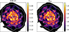Fig. 7.

Reddening (left) and extinction (right) maps of W2246f.

Having calculated the dust extinction, we could then correct the observed Hα flux and derive the intrinsic Hα flux, F(Hα)_i, using

$\begin{matrix} F {(H α)}_{i} = F {(H α)}_{o} \times 10^{0.4 A_{H α}} . \end{matrix}$ $Mathematical equation: $$ \begin{aligned} F(H\alpha )_{i} = F(H\alpha )_{o} \times 10^{0.4\ A_{\mathrm{H}\alpha }}. \end{aligned} $$$ (6)

Finally, having corrected the Hα flux for dust extinction, we derived the W_Hα and plotted the WHAN diagram shown in the top panel of Fig. 8. Since weak emission lines can be hard to model accurately, especially if their amplitude approaches the level of noise in the spectrum, their fluxes and consequently the W_Hα can be affected. For example, the fluxes of weak emission lines in low-S/N spectra could be underestimated, leading to a misclassification of that region as retired. In order to prevent this situation, the amplitude-to-noise ratio (A/N) for the Hα line was measured in the fit to each binned spectrum in order to identify potential cases where the Hα emission line could be hidden in the noise. In general we found very high A/Ns for all the binned spectra, with the minimum A/N being ∼21, and the fit to this spectrum is shown in the left panel of Fig. 4. As a result, we did not need to mask any points in the WHAN diagram due to unreliable measurements of the emission line flux.

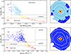Fig. 8.

WHAN (top) and WHaD (bottom) diagrams for W2246f on the left and the corresponding maps on the right. The grey lines demonstrate the regions of each diagram that are dominated by different ionisation sources, such as star formation (SF), Seyferts (sAGN), LINERS (wAGN), and HOLMES in retired regions of the galaxy. The error bars on the left show the mean uncertainties for the points in each region of the diagram, where the points in the star-forming and Seyferts regions of the WHAN diagram have been combined to give a single error. The colours in the plots and the maps reflect which part of the WHAN and WHaD diagram those bins lie in to better show their spatial distribution across the galaxy.

The colours of the data points in the top panel of Fig. 8 correspond to which region of the WHAN diagram they lie in – star-forming (SF) in dark blue, Seyferts in light blue, LINERS in yellow, and retired in orange – and the map on the right of the figure shows the distribution of these regions across the galaxy. One can see that the centre of the galaxy has relatively low W_Hα (< 3 Å), putting this region in the retired region instead of the LINER region. This region coincides with the area marked as a LINER and composite region from the BPT diagram in Fig. 6 based on the [N II]/Hα ratio, and the presence of post-AGB stars is consistent with the old luminosity-weighted stellar populations seen in this region in Fig. 5.

However, this diagram puts the majority of the disc into the LINERS and Seyferts region of the WHAN diagram, which is unlikely to be real. The vertical line separating the star-forming and active galaxies at log [N II]/Hα = −0.4 corresponds to the optimal transposition of the Stasińska et al. (2008) BPT-based SF/AGN division, which is designed to differentiate sources where star formation provides all ionising photons from those where a harder ionising spectrum is required. It can be seen in the bottom panel of Fig. 6 that the star-forming branch spans both the star-forming and composite regions of the BPT diagram as well. The horizontal position of the star-forming branch can be affected by several factors. For example, galaxies with higher metallicities or higher N/O ratios will typically display higher [N II]/Hα ratios, pushing them into the composite region on the BPT diagram (e.g. Pérez-Montero & Contini 2009; Belfiore et al. 2017; Curti et al. 2022). This scenario is likely to be the case for W2246f in the BPT and WHAN diagrams.

More recently, Sánchez et al. (2024) proposed WHaD diagram of W_Hαversus the velocity dispersion of Hα, σ_Hα, to better differentiate between the different ionising sources present in a galaxy. In this case, they used a single line, Hα for the analysis, making this diagram useful in cases where the other key emission lines are not covered or where the S/N is too low in those lines. The WHaD diagram for W2246f is given in the bottom of Fig. 8 along with the spatial distribution of the points. It can be seen that, again, the central region of the galaxy lies in the retired section of the diagram, and the majority of the disc lies in the star-forming part of the diagram.

Based on these results, it appears that the BPT diagram over-interpreted the hardness of the ionising radiation field in W2246f. While the [N II]/Hα BPT diagram suggested that the centre of this galaxy contains a LINER, through the analysis of the WHAN and WHaD diagrams it has become clear that in that region of the galaxy the emission is weak and consistent with an old stellar population, rather than with an AGN. Our results are consistent with the category of central low-ionisation emission-line region (cLIER) galaxies proposed by Belfiore et al. (2016), which are described as galaxies in which the LIER emission is resolved but concentrated in the central regions, while ionisation from star formation dominates at larger galactocentric distances.

6.3. Gas metallicity

The shape of the star-forming branch in the BPT diagram is defined by various factors, such as the SFR and gas metallicity. In order to study more deeply the relationship between gas metallicity and the position along the star-forming branch on the BPT diagram, we calculated the gas metallicity using the O3N2 indicator:

$\begin{matrix} O3N2 = log (\frac{[NII] 6584 / H α}{[OIII] 5007 / H β}) . \end{matrix}$ $Mathematical equation: $$ \begin{aligned} \text{ O3N2} = \text{ log} \Bigg (\frac{[\text{ NII}]6584/\text{ H}\alpha }{[\text{ OIII}]5007/\text{ H}\beta } \Bigg ). \end{aligned} $$$ (7)

We then calculated the gas phase metallicity using

$\begin{matrix} 12 + log(O/H) = 8.73 - 0.32 \times O3N2 \end{matrix}$ $Mathematical equation: $$ \begin{aligned} 12+\text{ log(O/H)}=8.73 {-} 0.32\times \text{ O3N2} \end{aligned} $$$ (8)

from Pettini & Pagel (2004). This equation is only valid for the range −1 < O3N2 < 1.9, which is found to be true for all spectra extracted from this galaxy. The radial trend and the map for 12 + log(O/H) is given in the top panel of Fig. 9, alongside the map of the gas metallicity. As a guide, the data points in the radial plots have been colour-coded according to the region in which they lie in the WHaD diagram in Fig. 8. One can see that as one moves outwards from the centre of the galaxy, the gas metallicity increases to a peak at a radius of ∼2 − 3″ before decreasing towards the outskirts of the galaxy. In order to confirm that this effect is real, the gas-phase metallicity was calculated again from the O3N2 ratio using the equation of Marino et al. (2013), and the same peak at this radius was observed.

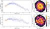Fig. 9.

Gas metallicity (top) and the SFR density (bottom), plotted as a function of distance from the centre of the galaxy on the left and as a map on the right. In the radial plots, the grey curve shows the rolling average with the shaded area representing the 1σ distribution. The colours of the points in the radial plots indicate the dominant source of ionisation in that bin according to the WHaD diagram in Fig. 8.

The negative trend across the outer disc has been seen in many star-forming galaxies (e.g. Zaritsky et al. 1994; Moustakas et al. 2010; Rupke et al. 2010; Sánchez et al. 2014; Lian et al. 2018; Franchetto et al. 2021; Valé et al. 2025) and in simulations (e.g. Tapia-Contreras et al. 2025), and is often attributed to a radial gas inflow, where the gas that is migrating inwards is being continuously enriched by ongoing star formation as it moves through the galaxy (Wang & Lilly 2022). This negative metallicity gradient across the disc is consistent with the star-forming branch in the BPT diagram in Fig. 6, in which the inner and outer parts of the disc sit on the lower and upper regions of this branch, respectively, which corresponds to higher and lower metallicities, respectively.

The inner region of the galaxy (< 3″), on the other hand, shows a positive gradient, where the gas metallicity decreases towards the centre of the galaxy. This effect has been seen before in studies of the gas metallicity gradients in CALIFA galaxies by Rosales-Ortega et al. (2011), Sánchez et al. (2012), and Sánchez et al. (2014). Sánchez et al. (2014) studied the properties of 26 galaxies with clear evidence of a drop in the gas metallicity at their cores and a further 21 galaxies with possible evidence of a drop. Through this analysis they found no clear correlation with the morphology, presence of a bar, or through recent interactions or mergers, though they could not rule out the effect of a past interaction or minor merger that is no longer visible in the morphology of the galaxy. They did, however, find that many of the galaxies displaying this feature also appear to show a central star-forming ring, detected in the Hα emission maps. They concluded that the drop in the gas metallicity in the centre of the galaxy is associated with a central star-forming ring, and that both features are produced by the radial flow of gas induced by resonances in the disc pattern speed. They further hypothesised that the apparent drop or flattening in the gas metallicity in the centres of galaxies could simply be an artifact of a ‘hump’ in the gas metallicity at a radius of ∼0.5 R_e. Sánchez-Menguiano et al. (2018) also found that the negative metallicity gradient across the discs of galaxies is often stronger in galaxies with a drop in the core region than in those without the central drop. In the case of W2246f, the continuum-subtracted Hα map, shown on the right of Fig. 1, does not show a clear ring of star formation, but there is a drop in the Hα emission in the central region of the galaxy, within a radius of ∼2″. Furthermore, the WHAN and WHaD diagrams show that this region of the galaxy is retired, and the luminosity-weighted stellar populations in Fig. 5 also show a sharp increase in the ages within a radius of 2″, further indicating a drop in the recent star formation in the central region of the galaxy. These trends (lower W_Hα and older stellar ages) are consistent with the findings of Easeman et al. (2022) for galaxies with drops in the central gas phase metallicity, and the origin of the lower gas phase metallicity is still an open question in the literature.

There are several possible explanations for the lower gas metallicity at the centre of the galaxy. For example, the galaxy could have accreted ‘pristine’ or unenriched gas into its centre, either from the disc or from an external source. Without ongoing star formation, this gas would not have been enriched in the same way as the rest of the disc, producing a dilution effect and leading to the positive metallicity gradient observed in the inner region (e.g. Ceverino et al. 2016; Sánchez-Menguiano et al. 2018). Alternatively, the more metal enriched gas could have been driven out of the galaxy in its history through past AGN activity or outflows driven by starbursts (Easeman et al. 2022). Such events may have driven enough gas out of this region to quench star formation there (inside-out quenching), and as a result the enrichment of the ISM freezes, while the rest of the disc becomes richer in metals (Ceverino et al. 2016; Belfiore et al. 2017).

6.4. Star formation rate

The final step in this part of the analysis was to measure the SFR across the galaxy. Hα emission lines are one of the best SFR indicators in star-forming galaxies observed in the optical since only young, massive stars with ages < 20 Myr produce vast numbers of photons that ionise the surrounding gas (Davies et al. 2016). Thus, the SFR calculated using Hα is largely independent of the star formation history of the galaxy (Kennicutt 1998).

In order to derive accurate measurements for the SFR, one must first consider dust extinction corrections. While the Hα line is less sensitive to dust extinction compared to other star formation indicators, such as in the UV, dust effects can still be significant, even for local galaxies (Koyama et al. 2015). We therefore used the dust-corrected Hα fluxes that we calculated in Section 6.2 to calculate the Hα luminosity, L(Hα), using

$\begin{matrix} L (H α) = 4 π d_{L}^{2} F {(H α)}_{i}, \end{matrix}$ $Mathematical equation: $$ \begin{aligned} L(H\alpha ) = 4 \pi d_L^2F(H\alpha )_i, \end{aligned} $$$ (9)

where d_L is the luminosity distance, and then the SFR was determined using the relation

$\begin{matrix} SFR (H α) = 5.5 \times 10^{- 42} L (H α) \end{matrix}$ $Mathematical equation: $$ \begin{aligned} \mathrm{SFR}({H}\alpha ) = 5.5 \times 10^{-42} L({H}\alpha ) \end{aligned} $$$ (10)

from Calzetti (2013).

Having calculated the SFR for each bin, the total SFR for the galaxy as a whole was calculated to be SFR = 0.304 ± 0.017 M_⊙, which is higher than the SFR calculated by Fan et al. (2018) of $0.09 \begin{matrix} + 0.07 \\ - 0.02 \end{matrix}$ $Mathematical equation: $ 0.09 \substack{+0.07 \\ -0.02} $$ M_⊙ using SED fitting. Generally, spectroscopic SFRs, especially those calculated using the Hα line, are most sensitive to recent or ongoing star formation since only stars with masses of > 10 M_⊙ and lifetimes of < 20 Myr contribute significantly to the integrated ionising flux (Kennicutt 1998; Calzetti et al. 2007). Thus, the SFR derived from the Hα emission traces stars with lifetimes of the order of 3 − 10 Myr (Kennicutt & Evans 2012; Flores Velázquez et al. 2021). On the other hand, SFRs calculated through SED fitting tend to be more sensitive to dust reddening and star formation over longer timescales, typically of the order of 10 − 300 Myrs, and so give a more time-averaged SFR measurement (Kennicutt & Evans 2012). Thus, the higher value measured in this work could indicate that the galaxy is undergoing a period of enhanced star formation compared to its recent history, but it is still on the low side for a typical spiral galaxy (e.g. Catalán-Torrecilla et al. 2015, 2017; Santoro et al. 2022). However, it should be noted that other factors may play a role in this discrepancy, such as aperture effects, dust treatment, and IMF assumptions.

Finally, to account for the different areas covered by each bin across the galaxy, the SFR density, Σ_SFR, was calculated. The bottom row of Fig. 9 shows the Σ_SFR as a function of radius from the centre of the galaxy, and as a map on the right of the plot. In general, the Σ_SFR is relatively flat across the disc, with a slight drop in the centre of the galaxy (r ≲ 1″) and in the outermost regions of the disc (r ≳ 6″).

For a typical star-forming galaxy, the Σ_SFR is generally ∼10⁻¹ − 10⁻³ M_⊙ yr⁻¹ kpc⁻² (Leroy et al. 2012; Cano-Díaz et al. 2016), whereas green valley regions, which are partially quenched but still forming some stars, have typical Σ_SFR ∼ 10⁻³ − 10⁻⁴ M_⊙ yr⁻¹ kpc⁻² (Belfiore et al. 2017). Moving to lower values, cLIER bulges (retired regions) in star-forming spiral galaxies have Σ_SFR ∼ 10⁻⁴ − 10⁻⁵ M_⊙ yr⁻¹ kpc⁻² (Belfiore et al. 2017), and fully retired galaxies with emission-line regions powered by HOLMES have Σ_SFR ∼ 10⁻⁵ M_⊙ yr⁻¹ kpc⁻² (González Delgado et al. 2017). Based on these values in the literature, it can be seen that W2246f appears to be a typical star-forming spiral, but with a relatively low Σ_SFR that approaches the values normally seen in green valley galaxies. Thus, these results may be pointing towards a scenario in which W2246f is in the early stages of being quenched, possibly from the inside out.

7. Summary and conclusions

In this work we present a detailed study of W2246f , a flocculent spiral galaxy that was found in the foreground of a deep MUSE datacube with a ∼20 hour exposure time. While many observations of spiral galaxies at this redshift (z ∼ 0.009) exist in surveys such as MaNGA, CALIFA, and SAMI, they lack the spatial resolution and the full coverage of the galaxy that we have in this datacube, meriting a more detailed study of its stellar and gas properties over the full extent of the galaxy.

A study of the visual morphology and the stellar and gas kinematics show no obvious signs of distortion, indicating that it is unlikely that the galaxy has undergone a recent interaction within the last 1 billion years (Hung et al. 2016; Davis & Bureau 2016). In the datacube, there does appear to be a neighbouring galaxy ∼20″ to the north-west of W2246f, but analysis of the two galaxies’ redshifts and distances revealed that they have a physical separation of ∼1 Mpc, meaning that, while they may be part of the same group or cluster of galaxies, they are too far apart to be directly interacting.

Analysis of the stellar populations showed relatively old mass-weighted ages across the whole galaxy, with older ages in the bulge-dominated region at the centre and no strong gradient across the disc, indicating that the galaxy formed the majority of its mass long ago. On the other hand, the luminosity-weighted ages show a steep negative trend in the inner 2 − 3″, with a relatively flat distribution of young stars across the rest of the disc. The stellar metallicities, both luminosity- and mass-weighted, show a negative gradient with radius across the disc, which is often seen in spiral galaxies. In the inner part of the galaxy, the mass-weighted metallicities show a slight positive gradient before decreasing again throughout the rest of the disc. This drop at the very centre coincides with the region of older luminosity-weighted stellar populations, and is consistent with the scenario in which the star formation in that region has been truncated, reducing the chemical enrichment there relative to other parts of the disc that have ongoing star formation. In the outer part of the disc the luminosity-weighted metallicities are slightly higher than the mass-weighted values, indicating stronger chemical enrichment in the younger, more recently formed stars than the older stars.

Analysis of the gas properties revealed that the gas metallicities also show a negative gradient outside of a radius of 2 − 3″, but display a positive gradient within this radius. The Σ_SFR is also relatively flat, with a slight drop in the innermost region of the galaxy. The BPT diagram was also created, which indicated that the majority of the disc is star-forming, but the central region lay in the LINER part of the diagram. A deeper analysis of the properties of the Hα emission lines using the WHAN and WHaD diagrams, which also consider the equivalent width and velocity dispersion of the Hα line, revealed that actually the centre of the galaxy is a ‘retired’ region, where the main source of ionisation is not from a LINER, but from HOLMESs.

Together, these results reflect that W2246f is a relatively normal spiral galaxy. The results indicate that the majority of its mass was created a long time ago, likely around 6 − 7 billion years ago based on the mass-weighted ages across the galaxy, and that the majority of the disc has undergone continuous star formation since then.

The central region of the galaxy, within a radius of ∼2″, is interesting though. The luminosity-weighted ages show a sharp increase in this region, indicating that the light is dominated by older stars there. These stars could come from the bulge, which is typically older than the disc (Lah et al. 2023; Jin et al. 2024; Jegatheesan et al. 2024), but could also reflect truncation or quenching of star formation in the centre of the galaxy. This scenario is also consistent with the lower Σ_SFR at the centre of the galaxy and the retired region classification from the WHAN and WHaD diagrams. The Σ_SFR is actually at the lower end of the range for typical star-forming galaxies, touching on values often seen in green valley galaxies, so it is possible that this galaxy is in the early stages of inside-out quenching.

The gas metallicity plot is also consistent with this scenario. The negative gradient in the outer disc can be explained by lower-metallicity gas being accreted into the outskirts of the galaxy and the gas generally becoming more metal-enriched by ongoing star formation as it migrates inwards through the disc. The drop in the gas metallicity in the centre could then be explained by the star formation there being slowly quenched or truncated, leading to less enrichment over time than in the regions surrounding it.

In summary, these results indicate that W2246f is a nice example of a cLIER galaxy (Belfiore et al. 2016), where the central kiloparsec or so is dominated by old, metal-poor stars with little star formation and where the central LIER emission is primarily powered by hot evolved (pAGB) stars, while the rest of the disc is displaying ongoing star formation. Often these galaxies are found to show evidence of inside-out quenching, such as is seen in W2246f The unusually deep observations with MUSE of this galaxy give us a rare opportunity to study this phenomenon with a better spatial resolution than can normally be achieved with the current IFU surveys of galaxies at a similar redshift.

Acknowledgments

We would like to thank the anonymous referee for their comments, which helped to improve the paper. This work was based on observations collected at the European Organisation for Astronomical Research in the Southern Hemisphere under ESO programmes 106.21F0.001 (PI Diaz-Santos) and 109.2393.001 (PI Assef). This research has made use of the NASA/IPAC Infrared Science Archive, which is funded by the National Aeronautics and Space Administration and operated by the California Institute of Technology. E.J.J, S.L., R.J.A, M.A. and D.S. acknowledge the support from the ANID CATA-BASAL project FB210003. E.J.J was supported by FONDECYT Regular grant number 1262304. A.Z.L.A. gratefully acknowledges the support provided by the Postdoctoral Program (POSDOC) of UNAM (Universidad Nacional Autónoma de México). M.A. is supported by FONDECYT grant number 1252054, and gratefully acknowledges support from ANID MILENIO NCN2024_112 and ANID + Vinculación Internacional + FOVI250261. R.J.A was supported by FONDECYT grant number 1231718. M.L. was supported by the grants from the Rubin-Chile Fund (DIA3324). D.S. was supported by the ALMA-ANID grant number 31220030.

References

Agostino, C. J., & Salim, S. 2019, ApJ, 876, 12 [NASA ADS] [CrossRef] [Google Scholar]
Aragon Calvo, M. A., Neyrinck, M. C., & Silk, J. 2019, Open J. Astrophys., 2, 7 [CrossRef] [Google Scholar]
Aragon-Calvo, M. A., & Szalay, A. S. 2013, MNRAS, 428, 3409 [NASA ADS] [CrossRef] [Google Scholar]
Bacon, R., Accardo, M., Adjali, L., et al. 2010, SPIE Conf. Ser., 7735, 773508 [Google Scholar]
Baldwin, J. A., Phillips, M. M., & Terlevich, R. 1981, PASP, 93, 5 [Google Scholar]
Bao, M., Chen, Y., Zhu, P., et al. 2022, ApJ, 926, L13 [CrossRef] [Google Scholar]
Belfiore, F., Maiolino, R., Bundy, K., et al. 2015, MNRAS, 449, 867 [NASA ADS] [CrossRef] [Google Scholar]
Belfiore, F., Maiolino, R., Maraston, C., et al. 2016, MNRAS, 461, 3111 [Google Scholar]
Belfiore, F., Maiolino, R., Tremonti, C., et al. 2017, MNRAS, 469, 151 [Google Scholar]
Binette, L., Magris, C. G., Stasińska, G., & Bruzual, A. G. 1994, A&A, 292, 13 [NASA ADS] [Google Scholar]
Borlaff, A., Eliche-Moral, M. C., Rodríguez-Pérez, C., et al. 2014, A&A, 570, A103 [NASA ADS] [CrossRef] [EDP Sciences] [Google Scholar]
Brandt, T. D., Tojeiro, R., Aubourg, É., et al. 2010, AJ, 140, 804 [Google Scholar]
Breda, I., Papaderos, P., Gomes, J. M., et al. 2020, A&A, 635, A177 [NASA ADS] [CrossRef] [EDP Sciences] [Google Scholar]
Bryant, J. J., Owers, M. S., Robotham, A. S. G., et al. 2015, MNRAS, 447, 2857 [Google Scholar]
Bundy, K., Bershady, M. A., Law, D. R., et al. 2015, ApJ, 798, 7 [Google Scholar]
Byrne-Mamahit, S., Patton, D. R., Ellison, S. L., et al. 2024, MNRAS, 528, 5864 [Google Scholar]
Calzetti, D. 2013, in Secular Evolution of Galaxies, eds. J. Falcón-Barroso, & J. H. Knapen, 419 [Google Scholar]
Calzetti, D., Armus, L., Bohlin, R. C., et al. 2000, ApJ, 533, 682 [NASA ADS] [CrossRef] [Google Scholar]
Calzetti, D., Kennicutt, R. C., Engelbracht, C. W., et al. 2007, ApJ, 666, 870 [Google Scholar]
Cano-Díaz, M., Sánchez, S. F., Zibetti, S., et al. 2016, ApJ, 821, L26 [Google Scholar]
Cappellari, M. 2017, MNRAS, 466, 798 [Google Scholar]
Cappellari, M. 2023, MNRAS, 526, 3273 [NASA ADS] [CrossRef] [Google Scholar]
Cappellari, M. 2025, MNRAS, 544, 1432 [Google Scholar]
Cardelli, J. A., Clayton, G. C., & Mathis, J. S. 1989, ApJ, 345, 245 [Google Scholar]
Casteels, K. R. V., Bamford, S. P., Skibba, R. A., et al. 2013, MNRAS, 429, 1051 [NASA ADS] [CrossRef] [Google Scholar]
Catalán-Torrecilla, C., Gil de Paz, A., Castillo-Morales, A., et al. 2015, A&A, 584, A87 [NASA ADS] [CrossRef] [EDP Sciences] [Google Scholar]
Catalán-Torrecilla, C., Gil de Paz, A., Castillo-Morales, A., et al. 2017, ApJ, 848, 87 [Google Scholar]
Ceverino, D., Sánchez Almeida, J., Muñoz Tuñón, C., et al. 2016, MNRAS, 457, 2605 [NASA ADS] [CrossRef] [Google Scholar]
Chernin, A. D., Dolgachev, V. P., & Domozhilova, L. M. 2000, MNRAS, 319, 851 [Google Scholar]
Cid Fernandes, R., Stasińska, G., Mateus, A., & Vale Asari, N. 2011, MNRAS, 413, 1687 [Google Scholar]
Cid Fernandes, R., Carvalho, M. S., Sánchez, S. F., de Amorim, A., & Ruschel-Dutra, D. 2021, MNRAS, 502, 1386 [NASA ADS] [CrossRef] [Google Scholar]
Croom, S. M., Lawrence, J. S., Bland-Hawthorn, J., et al. 2012, MNRAS, 421, 872 [NASA ADS] [Google Scholar]
Curti, M., Hayden-Pawson, C., Maiolino, R., et al. 2022, MNRAS, 512, 4136 [NASA ADS] [CrossRef] [Google Scholar]
Davies, L. J. M., Driver, S. P., Robotham, A. S. G., et al. 2016, MNRAS, 461, 458 [NASA ADS] [CrossRef] [Google Scholar]
Davis, T. A., & Bureau, M. 2016, MNRAS, 457, 272 [Google Scholar]
Di Matteo, P., Haywood, M., Combes, F., Semelin, B., & Snaith, O. N. 2013, A&A, 553, A102 [NASA ADS] [CrossRef] [EDP Sciences] [Google Scholar]
Díaz-Santos, T., Assef, R. J., Blain, A. W., et al. 2016, ApJ, 816, L6 [Google Scholar]
Díaz-Santos, T., Assef, R. J., Blain, A. W., et al. 2018, Science, 362, 1034 [Google Scholar]
Domínguez, A., Siana, B., Henry, A. L., et al. 2013, ApJ, 763, 145 [CrossRef] [Google Scholar]
Dopita, M. A., & Sutherland, R. S. 1996, ApJS, 102, 161 [Google Scholar]
Drory, N., Blanc, G. A., Kreckel, K., et al. 2024, AJ, 168, 198 [NASA ADS] [CrossRef] [Google Scholar]
Easeman, B., Schady, P., Wuyts, S., & Yates, R. M. 2022, MNRAS, 511, 371 [NASA ADS] [CrossRef] [Google Scholar]
Ebrová, I., Bílek, M., & Eliášek, J. 2025, A&A, 704, A232 [NASA ADS] [CrossRef] [EDP Sciences] [Google Scholar]
Egorova, E., Kreckel, K., Egorov, O., et al. 2026, A&A, 705, A45 [NASA ADS] [CrossRef] [EDP Sciences] [Google Scholar]
Eliche-Moral, M. C., Rodríguez-Pérez, C., Borlaff, A., Querejeta, M., & Tapia, T. 2018, A&A, 617, A113 [NASA ADS] [CrossRef] [EDP Sciences] [Google Scholar]
Ellison, S. L., Patton, D. R., Simard, L., & McConnachie, A. W. 2008, AJ, 135, 1877 [NASA ADS] [CrossRef] [Google Scholar]
Emsellem, E., Schinnerer, E., Santoro, F., et al. 2022, A&A, 659, A191 [NASA ADS] [CrossRef] [EDP Sciences] [Google Scholar]
Erroz-Ferrer, S., Carollo, C. M., den Brok, M., et al. 2019, MNRAS, 484, 5009 [Google Scholar]
ESO CPL Development Team. 2015, Astrophysics Source Code Library [record ascl:1504.003] [Google Scholar]
Fan, L., Gao, Y., Knudsen, K. K., & Shu, X. 2018, ApJ, 854, 157 [NASA ADS] [CrossRef] [Google Scholar]
Fensch, J., Duc, P.-A., Weilbacher, P. M., Boquien, M., & Zackrisson, E. 2016, A&A, 585, A79 [NASA ADS] [CrossRef] [EDP Sciences] [Google Scholar]
Fitzpatrick, E. L. 1999, PASP, 111, 63 [Google Scholar]
Flores Velázquez, J. A., Gurvich, A. B., Faucher-Giguère, C.-A., et al. 2021, MNRAS, 501, 4812 [CrossRef] [Google Scholar]
Flores-Fajardo, N., Morisset, C., Stasińska, G., & Binette, L. 2011, MNRAS, 415, 2182 [Google Scholar]
Franchetto, A., Mingozzi, M., Poggianti, B. M., et al. 2021, ApJ, 923, 28 [NASA ADS] [CrossRef] [Google Scholar]
Gadotti, D. A., Sánchez-Blázquez, P., Falcón-Barroso, J., et al. 2019, MNRAS, 482, 506 [Google Scholar]
Gadotti, D. A., Bittner, A., Falcón-Barroso, J., et al. 2020, A&A, 643, A14 [NASA ADS] [CrossRef] [EDP Sciences] [Google Scholar]
Gibson, B. K. 1997, MNRAS, 290, 471 [NASA ADS] [Google Scholar]
Goddard, D., Thomas, D., Maraston, C., et al. 2017, MNRAS, 466, 4731 [NASA ADS] [Google Scholar]
González Delgado, R. M., Pérez, E., Cid Fernandes, R., et al. 2017, A&A, 607, A128 [NASA ADS] [CrossRef] [EDP Sciences] [Google Scholar]
Green, A. W., Glazebrook, K., McGregor, P. J., et al. 2010, Nature, 467, 684 [NASA ADS] [CrossRef] [Google Scholar]
Green, A. W., Glazebrook, K., McGregor, P. J., et al. 2014, MNRAS, 437, 1070 [Google Scholar]
Groves, B., Brinchmann, J., & Walcher, C. J. 2012, MNRAS, 419, 1402 [NASA ADS] [CrossRef] [Google Scholar]
Harikane, Y., Zhang, Y., Nakajima, K., et al. 2023, ApJ, 959, 39 [NASA ADS] [CrossRef] [Google Scholar]
Häußler, B., McIntosh, D. H., Barden, M., et al. 2007, ApJS, 172, 615 [NASA ADS] [CrossRef] [Google Scholar]
Häußler, B., Bamford, S. P., Vika, M., et al. 2013, MNRAS, 430, 330 [Google Scholar]
Hill, G. J., Lee, H., MacQueen, P. J., et al. 2021, AJ, 162, 298 [NASA ADS] [CrossRef] [Google Scholar]
Hummer, D. G., & Storey, P. J. 1987, MNRAS, 224, 801 [NASA ADS] [CrossRef] [Google Scholar]
Hung, C.-L., Hayward, C. C., Smith, H. A., et al. 2016, ApJ, 816, 99 [NASA ADS] [CrossRef] [Google Scholar]
Jegatheesan, K., Johnston, E. J., Häußler, B., & Nedkova, K. V. 2024, A&A, 684, A32 [NASA ADS] [CrossRef] [EDP Sciences] [Google Scholar]
Jin, Y., Zhu, L., Zibetti, S., et al. 2024, A&A, 681, A95 [NASA ADS] [CrossRef] [EDP Sciences] [Google Scholar]
Johnston, E. J., Hau, G. K. T., Coccato, L., & Herrera, C. 2018, MNRAS, 480, 3215 [Google Scholar]
Kauffmann, G., Heckman, T. M., Tremonti, C., et al. 2003, MNRAS, 346, 1055 [Google Scholar]
Kennicutt, R. C., Jr. 1998, ApJ, 498, 541 [Google Scholar]
Kennicutt, R. C., & Evans, N. J. 2012, ARA&A, 50, 531 [NASA ADS] [CrossRef] [Google Scholar]
Kewley, L. J., Dopita, M. A., Sutherland, R. S., Heisler, C. A., & Trevena, J. 2001, ApJ, 556, 121 [Google Scholar]
Kewley, L. J., Groves, B., Kauffmann, G., & Heckman, T. 2006, MNRAS, 372, 961 [Google Scholar]
Kocevski, D. D., Onoue, M., Inayoshi, K., et al. 2023, ApJ, 954, L4 [NASA ADS] [CrossRef] [Google Scholar]
Koyama, Y., Kodama, T., Hayashi, M., et al. 2015, MNRAS, 453, 879 [Google Scholar]
Krajnović, D., Weilbacher, P. M., Urrutia, T., et al. 2015, MNRAS, 452, 2 [Google Scholar]
Lacerda, E. A. D., Cid Fernandes, R., Couto, G. S., et al. 2018, MNRAS, 474, 3727 [Google Scholar]
Lah, P., Scott, N., Barone, T. M., et al. 2023, PASA, 40, e002 [Google Scholar]
Lara-López, M. A., Galán-de Anta, P. M., Sarzi, M., et al. 2022, A&A, 660, A105 [NASA ADS] [CrossRef] [EDP Sciences] [Google Scholar]
Lelli, F., Fraternali, F., & Sancisi, R. 2010, A&A, 516, A11 [NASA ADS] [CrossRef] [EDP Sciences] [Google Scholar]
Leroy, A. K., Bigiel, F., de Blok, W. J. G., et al. 2012, AJ, 144, 3 [Google Scholar]
Li, C., Kauffmann, G., Heckman, T. M., Jing, Y. P., & White, S. D. M. 2008, MNRAS, 385, 1903 [NASA ADS] [CrossRef] [Google Scholar]
Lian, J., Thomas, D., Maraston, C., et al. 2018, MNRAS, 476, 3883 [NASA ADS] [CrossRef] [Google Scholar]
López-Cobá, C., Sánchez, S. F., Anderson, J. P., et al. 2020, AJ, 159, 167 [Google Scholar]
Ma, J., Maksym, W. P., Fabbiano, G., et al. 2021, ApJ, 908, 155 [Google Scholar]
Maiolino, R., Scholtz, J., Curtis-Lake, E., et al. 2024, A&A, 691, A145 [NASA ADS] [CrossRef] [EDP Sciences] [Google Scholar]
Mannucci, F., Della Valle, M., Panagia, N., et al. 2005, A&A, 433, 807 [NASA ADS] [CrossRef] [EDP Sciences] [Google Scholar]
Maoz, D., & Mannucci, F. 2012, PASA, 29, 447 [NASA ADS] [CrossRef] [Google Scholar]
Maoz, D., Mannucci, F., Li, W., et al. 2011, MNRAS, 412, 1508 [Google Scholar]
Marconcini, C., Feltre, A., Lamperti, I., et al. 2025, A&A, 701, A113 [NASA ADS] [CrossRef] [EDP Sciences] [Google Scholar]
Marino, R. A., Rosales-Ortega, F. F., Sánchez, S. F., et al. 2013, A&A, 559, A114 [NASA ADS] [CrossRef] [EDP Sciences] [Google Scholar]
Martínez-Delgado, D., Stein, M., Sakowska, J. D., et al. 2025, A&A, 701, A182 [NASA ADS] [CrossRef] [EDP Sciences] [Google Scholar]
Matteucci, F., & Francois, P. 1989, MNRAS, 239, 885 [Google Scholar]
Matteucci, F., Spitoni, E., Recchi, S., & Valiante, R. 2009, A&A, 501, 531 [NASA ADS] [CrossRef] [EDP Sciences] [Google Scholar]
Medling, A. M., U, V., Guedes, J., et al. 2014, ApJ, 784, 70 [Google Scholar]
Michel-Dansac, L., Lambas, D. G., Alonso, M. S., & Tissera, P. 2008, MNRAS, 386, L82 [NASA ADS] [CrossRef] [Google Scholar]
Moustakas, J., Kennicutt, R. C., Jr., Tremonti, C. A., et al. 2010, ApJS, 190, 233 [Google Scholar]
Naab, T., Oser, L., Emsellem, E., et al. 2014, MNRAS, 444, 3357 [Google Scholar]
Nakajima, K., & Maiolino, R. 2022, MNRAS, 513, 5134 [NASA ADS] [CrossRef] [Google Scholar]
Nedelchev, B., Coccato, L., Corsini, E. M., et al. 2019, A&A, 623, A87 [NASA ADS] [CrossRef] [EDP Sciences] [Google Scholar]
Nedkova, K. V., Häußler, B., Marchesini, D., et al. 2021, MNRAS, 506, 928 [NASA ADS] [CrossRef] [Google Scholar]
Nikolic, B., Cullen, H., & Alexander, P. 2004, MNRAS, 355, 874 [NASA ADS] [CrossRef] [Google Scholar]
Osterbrock, D. E. 1989, Astrophysics of Gaseous Nebulae and Active Galactic Nuclei (University Science Books) [Google Scholar]
Parikh, T., Thomas, D., Maraston, C., et al. 2021, MNRAS, 502, 5508 [NASA ADS] [CrossRef] [Google Scholar]
Patton, D. R., Ellison, S. L., Simard, L., McConnachie, A. W., & Mendel, J. T. 2011, MNRAS, 412, 591 [NASA ADS] [CrossRef] [Google Scholar]
Patton, D. R., Faria, L., Hani, M. H., et al. 2024, MNRAS, 529, 1493 [Google Scholar]
Peng, C. Y., Ho, L. C., Impey, C. D., & Rix, H.-W. 2002, AJ, 124, 266 [Google Scholar]
Peng, C. Y., Ho, L. C., Impey, C. D., & Rix, H.-W. 2010, AJ, 139, 2097 [Google Scholar]
Pérez-Montero, E., & Contini, T. 2009, MNRAS, 398, 949 [CrossRef] [Google Scholar]
Pessa, I., Schinnerer, E., Sanchez-Blazquez, P., et al. 2023, A&A, 673, A147 [NASA ADS] [CrossRef] [EDP Sciences] [Google Scholar]
Peterken, T., Merrifield, M., Aragón-Salamanca, A., et al. 2020, MNRAS, 495, 3387 [Google Scholar]
Pettini, M., & Pagel, B. E. J. 2004, MNRAS, 348, L59 [NASA ADS] [CrossRef] [Google Scholar]
Pilyugin, L. S., Zinchenko, I. A., Lara-López, M. A., Nefedyev, Y. A., & Vílchez, J. M. 2021, A&A, 646, A54 [NASA ADS] [CrossRef] [EDP Sciences] [Google Scholar]
Robaina, A. R., Bell, E. F., Skelton, R. E., et al. 2009, ApJ, 704, 324 [NASA ADS] [CrossRef] [Google Scholar]
Rosales-Ortega, F. F., Díaz, A. I., Kennicutt, R. C., & Sánchez, S. F. 2011, MNRAS, 415, 2439 [NASA ADS] [CrossRef] [Google Scholar]
Ruiz-Lara, T., Pérez, I., Florido, E., et al. 2017, A&A, 604, A4 [NASA ADS] [CrossRef] [EDP Sciences] [Google Scholar]
Rupke, D. S. N., Kewley, L. J., & Chien, L.-H. 2010, ApJ, 723, 1255 [NASA ADS] [CrossRef] [Google Scholar]
Sánchez, S. F. 2020, ARA&A, 58, 99 [Google Scholar]
Sánchez, S. F., Rosales-Ortega, F. F., Marino, R. A., et al. 2012, A&A, 546, A2 [NASA ADS] [CrossRef] [EDP Sciences] [Google Scholar]
Sánchez, S. F., Rosales-Ortega, F. F., Iglesias-Páramo, J., et al. 2014, A&A, 563, A49 [CrossRef] [EDP Sciences] [Google Scholar]
Sánchez, S. F., García-Benito, R., Zibetti, S., et al. 2016, A&A, 594, A36 [Google Scholar]
Sánchez, S. F., Lugo-Aranda, A. Z., Sánchez Almeida, J., et al. 2024, A&A, 682, A71 [NASA ADS] [CrossRef] [EDP Sciences] [Google Scholar]
Sánchez-Blázquez, P., Rosales-Ortega, F. F., Méndez-Abreu, J., et al. 2014, A&A, 570, A6 [NASA ADS] [CrossRef] [EDP Sciences] [Google Scholar]
Sánchez-Menguiano, L., Sánchez, S. F., Pérez, I., et al. 2018, A&A, 609, A119 [NASA ADS] [CrossRef] [EDP Sciences] [Google Scholar]
Santoro, F., Kreckel, K., Belfiore, F., et al. 2022, A&A, 658, A188 [NASA ADS] [CrossRef] [EDP Sciences] [Google Scholar]
Scannapieco, E., & Bildsten, L. 2005, ApJ, 629, L85 [Google Scholar]
Schlafly, E. F., & Finkbeiner, D. P. 2011, ApJ, 737, 103 [Google Scholar]
Shah, E. A., Kartaltepe, J. S., Magagnoli, C. T., et al. 2022, ApJ, 940, 4 [NASA ADS] [CrossRef] [Google Scholar]
Singh, R., van de Ven, G., Jahnke, K., et al. 2013, A&A, 558, A43 [NASA ADS] [CrossRef] [EDP Sciences] [Google Scholar]
Soto, K. T., Lilly, S. J., Bacon, R., Richard, J., & Conseil, S. 2016, MNRAS, 458, 3210 [Google Scholar]
Stasińska, G., Vale Asari, N., Cid Fernandes, R., et al. 2008, MNRAS, 391, L29 [NASA ADS] [Google Scholar]
Sullivan, M., Le Borgne, D., Pritchet, C. J., et al. 2006, ApJ, 648, 868 [NASA ADS] [CrossRef] [Google Scholar]
Tapia-Contreras, B., Tissera, P. B., Sillero, E., et al. 2025, A&A, 700, A69 [NASA ADS] [CrossRef] [EDP Sciences] [Google Scholar]
Tissera, P. B., Machado, R. E. G., Sanchez-Blazquez, P., et al. 2016, A&A, 592, A93 [NASA ADS] [CrossRef] [EDP Sciences] [Google Scholar]
Tsai, C.-W., Eisenhardt, P. R. M., Wu, J., et al. 2015, ApJ, 805, 90 [Google Scholar]
Tsai, C.-W., Eisenhardt, P. R. M., Jun, H. D., et al. 2018, ApJ, 868, 15 [NASA ADS] [CrossRef] [Google Scholar]
Übler, H., Maiolino, R., Curtis-Lake, E., et al. 2023, A&A, 677, A145 [NASA ADS] [CrossRef] [EDP Sciences] [Google Scholar]
Valé, G., Lara-López, M. A., Valerdi, M., et al. 2025, A&A, 701, A226 [NASA ADS] [CrossRef] [EDP Sciences] [Google Scholar]
van de Sande, J., Bland-Hawthorn, J., Fogarty, L. M. R., et al. 2017, ApJ, 835, 104 [Google Scholar]
Vazdekis, A., Koleva, M., Ricciardelli, E., Röck, B., & Falcón-Barroso, J. 2016, MNRAS, 463, 3409 [Google Scholar]
Veilleux, S., & Osterbrock, D. E. 1987, ApJS, 63, 295 [Google Scholar]
Venturi, G., Marconi, A., Mingozzi, M., et al. 2017, Front. Astron. Space Sci., 4, 46 [Google Scholar]
Wang, E., & Lilly, S. J. 2022, ApJ, 929, 95 [Google Scholar]
Weilbacher, P. M., Streicher, O., Urrutia, T., et al. 2012, Proc. SPIE, 8451, 84510B [NASA ADS] [CrossRef] [Google Scholar]
Wu, J., Tsai, C.-W., Sayers, J., et al. 2012, ApJ, 756, 96 [Google Scholar]
Yu, X., Shi, Y., Chen, Y., et al. 2019, MNRAS, 486, 4463 [Google Scholar]
Zaritsky, D., Kennicutt, R. C., Jr., & Huchra, J. P. 1994, ApJ, 420, 87 [NASA ADS] [CrossRef] [Google Scholar]

http://skyserver.sdss.org/

https://irsa.ipac.caltech.edu/applications/DUST/

All Figures

Fig. 1.

In the text

	Fig. 2. Maps of the stellar (top) and gas (bottom) kinematics, showing from left to right the line of sight velocities, velocity dispersions and h₃ and h₄ coefficients for W2246f. The contours represent the flux in the white light image for reference, and the axes labels represent the distance in arcseconds from the centre of the galaxy.
In the text

	Fig. 3. Maps showing the stellar line-of-sight velocities (left) and velocity dispersions (right) for the neighbouring galaxy to W2246f. The contours represent the flux in the white light image for reference.
In the text

	Fig. 7. Reddening (left) and extinction (right) maps of W2246f.
In the text

Current usage metrics show cumulative count of Article Views (full-text article views including HTML views, PDF and ePub downloads, according to the available data) and Abstracts Views on Vision4Press platform.

Data correspond to usage on the plateform after 2015. The current usage metrics is available 48-96 hours after online publication and is updated daily on week days.

Initial download of the metrics may take a while.

[R1] Agostino, C. J., & Salim, S. 2019, ApJ, 876, 12 [NASA ADS] [CrossRef] [Google Scholar]

[R2] Aragon Calvo, M. A., Neyrinck, M. C., & Silk, J. 2019, Open J. Astrophys., 2, 7 [CrossRef] [Google Scholar]

[R3] Aragon-Calvo, M. A., & Szalay, A. S. 2013, MNRAS, 428, 3409 [NASA ADS] [CrossRef] [Google Scholar]

[R4] Bacon, R., Accardo, M., Adjali, L., et al. 2010, SPIE Conf. Ser., 7735, 773508 [Google Scholar]

[R5] Baldwin, J. A., Phillips, M. M., & Terlevich, R. 1981, PASP, 93, 5 [Google Scholar]

[R6] Bao, M., Chen, Y., Zhu, P., et al. 2022, ApJ, 926, L13 [CrossRef] [Google Scholar]

[R7] Belfiore, F., Maiolino, R., Bundy, K., et al. 2015, MNRAS, 449, 867 [NASA ADS] [CrossRef] [Google Scholar]

[R8] Belfiore, F., Maiolino, R., Maraston, C., et al. 2016, MNRAS, 461, 3111 [Google Scholar]

[R9] Belfiore, F., Maiolino, R., Tremonti, C., et al. 2017, MNRAS, 469, 151 [Google Scholar]

[R10] Binette, L., Magris, C. G., Stasińska, G., & Bruzual, A. G. 1994, A&A, 292, 13 [NASA ADS] [Google Scholar]

[R11] Borlaff, A., Eliche-Moral, M. C., Rodríguez-Pérez, C., et al. 2014, A&A, 570, A103 [NASA ADS] [CrossRef] [EDP Sciences] [Google Scholar]

[R12] Brandt, T. D., Tojeiro, R., Aubourg, É., et al. 2010, AJ, 140, 804 [Google Scholar]

[R13] Breda, I., Papaderos, P., Gomes, J. M., et al. 2020, A&A, 635, A177 [NASA ADS] [CrossRef] [EDP Sciences] [Google Scholar]

[R14] Bryant, J. J., Owers, M. S., Robotham, A. S. G., et al. 2015, MNRAS, 447, 2857 [Google Scholar]

[R15] Bundy, K., Bershady, M. A., Law, D. R., et al. 2015, ApJ, 798, 7 [Google Scholar]

[R16] Byrne-Mamahit, S., Patton, D. R., Ellison, S. L., et al. 2024, MNRAS, 528, 5864 [Google Scholar]

[R17] Calzetti, D. 2013, in Secular Evolution of Galaxies, eds. J. Falcón-Barroso, & J. H. Knapen, 419 [Google Scholar]

[R18] Calzetti, D., Armus, L., Bohlin, R. C., et al. 2000, ApJ, 533, 682 [NASA ADS] [CrossRef] [Google Scholar]

[R19] Calzetti, D., Kennicutt, R. C., Engelbracht, C. W., et al. 2007, ApJ, 666, 870 [Google Scholar]

[R20] Cano-Díaz, M., Sánchez, S. F., Zibetti, S., et al. 2016, ApJ, 821, L26 [Google Scholar]

[R21] Cappellari, M. 2017, MNRAS, 466, 798 [Google Scholar]

[R22] Cappellari, M. 2023, MNRAS, 526, 3273 [NASA ADS] [CrossRef] [Google Scholar]

[R23] Cappellari, M. 2025, MNRAS, 544, 1432 [Google Scholar]

[R24] Cardelli, J. A., Clayton, G. C., & Mathis, J. S. 1989, ApJ, 345, 245 [Google Scholar]

[R25] Casteels, K. R. V., Bamford, S. P., Skibba, R. A., et al. 2013, MNRAS, 429, 1051 [NASA ADS] [CrossRef] [Google Scholar]

[R26] Catalán-Torrecilla, C., Gil de Paz, A., Castillo-Morales, A., et al. 2015, A&A, 584, A87 [NASA ADS] [CrossRef] [EDP Sciences] [Google Scholar]

[R27] Catalán-Torrecilla, C., Gil de Paz, A., Castillo-Morales, A., et al. 2017, ApJ, 848, 87 [Google Scholar]

[R28] Ceverino, D., Sánchez Almeida, J., Muñoz Tuñón, C., et al. 2016, MNRAS, 457, 2605 [NASA ADS] [CrossRef] [Google Scholar]

[R29] Chernin, A. D., Dolgachev, V. P., & Domozhilova, L. M. 2000, MNRAS, 319, 851 [Google Scholar]

[R30] Cid Fernandes, R., Stasińska, G., Mateus, A., & Vale Asari, N. 2011, MNRAS, 413, 1687 [Google Scholar]

[R31] Cid Fernandes, R., Carvalho, M. S., Sánchez, S. F., de Amorim, A., & Ruschel-Dutra, D. 2021, MNRAS, 502, 1386 [NASA ADS] [CrossRef] [Google Scholar]

[R32] Croom, S. M., Lawrence, J. S., Bland-Hawthorn, J., et al. 2012, MNRAS, 421, 872 [NASA ADS] [Google Scholar]

[R33] Curti, M., Hayden-Pawson, C., Maiolino, R., et al. 2022, MNRAS, 512, 4136 [NASA ADS] [CrossRef] [Google Scholar]

[R34] Davies, L. J. M., Driver, S. P., Robotham, A. S. G., et al. 2016, MNRAS, 461, 458 [NASA ADS] [CrossRef] [Google Scholar]

[R35] Davis, T. A., & Bureau, M. 2016, MNRAS, 457, 272 [Google Scholar]

[R36] Di Matteo, P., Haywood, M., Combes, F., Semelin, B., & Snaith, O. N. 2013, A&A, 553, A102 [NASA ADS] [CrossRef] [EDP Sciences] [Google Scholar]

[R37] Díaz-Santos, T., Assef, R. J., Blain, A. W., et al. 2016, ApJ, 816, L6 [Google Scholar]

[R38] Díaz-Santos, T., Assef, R. J., Blain, A. W., et al. 2018, Science, 362, 1034 [Google Scholar]

[R39] Domínguez, A., Siana, B., Henry, A. L., et al. 2013, ApJ, 763, 145 [CrossRef] [Google Scholar]

[R40] Dopita, M. A., & Sutherland, R. S. 1996, ApJS, 102, 161 [Google Scholar]

[R41] Drory, N., Blanc, G. A., Kreckel, K., et al. 2024, AJ, 168, 198 [NASA ADS] [CrossRef] [Google Scholar]

[R42] Easeman, B., Schady, P., Wuyts, S., & Yates, R. M. 2022, MNRAS, 511, 371 [NASA ADS] [CrossRef] [Google Scholar]

[R43] Ebrová, I., Bílek, M., & Eliášek, J. 2025, A&A, 704, A232 [NASA ADS] [CrossRef] [EDP Sciences] [Google Scholar]

[R44] Egorova, E., Kreckel, K., Egorov, O., et al. 2026, A&A, 705, A45 [NASA ADS] [CrossRef] [EDP Sciences] [Google Scholar]

[R45] Eliche-Moral, M. C., Rodríguez-Pérez, C., Borlaff, A., Querejeta, M., & Tapia, T. 2018, A&A, 617, A113 [NASA ADS] [CrossRef] [EDP Sciences] [Google Scholar]

[R46] Ellison, S. L., Patton, D. R., Simard, L., & McConnachie, A. W. 2008, AJ, 135, 1877 [NASA ADS] [CrossRef] [Google Scholar]

[R47] Emsellem, E., Schinnerer, E., Santoro, F., et al. 2022, A&A, 659, A191 [NASA ADS] [CrossRef] [EDP Sciences] [Google Scholar]

[R48] Erroz-Ferrer, S., Carollo, C. M., den Brok, M., et al. 2019, MNRAS, 484, 5009 [Google Scholar]

[R49] ESO CPL Development Team. 2015, Astrophysics Source Code Library [record ascl:1504.003] [Google Scholar]

[R50] Fan, L., Gao, Y., Knudsen, K. K., & Shu, X. 2018, ApJ, 854, 157 [NASA ADS] [CrossRef] [Google Scholar]

[R51] Fensch, J., Duc, P.-A., Weilbacher, P. M., Boquien, M., & Zackrisson, E. 2016, A&A, 585, A79 [NASA ADS] [CrossRef] [EDP Sciences] [Google Scholar]

[R52] Fitzpatrick, E. L. 1999, PASP, 111, 63 [Google Scholar]

[R53] Flores Velázquez, J. A., Gurvich, A. B., Faucher-Giguère, C.-A., et al. 2021, MNRAS, 501, 4812 [CrossRef] [Google Scholar]

[R54] Flores-Fajardo, N., Morisset, C., Stasińska, G., & Binette, L. 2011, MNRAS, 415, 2182 [Google Scholar]

[R55] Franchetto, A., Mingozzi, M., Poggianti, B. M., et al. 2021, ApJ, 923, 28 [NASA ADS] [CrossRef] [Google Scholar]

[R56] Gadotti, D. A., Sánchez-Blázquez, P., Falcón-Barroso, J., et al. 2019, MNRAS, 482, 506 [Google Scholar]

[R57] Gadotti, D. A., Bittner, A., Falcón-Barroso, J., et al. 2020, A&A, 643, A14 [NASA ADS] [CrossRef] [EDP Sciences] [Google Scholar]

[R58] Gibson, B. K. 1997, MNRAS, 290, 471 [NASA ADS] [Google Scholar]

[R59] Goddard, D., Thomas, D., Maraston, C., et al. 2017, MNRAS, 466, 4731 [NASA ADS] [Google Scholar]

[R60] González Delgado, R. M., Pérez, E., Cid Fernandes, R., et al. 2017, A&A, 607, A128 [NASA ADS] [CrossRef] [EDP Sciences] [Google Scholar]

[R61] Green, A. W., Glazebrook, K., McGregor, P. J., et al. 2010, Nature, 467, 684 [NASA ADS] [CrossRef] [Google Scholar]

[R62] Green, A. W., Glazebrook, K., McGregor, P. J., et al. 2014, MNRAS, 437, 1070 [Google Scholar]

[R63] Groves, B., Brinchmann, J., & Walcher, C. J. 2012, MNRAS, 419, 1402 [NASA ADS] [CrossRef] [Google Scholar]

[R64] Harikane, Y., Zhang, Y., Nakajima, K., et al. 2023, ApJ, 959, 39 [NASA ADS] [CrossRef] [Google Scholar]

[R65] Häußler, B., McIntosh, D. H., Barden, M., et al. 2007, ApJS, 172, 615 [NASA ADS] [CrossRef] [Google Scholar]

[R66] Häußler, B., Bamford, S. P., Vika, M., et al. 2013, MNRAS, 430, 330 [Google Scholar]

[R67] Hill, G. J., Lee, H., MacQueen, P. J., et al. 2021, AJ, 162, 298 [NASA ADS] [CrossRef] [Google Scholar]

[R68] Hummer, D. G., & Storey, P. J. 1987, MNRAS, 224, 801 [NASA ADS] [CrossRef] [Google Scholar]

[R69] Hung, C.-L., Hayward, C. C., Smith, H. A., et al. 2016, ApJ, 816, 99 [NASA ADS] [CrossRef] [Google Scholar]

[R70] Jegatheesan, K., Johnston, E. J., Häußler, B., & Nedkova, K. V. 2024, A&A, 684, A32 [NASA ADS] [CrossRef] [EDP Sciences] [Google Scholar]

[R71] Jin, Y., Zhu, L., Zibetti, S., et al. 2024, A&A, 681, A95 [NASA ADS] [CrossRef] [EDP Sciences] [Google Scholar]

[R72] Johnston, E. J., Hau, G. K. T., Coccato, L., & Herrera, C. 2018, MNRAS, 480, 3215 [Google Scholar]

[R73] Kauffmann, G., Heckman, T. M., Tremonti, C., et al. 2003, MNRAS, 346, 1055 [Google Scholar]

[R74] Kennicutt, R. C., Jr. 1998, ApJ, 498, 541 [Google Scholar]

[R75] Kennicutt, R. C., & Evans, N. J. 2012, ARA&A, 50, 531 [NASA ADS] [CrossRef] [Google Scholar]

[R76] Kewley, L. J., Dopita, M. A., Sutherland, R. S., Heisler, C. A., & Trevena, J. 2001, ApJ, 556, 121 [Google Scholar]

[R77] Kewley, L. J., Groves, B., Kauffmann, G., & Heckman, T. 2006, MNRAS, 372, 961 [Google Scholar]

[R78] Kocevski, D. D., Onoue, M., Inayoshi, K., et al. 2023, ApJ, 954, L4 [NASA ADS] [CrossRef] [Google Scholar]

[R79] Koyama, Y., Kodama, T., Hayashi, M., et al. 2015, MNRAS, 453, 879 [Google Scholar]

[R80] Krajnović, D., Weilbacher, P. M., Urrutia, T., et al. 2015, MNRAS, 452, 2 [Google Scholar]

[R81] Lacerda, E. A. D., Cid Fernandes, R., Couto, G. S., et al. 2018, MNRAS, 474, 3727 [Google Scholar]

[R82] Lah, P., Scott, N., Barone, T. M., et al. 2023, PASA, 40, e002 [Google Scholar]

[R83] Lara-López, M. A., Galán-de Anta, P. M., Sarzi, M., et al. 2022, A&A, 660, A105 [NASA ADS] [CrossRef] [EDP Sciences] [Google Scholar]

[R84] Lelli, F., Fraternali, F., & Sancisi, R. 2010, A&A, 516, A11 [NASA ADS] [CrossRef] [EDP Sciences] [Google Scholar]

[R85] Leroy, A. K., Bigiel, F., de Blok, W. J. G., et al. 2012, AJ, 144, 3 [Google Scholar]

[R86] Li, C., Kauffmann, G., Heckman, T. M., Jing, Y. P., & White, S. D. M. 2008, MNRAS, 385, 1903 [NASA ADS] [CrossRef] [Google Scholar]

[R87] Lian, J., Thomas, D., Maraston, C., et al. 2018, MNRAS, 476, 3883 [NASA ADS] [CrossRef] [Google Scholar]

[R88] López-Cobá, C., Sánchez, S. F., Anderson, J. P., et al. 2020, AJ, 159, 167 [Google Scholar]

[R89] Ma, J., Maksym, W. P., Fabbiano, G., et al. 2021, ApJ, 908, 155 [Google Scholar]

[R90] Maiolino, R., Scholtz, J., Curtis-Lake, E., et al. 2024, A&A, 691, A145 [NASA ADS] [CrossRef] [EDP Sciences] [Google Scholar]

[R91] Mannucci, F., Della Valle, M., Panagia, N., et al. 2005, A&A, 433, 807 [NASA ADS] [CrossRef] [EDP Sciences] [Google Scholar]

[R92] Maoz, D., & Mannucci, F. 2012, PASA, 29, 447 [NASA ADS] [CrossRef] [Google Scholar]

[R93] Maoz, D., Mannucci, F., Li, W., et al. 2011, MNRAS, 412, 1508 [Google Scholar]

[R94] Marconcini, C., Feltre, A., Lamperti, I., et al. 2025, A&A, 701, A113 [NASA ADS] [CrossRef] [EDP Sciences] [Google Scholar]

[R95] Marino, R. A., Rosales-Ortega, F. F., Sánchez, S. F., et al. 2013, A&A, 559, A114 [NASA ADS] [CrossRef] [EDP Sciences] [Google Scholar]

[R96] Martínez-Delgado, D., Stein, M., Sakowska, J. D., et al. 2025, A&A, 701, A182 [NASA ADS] [CrossRef] [EDP Sciences] [Google Scholar]

[R97] Matteucci, F., & Francois, P. 1989, MNRAS, 239, 885 [Google Scholar]

[R98] Matteucci, F., Spitoni, E., Recchi, S., & Valiante, R. 2009, A&A, 501, 531 [NASA ADS] [CrossRef] [EDP Sciences] [Google Scholar]

[R99] Medling, A. M., U, V., Guedes, J., et al. 2014, ApJ, 784, 70 [Google Scholar]

[R100] Michel-Dansac, L., Lambas, D. G., Alonso, M. S., & Tissera, P. 2008, MNRAS, 386, L82 [NASA ADS] [CrossRef] [Google Scholar]

[R101] Moustakas, J., Kennicutt, R. C., Jr., Tremonti, C. A., et al. 2010, ApJS, 190, 233 [Google Scholar]

[R102] Naab, T., Oser, L., Emsellem, E., et al. 2014, MNRAS, 444, 3357 [Google Scholar]

[R103] Nakajima, K., & Maiolino, R. 2022, MNRAS, 513, 5134 [NASA ADS] [CrossRef] [Google Scholar]

[R104] Nedelchev, B., Coccato, L., Corsini, E. M., et al. 2019, A&A, 623, A87 [NASA ADS] [CrossRef] [EDP Sciences] [Google Scholar]

[R105] Nedkova, K. V., Häußler, B., Marchesini, D., et al. 2021, MNRAS, 506, 928 [NASA ADS] [CrossRef] [Google Scholar]

[R106] Nikolic, B., Cullen, H., & Alexander, P. 2004, MNRAS, 355, 874 [NASA ADS] [CrossRef] [Google Scholar]

[R107] Osterbrock, D. E. 1989, Astrophysics of Gaseous Nebulae and Active Galactic Nuclei (University Science Books) [Google Scholar]

[R108] Parikh, T., Thomas, D., Maraston, C., et al. 2021, MNRAS, 502, 5508 [NASA ADS] [CrossRef] [Google Scholar]

[R109] Patton, D. R., Ellison, S. L., Simard, L., McConnachie, A. W., & Mendel, J. T. 2011, MNRAS, 412, 591 [NASA ADS] [CrossRef] [Google Scholar]

[R110] Patton, D. R., Faria, L., Hani, M. H., et al. 2024, MNRAS, 529, 1493 [Google Scholar]

[R111] Peng, C. Y., Ho, L. C., Impey, C. D., & Rix, H.-W. 2002, AJ, 124, 266 [Google Scholar]

[R112] Peng, C. Y., Ho, L. C., Impey, C. D., & Rix, H.-W. 2010, AJ, 139, 2097 [Google Scholar]

[R113] Pérez-Montero, E., & Contini, T. 2009, MNRAS, 398, 949 [CrossRef] [Google Scholar]

[R114] Pessa, I., Schinnerer, E., Sanchez-Blazquez, P., et al. 2023, A&A, 673, A147 [NASA ADS] [CrossRef] [EDP Sciences] [Google Scholar]

[R115] Peterken, T., Merrifield, M., Aragón-Salamanca, A., et al. 2020, MNRAS, 495, 3387 [Google Scholar]

[R116] Pettini, M., & Pagel, B. E. J. 2004, MNRAS, 348, L59 [NASA ADS] [CrossRef] [Google Scholar]

[R117] Pilyugin, L. S., Zinchenko, I. A., Lara-López, M. A., Nefedyev, Y. A., & Vílchez, J. M. 2021, A&A, 646, A54 [NASA ADS] [CrossRef] [EDP Sciences] [Google Scholar]

[R118] Robaina, A. R., Bell, E. F., Skelton, R. E., et al. 2009, ApJ, 704, 324 [NASA ADS] [CrossRef] [Google Scholar]

[R119] Rosales-Ortega, F. F., Díaz, A. I., Kennicutt, R. C., & Sánchez, S. F. 2011, MNRAS, 415, 2439 [NASA ADS] [CrossRef] [Google Scholar]

[R120] Ruiz-Lara, T., Pérez, I., Florido, E., et al. 2017, A&A, 604, A4 [NASA ADS] [CrossRef] [EDP Sciences] [Google Scholar]

[R121] Rupke, D. S. N., Kewley, L. J., & Chien, L.-H. 2010, ApJ, 723, 1255 [NASA ADS] [CrossRef] [Google Scholar]

[R122] Sánchez, S. F. 2020, ARA&A, 58, 99 [Google Scholar]

[R123] Sánchez, S. F., Rosales-Ortega, F. F., Marino, R. A., et al. 2012, A&A, 546, A2 [NASA ADS] [CrossRef] [EDP Sciences] [Google Scholar]

[R124] Sánchez, S. F., Rosales-Ortega, F. F., Iglesias-Páramo, J., et al. 2014, A&A, 563, A49 [CrossRef] [EDP Sciences] [Google Scholar]

[R125] Sánchez, S. F., García-Benito, R., Zibetti, S., et al. 2016, A&A, 594, A36 [Google Scholar]

[R126] Sánchez, S. F., Lugo-Aranda, A. Z., Sánchez Almeida, J., et al. 2024, A&A, 682, A71 [NASA ADS] [CrossRef] [EDP Sciences] [Google Scholar]

[R127] Sánchez-Blázquez, P., Rosales-Ortega, F. F., Méndez-Abreu, J., et al. 2014, A&A, 570, A6 [NASA ADS] [CrossRef] [EDP Sciences] [Google Scholar]

[R128] Sánchez-Menguiano, L., Sánchez, S. F., Pérez, I., et al. 2018, A&A, 609, A119 [NASA ADS] [CrossRef] [EDP Sciences] [Google Scholar]

[R129] Santoro, F., Kreckel, K., Belfiore, F., et al. 2022, A&A, 658, A188 [NASA ADS] [CrossRef] [EDP Sciences] [Google Scholar]

[R130] Scannapieco, E., & Bildsten, L. 2005, ApJ, 629, L85 [Google Scholar]

[R131] Schlafly, E. F., & Finkbeiner, D. P. 2011, ApJ, 737, 103 [Google Scholar]

[R132] Shah, E. A., Kartaltepe, J. S., Magagnoli, C. T., et al. 2022, ApJ, 940, 4 [NASA ADS] [CrossRef] [Google Scholar]

[R133] Singh, R., van de Ven, G., Jahnke, K., et al. 2013, A&A, 558, A43 [NASA ADS] [CrossRef] [EDP Sciences] [Google Scholar]

[R134] Soto, K. T., Lilly, S. J., Bacon, R., Richard, J., & Conseil, S. 2016, MNRAS, 458, 3210 [Google Scholar]

[R135] Stasińska, G., Vale Asari, N., Cid Fernandes, R., et al. 2008, MNRAS, 391, L29 [NASA ADS] [Google Scholar]

[R136] Sullivan, M., Le Borgne, D., Pritchet, C. J., et al. 2006, ApJ, 648, 868 [NASA ADS] [CrossRef] [Google Scholar]

[R137] Tapia-Contreras, B., Tissera, P. B., Sillero, E., et al. 2025, A&A, 700, A69 [NASA ADS] [CrossRef] [EDP Sciences] [Google Scholar]

[R138] Tissera, P. B., Machado, R. E. G., Sanchez-Blazquez, P., et al. 2016, A&A, 592, A93 [NASA ADS] [CrossRef] [EDP Sciences] [Google Scholar]

[R139] Tsai, C.-W., Eisenhardt, P. R. M., Wu, J., et al. 2015, ApJ, 805, 90 [Google Scholar]

[R140] Tsai, C.-W., Eisenhardt, P. R. M., Jun, H. D., et al. 2018, ApJ, 868, 15 [NASA ADS] [CrossRef] [Google Scholar]

[R141] Übler, H., Maiolino, R., Curtis-Lake, E., et al. 2023, A&A, 677, A145 [NASA ADS] [CrossRef] [EDP Sciences] [Google Scholar]

[R142] Valé, G., Lara-López, M. A., Valerdi, M., et al. 2025, A&A, 701, A226 [NASA ADS] [CrossRef] [EDP Sciences] [Google Scholar]

[R143] van de Sande, J., Bland-Hawthorn, J., Fogarty, L. M. R., et al. 2017, ApJ, 835, 104 [Google Scholar]

[R144] Vazdekis, A., Koleva, M., Ricciardelli, E., Röck, B., & Falcón-Barroso, J. 2016, MNRAS, 463, 3409 [Google Scholar]

[R145] Veilleux, S., & Osterbrock, D. E. 1987, ApJS, 63, 295 [Google Scholar]

[R146] Venturi, G., Marconi, A., Mingozzi, M., et al. 2017, Front. Astron. Space Sci., 4, 46 [Google Scholar]

[R147] Wang, E., & Lilly, S. J. 2022, ApJ, 929, 95 [Google Scholar]

[R148] Weilbacher, P. M., Streicher, O., Urrutia, T., et al. 2012, Proc. SPIE, 8451, 84510B [NASA ADS] [CrossRef] [Google Scholar]

[R149] Wu, J., Tsai, C.-W., Sayers, J., et al. 2012, ApJ, 756, 96 [Google Scholar]

[R150] Yu, X., Shi, Y., Chen, Y., et al. 2019, MNRAS, 486, 4463 [Google Scholar]

[R151] Zaritsky, D., Kennicutt, R. C., Jr., & Huchra, J. P. 1994, ApJ, 420, 87 [NASA ADS] [CrossRef] [Google Scholar]