


| Issue |
A&A
Volume 711, July 2026
|
|
|---|---|---|
| Article Number | L2 | |
| Number of page(s) | 10 | |
| Section | Letters to the Editor | |
| DOI | https://doi.org/10.1051/0004-6361/202660275 | |
| Published online | 09 July 2026 | |
Letter to the Editor
13CO and potential variability in β Pictoris b with GRAVITY+
1
Max-Planck-Institut für Astronomie, Königstuhl 17, 69117 Heidelberg, Germany
2
Fakultät für Physik und Astronomie, Universität Heidelberg, Im Neuenheimer Feld 226, 69120 Heidelberg, Germany
3
Université Grenoble Alpes: Saint-Martin-d’Hères, Auvergne-Rhône-Alpes, France
4
Laboratoire J.-L. Lagrange, Université Côte d’Azur, Observatoire de la Côte d’Azur, CNRS, 06304 Nice, France
5
Institut de Planétologie et d’Astrophysique de Grenoble (IPAG), Université Grenoble Alpes, CS 40700, 38058 Grenoble Cedex 9, France
6
LESIA, Observatoire de Paris, Université PSL, Sorbonne Université, Université Paris Cité, CNRS, 5 place Jules Janssen, 92195 Meudon, France
7
Max-Planck-Institut für extraterrestrische Physik, Gießenbachstraße 1, 85748 Garching bei München, Germany
8
Center for Interdisciplinary Exploration and Research in Astrophysics (CIERA) and Department of Physics and Astronomy, Northwestern University, Evanston, IL 60208, USA
9
Department of Astronomy, California Institute of Technology, Pasadena, CA 91125, USA
10
Department of Earth, Planetary, and Space Sciences, University of California, Los Angeles, CA 90095, USA
★ Corresponding author: This email address is being protected from spambots. You need JavaScript enabled to view it.
Received:
7
April
2026
Accepted:
26
May
2026
Abstract
The 12CO/13CO ratio was introduced as an indicator for where in the disk a planet has formed. Previously, a lower value compared to that of the host star was suggested to indicate that a planet accreted CO ice beyond the disk’s CO ice line. In this Letter, we aim to determine the 12CO/13CO value of the directly imaged planet β Pictoris b and whether we can link it to its formation. Its apparent brightness results in an exceptional signal-to-noise ratio of up to ∼60 per wavelength point. We present the first science observations with the upgraded GRAVITY+ instrument at a spectral resolution of R ≈ 4000, which we analysed with petitRADTRANS. Our retrievals robustly indicate 13CO with a 12CO/13CO ratio of 91+24−17, consistent with both a solar to interstellar-medium-like value. Our 12CO/13CO value corroborates recent interpretations that 13CO may be a less useful tracer of formation location in the disk than previously thought; nonetheless, we discuss theories with which this value is consistent. As our observations span ≈7 hours, this enabled us to search for atmospheric variability in β Pictoris b; we report a tentative constraint on the variability amplitude of about 1.4+0.6−0.7%.
Key words: planets and satellites: atmospheres / planets and satellites: composition / planets and satellites: formation / planets and satellites: gaseous planets
© The Authors 2026
 Open Access article, published by EDP Sciences, under the terms of the Creative Commons Attribution License (https://creativecommons.org/licenses/by/4.0), which permits unrestricted use, distribution, and reproduction in any medium, provided the original work is properly cited.
This article is published in open access under the Subscribe to Open model.
Open access funding provided by Max Planck Society.
1. Introduction
Isotopologues are molecules that only differ in the isotopes of their constituent atoms. A commonly studied example are the carbon monoxide isotopologues, 12C16O and 13C16O. Here, we focus on 13C16O, which, for substellar atmospheres, has been discussed in many different studies (e.g., Mollière & Snellen 2019; Zhang et al. 2021a,b; de Regt et al. 2024; González Picos et al. 2024; Zhang et al. 2024; González Picos et al. 2025b; Gandhi et al. 2025; de Regt et al. 2025; Grasser et al. 2025; de Regt et al. 2026; Ruffio et al. 2026; Xuan et al. 2026). 13CO has been suggested to trace the formation history of giant planets. For example, a planet with an enriched 13CO content was interpreted to have accreted significant CO ice, since CO ice was conjectured to be 13C-rich (Zhang et al. 2021a). Since, beyond the CO snowline, the bulk of the carbon reservoir is frozen out (Öberg et al. 2011; Mollière et al. 2022), such a fractionation may be unlikely. However, since Zhang et al. (2021a), most reported 12CO/13CO values for substellar objects that are consistent with interstellar medium (ISM) and solar values, including YSES-1 b’s updated constraint (Zhang et al. 2024), and the ESO SupJup survey (Refs. above). Here, we investigate the 12CO/13CO ratio of the directly imaged planet β Pictoris b. Ravet et al. (2025) reported the first tentative measurement of log12CO/13CO ( ) but caution that the value is likely affected by tellurics. In this Letter, we revisit β Pic b with the now updated version of the Adaptive Optics (AO) system of GRAVITY (GRAVITY+ Collaboration 2026) to better constrain the 12CO/13CO ratio.
Our secondary goal is to constrain possible spectroscopic variability in β Pic b. Brown dwarfs are known to exhibit significant variability driven by structural changes in their upper atmospheres. This may be caused by the sinking of silicate clouds, causing an inhomogeneous cloud cover, thought to govern the L/T transition (Radigan 2014), or chemical instabilities (McCarthy et al. 2025). To study variability in a bona fide planet, β Pic b is an ideal candidate due to its K-band brightness of 12.43 ± 0.07 (Males et al. 2014). However, it is an analogue for early to mid L-dwarfs, which on average show ≤3% variability (Crossfield 2014). This low predicted amplitude is compensated by its orbital inclination 89 ± 0.01° and short expected rotation period of ∼8.7 h (GRAVITY Collaboration 2020; Landman et al. 2024). Assuming spin-orbit alignment, this could indicate an equator-on viewing geometry that would maximize rotational flux modulations.
2. Observations and data reduction
As part of the GRAVITY+ GTO program 114.27JS (PI: Kreidberg), we obtained 7 h of observations of the β Pictoris system on 2024-12-20 using all four 8 m Unit Telescopes in high-resolution mode (Rλ ≈ 4000) with the dual-field on-axis configuration. The data were reduced with the ESO GRAVITY pipeline (v1.9.4) to obtain complex visibilities, and further processed with the exogravity1 pipeline to extract planet contrast spectra (GRAVITY Collaboration 2019). The stellar signal was removed using PHOENIX NewEra models (Hauschildt et al. 1997; Hauschildt & Baron 1999; Hauschildt et al. 2025), adopting Teff = 8000 K, log g = 4.00, [M/H] = 0.00, and α/H = 0.2 (Swastik et al. 2021; Reggiani et al. 2024). Rotational broadening of 130 km s−1 (Royer et al. 2004) was applied using Carvalho & Johns-Krull (2023), along with a Doppler shift of −35 km s−1 derived from χ2 minimisation of the Brackett-γ feature in the corrected contrast spectra and stellar model. As these are ground-based observations, careful treatment of the tellurics is required. We applied a novel correction based on the Beer–Lambert law, linearly interpolating flux following the airmass over the night, as described in A.1. To improve the signal-to-noise ratio (S/N), we combined our epochs (see Appendix A.2), with the final spectrum shown in Fig. 1.
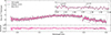 |
Fig. 1. Top panel: Median K-band spectrum for GRAVITY+ (grey) with a median S/N of ≈180. Its best-fit retrieval, including 13CO, is shown in pink, and the retrieval without 13CO is shown in black. The inset shows a zoom-in on the 2.34–2.40 μm region. Bottom panel: Residuals between the data and each model, respectively. The retrieval inflates the error bars in order to find the best-fit model, resulting in residuals not explained by the model. |
3. Methods
3.1. Atmospheric modelling
To characterise β Pic b’s atmosphere, we conducted retrievals using petitRADTRANS (Mollière et al. 2019; Blain et al. 2024; Nasedkin et al. 2024). In our retrievals, a forward model for the spectra was repeatedly evaluated to identify the combinations of the atmospheric parameters that reproduce the observed spectrum. Unlike in a self-consistent modelling approach, as described in Appendix A.4.1, retrievals treat various processes through free parameters and infer their posterior distributions given the data (e.g., Madhusudhan 2018). We used a combination of equilibrium and free chemistry. Most chemical species were interpolated using equilibrium tables, while major radiation absorbing species were freely retrieved. We list the priors of all parameters in Table A.1. The detailed forward model is described in Appendix A.3. Additionally, we cross-correlated template spectra over the 13CO absorption region from 2.34 to 2.40 μm. To construct the 13CO template, we followed Mollière & Snellen (2019), Zhang et al. (2021a) and subtracted the model neglecting 13CO from the best-fit retrieval model. The same subtraction was applied to the data to obtain the 13CO residuals, while the full-model residuals were computed by subtracting the complete model. Prior to cross-correlation, templates were high-pass filtered with a Gaussian kernel (Zhang et al. 2021a), with the kernel width optimised to maximise the signal-to-noise. This balances noise suppression against the over-smoothing of the signal. The residuals were weighted by their measurement uncertainties, ensuring appropriate statistical significance across wavelengths and minimising the contribution of poorly constrained flux points in the cross-correlation function (CCF) signal.
3.2. Variability analysis
A common method to search for variability in time-domain data is via spectral light curves (e.g., Biller et al. 2013). Each spectrum was first cleaned using iterative 3σ clipping to remove instrumental outliers (e.g. bad pixels and residual noise). Our data are affected by strong chromatic variations from fibre coupling (see Fig. A.6 and Sauter et al. 2026); these were removed by dividing each spectrum by the time-averaged mean and fitting a second-order polynomial. Corrected spectra were obtained by dividing the original spectra by this fit, acting as a high-pass filter to remove low-order continuum variations, using a 1D Gaussian kernel of standard deviation σ = 3 pixels along the wavelength axis. As we no longer have access to continuum variability, we analysed variability in the most prominent spectral features, focusing on the 12CO band heads (∼2.29, 2.32, 2.35 μm), which can be affected by chemical instabilities or clouds (Oliveros-Gomez et al. 2026). We restricted our analysis to 2.05–2.355 μm, which still covers all three band heads. Below 2.05 μm, both telluric CO2 and H2O begin to absorb, and beyond 2.35 μm, CH4 and H2O absorb. Additionally, at long wavelengths, thermal background adds noise. We applied generalised Lomb-Scargle (GLS) periodograms (Zechmeister & Kürster 2009) to search for periodicities near the proposed rotational period of ≈8.7 h and its harmonics. The band-head analysis regions span 2.281–2.296 μm, 2.317–2.325 μm, and 2.347–2.352 μm, covering each absorption line and its onset. We then applied sinusoidal fits to the CO band head light curves, with the expected rotation period as an initial guess, to obtain the median periods and amplitudes.
4. Results
4.1. Atmospheric analysis
Our retrieval analysis shows a good fit for our best-fit model to the data, particularly in the 13CO absorption region (see Fig. 1). When comparing our maximal model against our model without 13CO, a flux difference in the 13CO absorption region from 2.34 μm to 2.40 μm is apparent, with the inclusion of 13CO adding additional necessary absorption. Model comparison yields a difference in the Bayesian information criterion (BIC) of ΔBIC ≈ 25, indicating a strong preference for 13CO (Kass & Raftery 1995). We retrieved a 12CO/13CO of 91 (log value of
  ; see Fig. 2), consistent with both the local ISM value of 68 ± 15 (Milam et al. 2005) and the solar value of ∼89 (Wilson & Rood 1994). Our detection is tentatively supported by the cross-correlation function result, which returned a CCF signal of 3.6 (see Fig. A.3). We ran two additional retrievals; one without clouds and one including GPI Y-, J-, and H-band data (Chilcote et al. 2017). Both runs yield an isotopologue ratio consistent with our maximal model (87
 and 91
 , respectively). Although the no-cloud model is preferred (ΔBIC ≈ 73), we adopted the maximal model, as clouds are expected in β Pic b’s atmosphere and the K-band data do not constrain cloud parameters well (Landman et al. 2024). The agreement with the GPI-including retrieval likely reflects the S/N dominance of GRAVITY+; however, we describe these results in Appendix A.5.
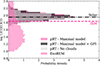 |
Fig. 2. Posterior distributions of log 12CO/13CO for each model, obtained with pRT (solid) and ExoREM (hatched). The distributions are clipped at ±3σ. All three retrieval models show agreement with ISM and solar values, while ExoREM yields a lower ratio, which we disregard due to the decreased fit quality of this self-consistent (less flexible) model. |
4.2. Variability
Fig. 3 shows the first two 12CO band head light curves with their sinusoidal fits. The fits were performed per wavelength, with periods and amplitudes derived from the median and 1σ percentile range of the best-fit parameter distributions. The first and second band heads show well-constrained signals, with periods and amplitudes of 4.4 h and 0.9
 %, and 4.3
 h and 1.92
 %, respectively. These results are both consistent with half the expected rotation period (P/2 ≈ 4.35 h). The third band head (Fig. A.2) yields a similar median period (4.5
 h) and amplitude (1.6
 %) but with highly skewed distributions and extreme outliers, likely due to increased noise beyond 2.35 μm from thermal background and residual tellurics. Combining all three band heads yields 4.4
 h and 1.4
 %, though uncertainties are affected by the third band head. If the variability is dominated by the planet, two interpretations arise. Our 7 h observations do not span the full ≈8.7 h rotation period, yet we find a period consistent with P/2. We have to treat this with caution as VanderPlas (2018) discusses the possibility of periodograms, and therefore sinusoidal fits, picking up low-integer harmonics, over the true signal. Alternatively, the shorter period may reflect atmospheric structure, such as features at opposing longitudes rotating in and out of view. Given the limited temporal coverage and strong telluric and instrumental corrections, confirming a planetary origin requires further analysis, which we will present in future work.
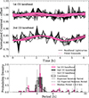 |
Fig. 3. Top panel: Contrast light curves of the first and second CO band head wavelengths with kernel smoothing applied. The pink lines show the fitted sinusoids to each band head. The third band head is shown in Fig. A.2. Bottom panel: Histogram of the distribution of the fitted periods between 0 and 10 h. The probability density for each band head and the total distribution of all band heads are shown. The expected rotation period and its two smaller harmonics are denoted by vertical black lines. The median period is shown in pink and coincides with P/2. |
5. Discussion and conclusion
We presented an analysis of the atmosphere of β Pictoris b using GRAVITY+ data. Our retrievals provide strong statistical evidence for 13CO when compared to the model excluding it, supported by a CCF signal with S/N = 3.6, indicating the absorption feature is well captured. The best-fit model yields  , consistent with ISM and solar values. This is in agreement with upcoming high-resolution results from González Picos et al. (2026, companion paper) using CRIRES+. While our ExoREM analysis does not recover this detection, this likely reflects its resolution-specific issues and the limited flexibility of self-consistent models.
Models of protoplanetary disks show that the 12C/13C ratio could vary across different reservoirs (Woods & Willacy 2009; Lee et al. 2024; Bergin et al. 2024). One possible formation scenario for β Pic b could be accretion from a range of regions and reservoirs that average out, yielding an overall ISM- or solar-like ratio, rather than reflecting a single chemically distinct source. However, this scenario would require specific accretion conditions, balancing contributions of different disk reservoirs, and may be unlikely due to its ‘fine-tuning’ nature. This is further limited by the lack of constraints on the system’s natal disk and the planet’s migration history. González Picos et al. (2025a) propose that the lower 12CO/13CO ratios in younger (metal-rich) M-dwarfs corroborate their later formation. This is because the ISM has become progressively enriched in 13C over time due to galactic chemical evolution (Karakas & Lattanzio 2014). While most Solar System objects (Nomura et al. 2022, and references therein) retain the higher solar ratio (∼89) from 4–5 Gyr ago, β Pic b’s young age (∼23 Myr; Mamajek & Bell 2014) would suggest a value closer to the present-day ISM, such that the derived 12CO/13CO may simply reflect the bulk 12CO/13CO of its host star’s natal cloud. We note, however, that its inferred 12CO/13CO is in agreement with both ISM and solar values, and the margin between these values is small. Nonetheless, we can confidently reject a 13CO enriched 12CO/13CO value. Overall, we conclude that it is still difficult to utilise 13CO as a formation tracer of giant planets, due to the uncertainties that still persist in the models and measurements.
Due to instrumental and telluric noise, extracting β Pic b’s potential variability signal was challenging. However, after applying a novel telluric correction and a second-order polynomial to account for low-order instrumental effects, residual variability persisted in the three 12CO band heads. Preliminarily, we derive a median period of 4.4 h and an amplitude of 1.4
 %. The period is consistent with half the expected rotation period (P/2 ≈4.35 h), even though uncertainties increase with thermal and telluric noise beyond 2.35 μm. The amplitude aligns with the upper limits for early L-type objects Crossfield (2014). While suggestive of planet variability, the signal remains uncertain given the limited temporal baseline and sensitivity to residual systematics. Further observations, such as upcoming JWST work (Zhou et al., in prep.), will be needed to confirm its origin.
Data availability
All reduced data and best fit models are available at https://doi.org/10.5281/zenodo.20608083.
Acknowledgments
This work is based on observations collected at the European Southern Observatory under GRAVITY+ GTO program ID 114.27JS (PI: L. Kreidberg). We would like to acknowledge Nicolas Pourré, who contributed significantly to this project, but has since left astronomy. Additionally, we would like to acknowledge Ewine van Dishoeck for an insightful discussion regarding planet-forming disks and isotopologues. This work benefited from the 2025 Exoplanet Summer Program in the Other Worlds Laboratory (OWL) at the University of California, Santa Cruz, a program funded by the Heising-Simons Foundation and NASA. J.W.X is thankful for support from the Heising-Simons Foundation 51 Pegasi b Fellowship (grant #2025-5887).
References
- Ackerman, A. S., & Marley, M. S. 2001, ApJ, 556, 872 [Google Scholar]
- Allard, N. F., Spiegelman, F., Leininger, T., & Molliere, P. 2019, A&A, 628, A120 [NASA ADS] [CrossRef] [EDP Sciences] [Google Scholar]
- Araújo, A., & Valio, A. 2021, ApJ, 907, L5 [CrossRef] [Google Scholar]
- Baudino, J.-L., Bézard, B., Boccaletti, A., et al. 2015, A&A, 582, A83 [NASA ADS] [CrossRef] [EDP Sciences] [Google Scholar]
- Bergin, E. A., Bosman, A., Teague, R., et al. 2024, ApJ, 965, 147 [NASA ADS] [CrossRef] [Google Scholar]
- Bernath, P. F. 2020, J. Quant. Spectrosc. Radiat. Transfer, 240, 106687 [Google Scholar]
- Biller, B. A., Crossfield, I. J. M., Mancini, L., et al. 2013, ApJ, 778, L10 [Google Scholar]
- Blain, D., Sánchez-López, A., & Mollière, P. 2024, AJ, 167, 179 [NASA ADS] [CrossRef] [Google Scholar]
- Borysow, A. 2002, A&A, 390, 779 [NASA ADS] [CrossRef] [EDP Sciences] [Google Scholar]
- Borysow, A., & Frommhold, L. 1989, ApJ, 341, 549 [NASA ADS] [CrossRef] [Google Scholar]
- Borysow, J., Frommhold, L., & Birnbaum, G. 1988, ApJ, 326, 509 [NASA ADS] [CrossRef] [Google Scholar]
- Borysow, A., Frommhold, L., & Moraldi, M. 1989, ApJ, 336, 495 [NASA ADS] [CrossRef] [Google Scholar]
- Borysow, A., Jorgensen, U. G., & Fu, Y. 2001, J. Quant. Spectrosc. Radiat. Transfer, 68, 235 [NASA ADS] [CrossRef] [Google Scholar]
- Carvalho, A., & Johns-Krull, C. M. 2023, Res. Notes AAS, 7, 91 [Google Scholar]
- Chan, Y. M., & Dalgarno, A. 1965, Proc. Phys. Soc., 85, 227 [NASA ADS] [CrossRef] [Google Scholar]
- Charnay, B., Bézard, B., Baudino, J. L., et al. 2018, ApJ, 854, 172 [Google Scholar]
- Chilcote, J., Pueyo, L., De Rosa, R. J., et al. 2017, AJ, 153, 182 [Google Scholar]
- Crossfield, I. J. M. 2014, A&A, 566, A130 [NASA ADS] [CrossRef] [EDP Sciences] [Google Scholar]
- Dalgarno, A., & Williams, D. A. 1962, ApJ, 136, 690 [NASA ADS] [CrossRef] [Google Scholar]
- de Regt, S., Gandhi, S., Snellen, I. A. G., et al. 2024, A&A, 688, A116 [NASA ADS] [CrossRef] [EDP Sciences] [Google Scholar]
- de Regt, S., Snellen, I. A. G., Allard, N. F., et al. 2025, A&A, 696, A225 [NASA ADS] [CrossRef] [EDP Sciences] [Google Scholar]
- de Regt, S., Snellen, I. A. G., González Picos, D., et al. 2026, A&A, 707, A210 [NASA ADS] [CrossRef] [EDP Sciences] [Google Scholar]
- Gandhi, S., de Regt, S., Snellen, I., et al. 2025, MNRAS, 537, 134 [Google Scholar]
- Gao, P., Thorngren, D. P., Lee, E. K. H., et al. 2020, Nat. Astron., 4, 951 [NASA ADS] [CrossRef] [Google Scholar]
- González Picos, D., Snellen, I. A. G., de Regt, S., et al. 2024, A&A, 689, A212 [NASA ADS] [CrossRef] [EDP Sciences] [Google Scholar]
- González Picos, D., Snellen, I., & de Regt, S. 2025a, Nat. Astron., 9, 1692 [Google Scholar]
- González Picos, D., Snellen, I. A. G., de Regt, S., et al. 2025b, A&A, 693, A298 [NASA ADS] [CrossRef] [EDP Sciences] [Google Scholar]
- González Picos, D., Snellen, I. A. G., Landman, R., et al. 2026, A&A, 711, A87 [NASA ADS] [CrossRef] [EDP Sciences] [Google Scholar]
- Grasser, N., Snellen, I. A. G., de Regt, S., et al. 2025, A&A, 698, A252 [NASA ADS] [CrossRef] [EDP Sciences] [Google Scholar]
- GRAVITY Collaboration (Lacour, S., et al.) 2019, A&A, 623, L11 [NASA ADS] [CrossRef] [EDP Sciences] [Google Scholar]
- GRAVITY Collaboration (Nowak, M., et al.) 2020, A&A, 633, A110 [NASA ADS] [CrossRef] [EDP Sciences] [Google Scholar]
- GRAVITY+ Collaboration (Abuter, R., et al.) 2026, A&A, 707, A115 [Google Scholar]
- Hargreaves, R. J., Gordon, I. E., Rey, M., et al. 2020, ApJS, 247, 55 [NASA ADS] [CrossRef] [Google Scholar]
- Harris, G. J., Tennyson, J., Kaminsky, B. M., Pavlenko, Y. V., & Jones, H. R. A. 2006, MNRAS, 367, 400 [Google Scholar]
- Hauschildt, P. H., & Baron, E. 1999, J. Comput. Appl. Math., 109, 41 [NASA ADS] [CrossRef] [Google Scholar]
- Hauschildt, P. H., Baron, E., & Allard, F. 1997, ApJ, 483, 390 [Google Scholar]
- Hauschildt, P. H., Barman, T., Baron, E., Aufdenberg, J. P., & Schweitzer, A. 2025, A&A, 698, A47 [NASA ADS] [CrossRef] [EDP Sciences] [Google Scholar]
- Karakas, A. I., & Lattanzio, J. C. 2014, PASA, 31, e030 [NASA ADS] [CrossRef] [Google Scholar]
- Kass, R. E., & Raftery, A. E. 1995, J. Am. Stat. Assoc., 90, 773 [Google Scholar]
- Landman, R., Stolker, T., Snellen, I. A. G., et al. 2024, A&A, 682, A48 [NASA ADS] [CrossRef] [EDP Sciences] [Google Scholar]
- Lee, S., Nomura, H., & Furuya, K. 2024, ApJ, 969, 41 [NASA ADS] [CrossRef] [Google Scholar]
- Lei, E., & Mollière, P. 2025, J. Open Source Softw., 10, 7712 [Google Scholar]
- Line, M. R., Teske, J., Burningham, B., Fortney, J. J., & Marley, M. S. 2015, ApJ, 807, 183 [NASA ADS] [CrossRef] [Google Scholar]
- Madhusudhan, N. 2018, in Handbook of Exoplanets, eds. H. J. Deeg, & J. A. Belmonte, 104 [Google Scholar]
- Males, J. R., Close, L. M., Morzinski, K. M., et al. 2014, ApJ, 786, 32 [Google Scholar]
- Mamajek, E. E., & Bell, C. P. M. 2014, MNRAS, 445, 2169 [Google Scholar]
- Marley, M. S., Saumon, D., Cushing, M., et al. 2012, ApJ, 754, 135 [Google Scholar]
- McCarthy, A. M., Vos, J. M., Muirhead, P. S., et al. 2025, ApJ, 981, L22 [Google Scholar]
- Milam, S. N., Savage, C., Brewster, M. A., Ziurys, L. M., & Wyckoff, S. 2005, ApJ, 634, 1126 [Google Scholar]
- Mollière, P., & Snellen, I. A. G. 2019, A&A, 622, A139 [NASA ADS] [CrossRef] [EDP Sciences] [Google Scholar]
- Mollière, P., Wardenier, J. P., van Boekel, R., et al. 2019, A&A, 627, A67 [Google Scholar]
- Mollière, P., Molyarova, T., Bitsch, B., et al. 2022, ApJ, 934, 74 [CrossRef] [Google Scholar]
- Mollière, P., Kühnle, H., Matthews, E. C., et al. 2025, A&A, 703, A79 [NASA ADS] [CrossRef] [EDP Sciences] [Google Scholar]
- Morley, C. V., Mukherjee, S., Marley, M. S., et al. 2024, ApJ, 975, 59 [NASA ADS] [CrossRef] [Google Scholar]
- Nasedkin, E., Mollière, P., & Blain, D. 2024, J. Open Source Softw., 9, 5875 [CrossRef] [Google Scholar]
- Nomura, H., Furuya, K., Cordiner, M. A., et al. 2022, arXiv e-prints [arXiv:2203.10863] [Google Scholar]
- Öberg, K. I., Murray-Clay, R., & Bergin, E. A. 2011, ApJ, 743, L16 [Google Scholar]
- Oliveros-Gomez, N., Manjavacas, E., Karalidi, T., et al. 2026, ApJ, 997, 136 [Google Scholar]
- Polyansky, O. L., Kyuberis, A. A., Zobov, N. F., et al. 2018, MNRAS, 480, 2597 [NASA ADS] [CrossRef] [Google Scholar]
- Radigan, J. 2014, ApJ, 797, 120 [NASA ADS] [CrossRef] [Google Scholar]
- Ravet, M., Bonnefoy, M., Chauvin, G., et al. 2025, A&A, 704, A325 [NASA ADS] [CrossRef] [EDP Sciences] [Google Scholar]
- Reggiani, H., Galarza, J. Y., Schlaufman, K. C., et al. 2024, AJ, 167, 45 [Google Scholar]
- Rothman, L. S., Gordon, I. E., Barber, R. J., et al. 2010, J. Quant. Spectrosc. Radiat. Transfer, 111, 2139 [NASA ADS] [CrossRef] [Google Scholar]
- Rothman, L. S., Gordon, I. E., Babikov, Y., et al. 2013, J. Quant. Spectrosc. Radiat. Transfer, 130, 4 [Google Scholar]
- Royer, F., Zorec, J., & Gómez, A. E. 2004, IAU Symp., 224, 109 [Google Scholar]
- Ruffio, J.-B., Macintosh, B., Konopacky, Q. M., et al. 2019, AJ, 158, 200 [Google Scholar]
- Ruffio, J.-B., Xuan, J. W., Chachan, Y., et al. 2026, Nat. Astron., 10, 511 [Google Scholar]
- Sauter, J. R., von Stauffenberg, A., Bourdarot, G., et al. 2026, A&A, 708, A367 [NASA ADS] [CrossRef] [EDP Sciences] [Google Scholar]
- Sousa-Silva, C., Al-Refaie, A. F., Tennyson, J., & Yurchenko, S. N. 2015, MNRAS, 446, 2337 [Google Scholar]
- Swastik, C., Banyal, R. K., Narang, M., et al. 2021, AJ, 161, 114 [Google Scholar]
- VanderPlas, J. T. 2018, ApJS, 236, 16 [Google Scholar]
- Wilson, T. L., & Rood, R. 1994, ARA&A, 32, 191 [Google Scholar]
- Woods, P. M., & Willacy, K. 2009, ApJ, 693, 1360 [Google Scholar]
- Xuan, J. W., Ruffio, J.-B., Chachan, Y., et al. 2026, ApJ, 1000, 27 [Google Scholar]
- Zechmeister, M., & Kürster, M. 2009, A&A, 496, 577 [CrossRef] [EDP Sciences] [Google Scholar]
- Zhang, Y., Snellen, I. A. G., Bohn, A. J., et al. 2021a, Nature, 595, 370 [NASA ADS] [CrossRef] [Google Scholar]
- Zhang, Y., Snellen, I. A. G., & Mollière, P. 2021b, A&A, 656, A76 [NASA ADS] [CrossRef] [EDP Sciences] [Google Scholar]
- Zhang, Z., Mollière, P., Hawkins, K., et al. 2023, AJ, 166, 198 [NASA ADS] [CrossRef] [Google Scholar]
- Zhang, Y., González Picos, D., de Regt, S., et al. 2024, AJ, 168, 246 [NASA ADS] [CrossRef] [Google Scholar]
- Zhang, Z., Mollière, P., Fortney, J. J., & Marley, M. S. 2025, AJ, 170, 64 [Google Scholar]
Appendix A: Additional figures and tables
A.1. Telluric correction
The 13CO signal and the variability signal are both highly sensitive and can be significantly affected by telluric contamination in our observations. If not properly corrected, these signals may be indistinguishable from the planetary signals. The current method for estimating the stellar coherent fluxes during the planet observations involves averaging the absolute coherent fluxes of the bracketing on-star observations. However, this does not take into account the airmass trend, which will be larger towards the start and the end of the night, which, according to the Beer–Lambert law, traces the telluric transmissivity. To address this, we employed a novel telluric correction technique first introduced by Sauter et al. (2026), for the same observations. The correction was performed using a linear interpolation between the two adjacent stellar observations as follows:
 (A.1)
(A.1)
where ΓStar 1 and ΓStar 2 are the coherent flux values of the on-star observations before and after a planet observation. Similarly AMStar 1 and AMStar 2 denote the airmass values for the on-star observations and AMplanet for the planet observations. Lastly, w defines a weighting factor that accounts for small changes in airmass to avoid numerical instabilities:
 (A.2)
(A.2)
Here δ was empirically chosen to be 0.03. It has to be noted that, due to no star observations being taken after the last two planet observations, this data reduction only utilises 36 of the on-planet observations instead of the 38 available ones.
A.2. Mean averaging spectra
As our observations span ≈7 hrs with multiple epoch spectra, we combined these to boost our S/N for the retrieval analysis. Prior to averaging the spectra, outlier removal was done through sigma clipping using a 4σ tolerance. Assuming a normal distribution of the errors, this would include 99.9937% of the data. The mean flux in each wavelength bin was then computed through element-wise mean averaging, which was done by averaging all flux values from all spectra that fall inside that bin, not including the outliers:
 (A.3)
(A.3)
where N is the total number of spectra, i the spectral index, and S the flux value for a specific wavelength bin. The corresponding mean covariance matrix is computed using the following equation:
![Mathematical equation: $$ \begin{aligned} \mathrm{Cov}\left[ \overline{x} \right]=\frac{1}{N^2}\sum ^N_{i = 1}\mathrm{Cov}\left[ x_i \right] =\frac{1}{N^2}\sum ^N_{i = 1}\Sigma _i. \end{aligned} $$](/articles/aa/full_html/2026/07/aa60275-26/aa60275-26-eq22.gif) (A.4)
(A.4)
Here it has to be noted that the 1/N division is applied with awareness of the outlier removal. After sigma clipping, the number of contributing flux values can differ between wavelength bins. For a given bin, the average was therefore computed using only the remaining (non-clipped) samples. This way, we were able to maintain the full wavelength range while still removing spurious data points, which results in those bins having slightly overestimated uncertainties compared to bins that had no outliers removed.
A.3. Retrieval forward model
We defined our forward model as follows: The pressure-temperature (P-T) structure was based on Zhang et al. (2025). This is a P-T parametrisation first introduced in Zhang et al. (2023), where the atmosphere is divided into ten logarithmically spaced pressure layers, going from 103 to 10−6, and then between these points is interpolated quadratically. This model therefore introduces eleven new free parameters. Ten of these represent the temperature gradient dlnT/dlnP at the pressure layers, and one a reference temperature (Tref) at a given pressure. For the seven gradients positioned at highest pressures, the priors are based on the 1-σ confidence values of the distributions derived from the self-consistent P-T profiles of SONORA DIAMONDBACK (Morley et al. 2024). As the profiles in Morley et al. (2024) do not reach upper atmosphere pressures of 10−4, the final three layers extending to 10−6 can vary freely, as described in Mollière et al. (2025). As clouds have been shown to have an impact on the spectrum of β Pic b (GRAVITY Collaboration 2020; Ravet et al. 2025), we kept scattering on for our retrievals and attempted to retrieve cloud properties implemented in pRT based on Ackerman & Marley (2001), with the clouds being parametrised the same way as in Mollière et al. (2025).
The chemical abundances were mostly interpolated using chemical equilibrium tables already included in pRT, calculated with easyCHEM (Lei & Mollière 2025), especially for any species we expected to be only background contributors. For these species, we retrieved the atmospheric C/O ratio and metallicity. However, for the species we expected to majorly impact the shape and features of the spectrum, we separately retrieved the mass fractions. This included CO2,13CO, 12CO, H2O, and CH4, which are most relevant in the K-band. The values for the atmospheric metallicity and C/O ratio were then calculated using the absorber mass fractions determined from chemical equilibrium abundances and the freely retrieved abundances, with resulting values shown in Table A.1.
Piors and mean posteriors with their 1σ uncertainties derived from the retrievals with petitRADTRANS. The value 𝒩 defines Gaussian priors, while 𝒰 signifies uniform priors.
At a resolution of 4000, we had to factor in rotational broadening of the planet’s atmospheric lines for our model spectra. Here we used the code described in Carvalho & Johns-Krull (2023). We assumed the default value of 0.6 for limb darkening and split up our planet in 10 radial bins and 100 azimuthal bins. While work is being done to explore differential rotation in brown dwarfs and exoplanets (e.g. Araújo & Valio 2021), we kept the differential rotation at 0, as it has not been measured for β Pic b so far, and the inclination of the planet remains unclear.
The sources of the included opacities are the following: the collision-induced absorption opacities H2−H2 (Borysow et al. 2001; Borysow 2002) and H2−He (Borysow et al. 1988, 1989; Borysow & Frommhold 1989). The Rayleigh scattering opacities H2 (Dalgarno & Williams 1962) and He (Chan & Dalgarno 1965). The line opacities H2O (Polyansky et al. 2018), CH4 (Hargreaves et al. 2020), CO2 (Rothman et al. 2010), 12CO (Rothman et al. 2010), 13CO (Rothman et al. 2013), Na (Allard et al. 2019), K (line profiles by N. Allard, see Mollière et al. 2019), TiO (line lists by B. Plez, see Mollière et al. 2019), FeH (Bernath 2020), NH3 (Rothman et al. 2013), PH3 (Sousa-Silva et al. 2015), HCN (Harris et al. 2006), H2S (Rothman et al. 2013).
In order to account for possible model inaccuracies and underestimated observational noise, we introduced uncertainty scaling to our retrieval method. In our retrievals, we added this scaling to our data set, as a free parameter. Here we followed the procedure described in Line et al. (2015), whereby the flux uncertainty σ is scaled as following:
![Mathematical equation: $$ \begin{aligned} \sigma _{\mathrm{scaled}} = [\sigma ^2(\lambda )+10^b]^{1/2}. \end{aligned} $$](/articles/aa/full_html/2026/07/aa60275-26/aa60275-26-eq60.gif) (A.5)
(A.5)
This was done for the diagonal elements of the covariance matrices. If this scaling was not applied and underestimations are present from the data reduction process, the retrieval would become overly confident in the fit, and return narrower parameter distribution widths than they should be. Therefore, we freely retrieved the b parameter to estimate the scaled uncertainty. The priors for this uncertainty scaling were taken from Line et al. (2015).
A.4. Self consistent modelling
A.4.1. Method
To independently analyse our dataset, we also employed the self-consistent modelling grid ExoREM with ForMoSA2, as was done in Ravet et al. (2025). By adding a self-consistent model to our analysis, especially because of the limited spectral range (GRAVITY+ data in K-band dominates even if GPI is added in the free retrievals), we may be able to more accurately constrain bulk parameters such as effective temperature. We could also test whether self-consistent models are flexible enough to detect trace species such as 13CO. ExoREM is a radiative-convective equilibrium code with a grid specifically aimed to model young giant planetary mass companions (Baudino et al. 2015), with the bulk parameters spanning 400K ≤ Teff ≤ 2000K, 3.0 ≤ logg ≤ 5.0, −0.5 ≤ [M/H] ≤ 2.0, 0.10 ≤ C/O ≤ 0.80 and a custom grid for 13CO. However, we have restricted these priors to a suitable range for our analysis and added relevant parameters, as described in Table A.2. ExoREM also incorporates both iron and silicate clouds, as implemented in Charnay et al. (2018). This is particularly relevant as both GRAVITY Collaboration (2020) and Ravet et al. (2025) found evidence of clouds in the atmosphere of β Pic b, and silicate species are expected to condense in this temperature regime (Gao et al. 2020). Clouds are treated with a simplified self-consistent parametrisation within this framework, which in this case means that it is driven by only the fastest micro-physical processes. This includes the vertical cloud distribution being computed by balancing sedimentation against vertical mixing, using an eddy diffusion coefficient Kzz, which also allows for disequilibrium chemistry. Due to the medium resolution of the data, we also included rotational broadening in the analysis, where we fixed v sin i to the value found in Landman et al. (2024) (19.9 km/s). Similarly to the uncertainty scaling in the retrievals, we could introduce a global scaling parameter (s) in ForMoSA following Ruffio et al. (2019). For this, the covariance was rescaled from C to s2C. Rather than fitting for s explicitly, we marginalised s with respect to the likelihood.
Priors and mean posteriors with their 1σ uncertainties using self-consistent modelling with ExoREM
A.4.2. Results
The self-consistent best-fit shows slightly more spread residuals in comparison to the retrieval best-fit, especially in the 13CO absorption region. When inspecting this region more closely, in the middle panel of Fig. A.4, we can see that ExoREM is not flexible enough to accurately fit the depths of the lines in this region. This could be affected by the available ExoREM spectra are generated at R ∼10, 000 − 8, 000 in the K band but are only Nyquist sampled at R ∼5, 000 − 4, 000, which would in turn reduce the effective model resolution beyond ∼2.3 μm relative to GRAVITY. We do attempt to oversample the ExoREM spectra by interpolating them to the more finely spaced wavelength grid of the observations, which does pose risks but preserves the GRAVITY+ resolution. However, this could somewhat limit the ability to capture the line shapes of 12CO and 13CO and affect the signal in the cross-correlation function. Nonetheless we do get a constraint for 13CO, with a 12CO/13CO ratio of  , as shown in Figure 2, which would indicate a strongly enriched 13CO abundance. Given that the ExoREM posterior distribution shows a long tail, the models do not accurately reproduce the CO line shapes and show no significant cross-correlation peak at 0,km,s−1, we do not consider the inferred 12CO/13CO ratio to be a robust constraint. Additionally, in Fig. A.4 it shows a small underestimation of flux at the bluest wavelengths, where H2O absorbs. This may indicate a lack of flexibility of the grid modelling approach, or too weak removal of tellurics, as less flux is removed than should be according to self-consistent physics.
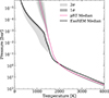 |
Fig. A.1. Displays median pressure-temperature profiles from the two best-fit models using petitRADTRANS (pink) and ExoREM (black). The grey shading represents the 1- and 2σ uncertainty envelopes for each model. |
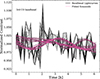 |
Fig. A.2. Contrast light curves of the third CO band-head wavelengths with kernel smoothing applied. The pink lines show the fitted sinusoids to the light curves. The first and second band heads are shown in Figure 3. |
A.5. Adding GPI data
In our retrieval analysis, we ran our retrieval model on the Y-, J-, and H-band GPI data from Chilcote et al. (2017) together with our GRAVITY+ data, in addition to the model presented in the main text. As noted by GRAVITY Collaboration (2020), while the GRAVITY K-band data are important for constraining the C/O ratio, the GPI Y-, J-, and H-band data are needed to better constrain log, g. Therefore, the motivation for including the additional short-wavelength spectral information was to better constrain bulk parameters, and since there is a well-established correlation between gravity and clouds (Marley et al. 2012), we hoped this might also help constrain the cloud parameters. Improvement in constraining other atmospheric parameters thereby could possibly improve the detection of 13CO or the constraint of the 12CO/13CO ratio. The best fit model is shown in Figure A.5, where it is apparent that the quality of the fit is worse for the GPI data, which is likely caused by the GRAVITY+ data dominating the fit due to its significantly higher S/N and number of data points. This is especially shown in the H-band where the retrieval fits a much stronger triangular shape than indicated by the observed spectrum. Including these data sets, however, does appear to affect the values for log, g, C/O, and metallicity (see Table A.3), pushing all these values higher. This results in a significantly super-solar C/O ratio and a super-solar metallicity. On the other hand, the cloud parameters remain unconstrained, while the retrieved 12CO/13CO ratio remains fully consistent with the GRAVITY-only results. This result might originate from the poor reproduction of the GPI spectra, meaning the retrieval cannot meaningfully exploit the additional wavelength coverage to constrain the cloud parameters, despite the GPI data nominally covering a regime where the degeneracy between log, g and cloud parameters might otherwise be broken. The changes in C/O and metallicity, while statistically significant, should be interpreted with caution; if the model is unable to adequately fit the GPI data, the resulting posteriors for these parameters may reflect the retrieval compensating for systematic residuals rather than a genuine improvement in constraint. This is supported by the 12CO/13CO ratio that appears to be almost exclusively determined by the high-resolution CO features in the GRAVITY+ K-band data, which seem unaffected by the inclusion of the GPI data. We therefore consider the GRAVITY-only values of C/O and metallicity to be more reliable, and treat the GPI retrieval results primarily as a consistency check rather than an independent constraint.
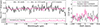 |
Fig. A.3. Top panel: Cross-correlation templates created from the retrieved models. The observational residuals, shown in black, are the data and the best-fit model, with 13CO turned off, subtracted. In pink, the best-fit model is subtracted from that same model but with 13CO manually turned off, yielding the 13CO template. The dashed grey line shows the residuals when subtracting the full model from the data. Bottom panel: Observational uncertainties, by which we weighted the residuals. Right panel: Cross-correlation function for each of the residuals with the 13CO template. The CCF between the 13CO residuals remaining in the data and the 13CO template is shown in pink, while the dot-dashed black line shows the cross-correlation between the full model residuals and the 13CO template. The autocorrelation of the 13CO signal is shown with the dashed light-pink line. |
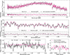 |
Fig. A.4. Top panel: Comparison between the retrieval (pink) and the self-consistent model (black), as well as their respective residuals to the data. Middle panel: Zoom-in on the active 13CO absorption region between 2.34 μm and 2.4 μm. Bottom panel: Cross-correlation templates for the self-consistent model similar to Fig. A.3 together with the cross-correlation function. |
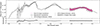 |
Fig. A.5. Top panel: Best-fit retrieval model for the GPI and GRAVITY+ data. The grey squares and grey triangles show the GPI Y-, J-, and H-band data from Chilcote et al. (2017), respectively, and the grey circles show the GRAVITY+ mean K-band data from this work, all with their respective uncertainties. The black line shows the best-fit model convolved to the GPI spectral resolution of R∼70, and the pink line shows the corresponding high-resolution model. For clarity, the high-resolution model is shown only in the K band. Bottom panel: Respective residuals between the model and datasets. |
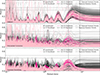 |
Fig. A.6. GLS periodograms of individual wavelength contrast light curves. In each of the panels, the light pink, dark pink, and black highlighted lines are the first, second, and third 12CO band heads, respectively. The horizontal grey lines indicate the 1%, 5%, and 10% false alarm probabilities. The vertical black lines indicate the expected rotation period at 8.7 hrs and its first integer harmonic at 4.35 hrs. Top: Uncorrected periodogram, with all wavelengths significantly affected by systematic effects caused by the fibre coupling. Middle: Periodogram after the polynomial correction. Bottom: Gaussian smoothing added to the periodogram to highlight the strong periodic signals. |
Mean posterior values with their 1σ uncertainties for bulk atmospheric parameters derived from the retrievals using petitRADTRANS for both the GRAVITY+ only models and those including GPI data (Chilcote et al. 2017). These include the derived 12CO/13CO ratio and effective temperature.
All Tables
Piors and mean posteriors with their 1σ uncertainties derived from the retrievals with petitRADTRANS. The value 𝒩 defines Gaussian priors, while 𝒰 signifies uniform priors.
Priors and mean posteriors with their 1σ uncertainties using self-consistent modelling with ExoREM
Mean posterior values with their 1σ uncertainties for bulk atmospheric parameters derived from the retrievals using petitRADTRANS for both the GRAVITY+ only models and those including GPI data (Chilcote et al. 2017). These include the derived 12CO/13CO ratio and effective temperature.
All Figures
|
Fig. 1. Top panel: Median K-band spectrum for GRAVITY+ (grey) with a median S/N of ≈180. Its best-fit retrieval, including 13CO, is shown in pink, and the retrieval without 13CO is shown in black. The inset shows a zoom-in on the 2.34–2.40 μm region. Bottom panel: Residuals between the data and each model, respectively. The retrieval inflates the error bars in order to find the best-fit model, resulting in residuals not explained by the model. |
| In the text | |
|
Fig. 2. Posterior distributions of log 12CO/13CO for each model, obtained with pRT (solid) and ExoREM (hatched). The distributions are clipped at ±3σ. All three retrieval models show agreement with ISM and solar values, while ExoREM yields a lower ratio, which we disregard due to the decreased fit quality of this self-consistent (less flexible) model. |
| In the text | |
|
Fig. 3. Top panel: Contrast light curves of the first and second CO band head wavelengths with kernel smoothing applied. The pink lines show the fitted sinusoids to each band head. The third band head is shown in Fig. A.2. Bottom panel: Histogram of the distribution of the fitted periods between 0 and 10 h. The probability density for each band head and the total distribution of all band heads are shown. The expected rotation period and its two smaller harmonics are denoted by vertical black lines. The median period is shown in pink and coincides with P/2. |
| In the text | |
|
Fig. A.1. Displays median pressure-temperature profiles from the two best-fit models using petitRADTRANS (pink) and ExoREM (black). The grey shading represents the 1- and 2σ uncertainty envelopes for each model. |
| In the text | |
|
Fig. A.2. Contrast light curves of the third CO band-head wavelengths with kernel smoothing applied. The pink lines show the fitted sinusoids to the light curves. The first and second band heads are shown in Figure 3. |
| In the text | |
|
Fig. A.3. Top panel: Cross-correlation templates created from the retrieved models. The observational residuals, shown in black, are the data and the best-fit model, with 13CO turned off, subtracted. In pink, the best-fit model is subtracted from that same model but with 13CO manually turned off, yielding the 13CO template. The dashed grey line shows the residuals when subtracting the full model from the data. Bottom panel: Observational uncertainties, by which we weighted the residuals. Right panel: Cross-correlation function for each of the residuals with the 13CO template. The CCF between the 13CO residuals remaining in the data and the 13CO template is shown in pink, while the dot-dashed black line shows the cross-correlation between the full model residuals and the 13CO template. The autocorrelation of the 13CO signal is shown with the dashed light-pink line. |
| In the text | |
|
Fig. A.4. Top panel: Comparison between the retrieval (pink) and the self-consistent model (black), as well as their respective residuals to the data. Middle panel: Zoom-in on the active 13CO absorption region between 2.34 μm and 2.4 μm. Bottom panel: Cross-correlation templates for the self-consistent model similar to Fig. A.3 together with the cross-correlation function. |
| In the text | |
|
Fig. A.5. Top panel: Best-fit retrieval model for the GPI and GRAVITY+ data. The grey squares and grey triangles show the GPI Y-, J-, and H-band data from Chilcote et al. (2017), respectively, and the grey circles show the GRAVITY+ mean K-band data from this work, all with their respective uncertainties. The black line shows the best-fit model convolved to the GPI spectral resolution of R∼70, and the pink line shows the corresponding high-resolution model. For clarity, the high-resolution model is shown only in the K band. Bottom panel: Respective residuals between the model and datasets. |
| In the text | |
|
Fig. A.6. GLS periodograms of individual wavelength contrast light curves. In each of the panels, the light pink, dark pink, and black highlighted lines are the first, second, and third 12CO band heads, respectively. The horizontal grey lines indicate the 1%, 5%, and 10% false alarm probabilities. The vertical black lines indicate the expected rotation period at 8.7 hrs and its first integer harmonic at 4.35 hrs. Top: Uncorrected periodogram, with all wavelengths significantly affected by systematic effects caused by the fibre coupling. Middle: Periodogram after the polynomial correction. Bottom: Gaussian smoothing added to the periodogram to highlight the strong periodic signals. |
| In the text | |
Current usage metrics show cumulative count of Article Views (full-text article views including HTML views, PDF and ePub downloads, according to the available data) and Abstracts Views on Vision4Press platform.
Data correspond to usage on the plateform after 2015. The current usage metrics is available 48-96 hours after online publication and is updated daily on week days.
Initial download of the metrics may take a while.