


| Issue |
A&A
Volume 711, July 2026
|
|
|---|---|---|
| Article Number | A297 | |
| Number of page(s) | 22 | |
| Section | Stellar structure and evolution | |
| DOI | https://doi.org/10.1051/0004-6361/202660047 | |
| Published online | 24 July 2026 | |
Configuration of the ξ Tau system constrained by multi-technique observations
1
Charles University, Faculty of Mathematics and Physics, Institute of Astronomy, V Holešovičkách 2, CZ-18000 Prague, Czech Republic
2
High Point University, Department of Physics, One University Way, High Point, NC 27268, USA
3
University of Zagreb, Faculty of Geodesy, Hvar Observatory, Kačićeva 26, 10000 Zagreb, Croatia
4
Observatoire de Paris, LIRA, Université PSL, CNRS, Sorbonne Université, Université Paris Cité, CY Cergy Paris Université, 92190 Meudon, France
5
Technical University of Denmark, DTU Space, Elektrovej 327, Kgs. Lyngby 2800, Denmark
6
Universität Graz, Institut für Physik, Universitätsplatz 3, 8010 Graz, Austria
7
Universität Wien, Institut für Astrophysik, Türkenschanzstrasse 17, 1180 Vienna, Austria
8
University of British Columbia, Department of Physics and Astronomy, 6224 Agricultural Road, Vancouver, BC V6T 1Z1, Canada
9
Université Côte d’Azur, Observatoire de la Côte d’Azur, CNRS, Laboratoire Lagrange, Parc Valrose, 06108 Nice, France
★ Corresponding author: This email address is being protected from spambots. You need JavaScript enabled to view it.
Received:
24
March
2026
Accepted:
21
May
2026
Abstract
Context.ξ Tau is one of the most compact multiple stellar systems, which is sufficiently close (67 pc) to be constrained by all kinds of observations.
Aims. To better constrain the current configuration of ξ Tau and to study its temporal evolution, we aim to utilize new observational data: (i) publicly available photometry from TESS and astrometry from WDS; and (ii) our own photometry from the MOST spacecraft and spectroscopy from the CTIO observatory.
Methods. As a prerequisite, we accurately described the CTIO/CHIRON echelle instrument so that interpolation of the blaze function over the Balmer lines (Hα, Hβ) would allow us to rectify the wings with minimal systematics. We then used our previous model of ξ Tau and constrained it by the new data. At the same time, we improved our dynamical model by accounting not only for mutual, N-body perturbations, but also for relativistic effects, oblateness, and tides. We optimized grids of models, showing χ2 contributions from 11 different types of observations (astrometry, radial velocities, transit-timing variations, light curves, interferometric visibility, closure phase, etc.). This allowed us to find the global, best-fit solution, keeping track of possible ‘tension’ among the different data.
Results. Given the hierarchical architecture of ξ Tau, ((Aa+Ab)+B)+C, we detected the orbital evolution on all timescales. Oscillations of periods, P, occur on the shortest orbital timescales (P1, P2); the variation of eccentricity, e1, is from 0 to 0.008, and that of e2 is from 0.202 to 0.207. Oscillations of projected i, Ω are coupled and occur on the secular timescale of about 7000 d. The inclination, i1, of the inner, eclipsing pair (Aa+Ab) changes from 86.1° to 87.1°, which is clearly manifested in eclipse depths. There is also a long-term trend due to the outer orbit (P3 ≐ 18900 d), with a perihelion passage (a ‘bump’) of component C, which is manifested in radial velocities. The mutual inclinations among the three orbital planes, ≃0.5° and 71°, are very different. Long-term stability is ensured by suppressing Kozai oscillations due to the fast precession rate ω˙. The best model requires tidal dissipation in the inner binary (with the time lag of ∼100 s) and five components, where component C is a binary (Ca+Cb).
Conclusions. Although the masses of the three components (2.27, 2.15, 3.78 M⊙) are now constrained to within 1%, the suspected binary (Ca+Cb), offset by 600 mas, should be better characterized. A key question remains whether this bright stellar system contains additional dwarf or exoplanetary components with low masses. Continuing monitoring of ξ Tau is highly desirable.
Key words: binaries: eclipsing / stars: fundamental parameters / stars: individual: ξ Tau
© The Authors 2026
 Open Access article, published by EDP Sciences, under the terms of the Creative Commons Attribution License (https://creativecommons.org/licenses/by/4.0), which permits unrestricted use, distribution, and reproduction in any medium, provided the original work is properly cited.
This article is published in open access under the Subscribe to Open model. This email address is being protected from spambots. You need JavaScript enabled to view it. to support open access publication.
1. Introduction
Triple, quadruple, or quintuple stellar systems are not just ‘more complicated binaries’ (Tokovinin & Moe 2020; Tokovinin 2021; Borkovits et al. 2020; Borkovits 2022). They were not assembled randomly, but their varying architectures and occurrences (2+1, 3+1, 2+2, 3+2, etc.) suggest several evolutionary processes, for example, migration, Kozai cycles, tidal friction, magnetic friction, envelope expansion, mass transfer, close encounters, or ejections.
Less complicated binaries form a foundation of the universal distance scale (Pietrzyński et al. 2013, 2019; Gallenne et al. 2023), provided their properties were measured with percentage-level precision. Multiples allowed us to achieve even higher precision due to additional dynamical constraints (Borkovits 2022; Brož et al. 2025). Two or more orbits might also serve as an additional verification.
The ξ Tau system is composed of four components (Aa, Ab, B, C). From a Solar-System perspective, the inner eclipsing binary has a semi-major axis of only 0.11 au, the third component is similar to the Earth (∼1.1 au), and the fourth component is similar to Neptune (29 au); the total mass is over 9 M⊙.
In our previous work (Nemravová et al. 2016), we used space-based photometry from the Microvariability and Oscillations of Stars Satellite (MOST) (Walker et al. 2003), which allowed a clear detection of mutual perturbations; for example, the eclipse-timing variations (ETVs) exhibit an amplitude of about half an hour. In this work, we aim to use space-based photometry from the Transiting Exoplanet Survey Satellite (TESS) (Ricker et al. 2015) and an additional set of MOST observations from 2017, supplemented by ground-based spectroscopy from Cerro Tololo Inter-American Observatory (CTIO) (Tokovinin et al. 2013). Consequently, the high-accuracy observations extend over a substantially longer time span. Their analysis should allow a much better characterization of the system parameters, including evidence of the evolution of ξ Tau orbital architecture on various timescales (from days to decades).
A related scientific question is whether or not this stellar system also contains exoplanets. More than 800 exoplanets are already known in binaries (Thebault & Haghighipour 2015; Thebault & Bonanni 2025). More than 30 are circumbinary, where a secondary is commonly located at 0.1 au and an exoplanet at ∼0.5 au, which is close to the stability limit (Holman & Wiegert 1999). This rough statistics is biased, though, especially for O or B stars, which are much brighter than exoplanets. One should keep this in mind when studying bright stellar systems.
Hereinafter, we describe only new observations of ξ Tau (Sect. 2), since old observations were described in Nemravová et al. (2016). Subsequently, we describe models of ξ Tau of various complexities, the reference one (Sect. 3.1), the interferometric one (Sect. 3.2), the all-data model (Sect. 3.3), the model with tides (Sect. 3.4), and the model with five components (Sect. 3.5). The temporal evolution of the ξ Tau system is discussed in Sect. 4 and additional aspects (parallax, oscillations) are detailed in Sect. 5. The conclusions are presented in Sect. 6.
2. New observations
2.1. Hvar photometry
Systematic photometry was collected at the Hvar Observatory with the 0.65-m reflector and photoelectric photometer, initially in UBV bands (2007–2013) and later in UBVR bands (2013–2025). After a recent revision of 52 years of Hvar observations (Božić et al. 2026), all-sky magnitudes of all comparison stars were derived relatively to the Johnson standards and all observations were carefully transformed to the standard Johnson UBV system (Harmanec et al. 1994). The latest reduction includes also temporal variation of the extinction coefficients in the course of night. The Hvar mean values for comparison stars, 4 Tau = HD 21686, and 6 Tau = HD 21933, which were added to the differential magnitudes, are V = 5.150, B − V = −0.045, U − B = −0.093, V − R = −0.016; V = 5.774, B − V = −0.076, U − B = −0.300, V − R = −0.025.
We note that the transparency curve of the R filter closely corresponds to that of the standard Cousins R filter. However, because we were not able to find enough northern bright standard stars with the Cousins Rc values, we derived robust mean values of Johnson V − R indices from Johnson et al. (1966) and reduced our observations to the Johnson R magnitude.
2.2. MOST photometry
Broadband photometry obtained by the MOST satellite (Walker et al. 2003) consists of two separate sets of observations. Back in 2012, J. Nemravová and P. Harmanec submitted a successful application for observations of ξ Tau to the MOST allocation committee, and continuous light curve observations were indeed obtained. These observations were published in Nemravová et al. (2016), along with the discovery of low-amplitude photometric oscillations on the time scale of about 0.4 d. We use these data also here.
The second data set was obtained on a commercial basis at the end of 2017 and represents the last set of scientifically usable MOST data before the communication with the satellite was lost forever. The data were downloaded at the Vienna tracking station and their initial reduction was carried out by T. Kallinger.
2.3. TESS photometry
Photometry obtained by the TESS satellite (Ricker et al. 2015) was also included. TESS records red optical light, with a wide bandpass spanning roughly 600−1000 nm centered on the traditional Cousins I band. TESS observed ξ Tau in six sectors (31, 42, 43, 44, 70, 71). Basic reductions and cleaning were performed by Jon Labadie-Bartz. Light curves were extracted from the full frame images with the Lightkurve package (Cardoso et al. 2018) using simple aperture photometry, including the saturated columns and their ‘spillover’ pixel end caps, and the non-saturated halo pixels, as is standard for moderately saturated bright stars. The observing cadence was ten minutes (sectors 31, 42, 43, 44) and 200 seconds (sectors 70, 71). Background subtraction was used as the preferred detrending method. ξ Tau is fairly isolated on the sky and so blending from neighboring stars did not contribute to the observed signals.
The series of light curves represents the key observational constraint, because the exact epochs of eclipses are sensitive to the perturbations by the component B. These include both the geometric effects due to finite speed of light and variations in position of the eclipsed star with respect to the observer (usually termed light-time effect), and variations in the orbital elements of the eclipsing binary due to the gravitational perturbations by the component B (often termed physical timing variations).
2.4. CTIO/CHIRON spectroscopy
The CHIRON instrument (Tokovinin et al. 2013) at the CTIO 1.5-m telescope is an echelle spectrograph. Its resolution is R = 79000 (higher resolution was not used), spectral range 410 to 890 nm, and efficiency at least 6%. It is equipped with the back-illuminated detector CCD231-84 Teledyne E2v, with 4094 × 4112 pixels and gain of η = 1.3 adu/e−. We performed a standard reduction of spectra by applying a dark frame and a flat field and by calibrating the wavelength scale with a ThAr lamp spectrum. For a detailed description of rectification, see Appendix A.
In the course of observational campaign, we obtained 277 spectra of ξ Tau (excluding defective ones). The spectral range was limited to 450 to 890 nm, divided into 62 orders (including some overlaps and gaps), with 801 pixels per order. The exposure time was 60 s, the peak signal reaching S = 160000 adu, resulting in the signal-to-noise ratio  . We observed sequences of five spectra. The total time span was 129 days, from Sep. 15 2021 to Jan. 21 2022, covering the short orbit (Aa+Ab) 18 times and about 90% of the long orbit ((Aa+Ab)+B).
2.5. Gaia parallax
The parallax in the Gaia EDR3/DR3 release (Bailer-Jones et al. 2021; Vallenari et al. 2023) is π = (16.8 ± 0.7) mas, which is equivalent to d = (59.6 ± 2.4) pc. On the contrary, the previous modeling of Nemravová et al. (2016) lead to the different distance d = (67.9 ± 1.0) pc, which is likely the correct one, because ξ Tau exhibits photocentre motion, negatively impacting the parallactic measurement.
2.6. WDS astrometry
Seven new astrometric measurements from the Washington Double Star (WDS) catalogue (Mason et al. 2001; Tokovinin et al. 2020) were included. Together with a removal of two outlier points (in Julian date, TDB) 2456314.597291, 2456936.276038, the new datset provides a slightly different outer orbit solution, compared to the previous modeling in Nemravová et al. (2016).
2.7. Other data
A description of other data was presented in Nemravová et al. (2016), namely of old radial velocities (RVs), eclipse timing variations (ETVs), eclipse durations, interferometric visibility, closure phase, triple product, and the spectral-energy distribution (SED). Of course, these data sets were also used in this study in order to fully constrain the model of ξ Tau.
3. Configuration of ξ Tau
To describe the dynamics of ξ Tau, we used the eponymous model Xitau1 (Nemravová et al. 2016; Brož 2017; Brož et al. 2021; Marchis et al. 2021; Brož et al. 2022a,b; Ferrais et al. 2022; Brož et al. 2023; Fuksa et al. 2023; Oplištilová et al. 2023). It accounts for mutual, N-body perturbations, relativistic effects fppni in the parametrised post-Newtonian (PPN) approximation (Standish & Williams 2006), oblateness foblati (Kaula 1966), and tides ftidei (Mignard 1979). The corresponding equation of motion for the position vector, ri, of the i-th component in the barycentric reference frame (rij ≡ ri − rj, mj mass of the j-th component),
 (1)
(1)
is integrated numerically, using the Bulirch-Stoer algorithm (Bulirsch & Stoer 1966; Levison & Duncan 1994), with adaptive time stepping and the relative precision ε = 10−8. Since the system has four components, we have a total of 48 dynamical and radiative parameters (see Table 1 notes). For the minimisation of the χ2, we used the simplex (Nelder & Mead 1965) or subplex (Rowan 1990) algorithms.
Best-fit parameters of ξ Tau models. The ‘original’ one is taken from Nemravová et al. (2016), Table 15.
To constrain the model, one should use all kinds of observations by minimising the metric
 (2)
(2)
where individual terms are standard O − Cs squared, divided by uncertainties σ squared, for astrometry (SKY), radial velocities (RV), minima timings (ETV), eclipse durations (ECL), visibility (VIS), closure phase (CLO), triple product (T3), light curves (LC), normalised spectra (SYN), spectral-energy distribution (SED), and relative brightness of the fourth component (SED2).
It is, however, often impossible to converge all parameters at once. We thus proceeded sequentially, by subsequently minimising the following metrics:
 (3)
(3)
 (4)
(4)
 (5)
(5)
always carefully considering which parameters should be free versus fixed. For instance, when using Eq. (3), all radiative parameters must be fixed because they would be totally unconstrained. Also, when some parameters are correlated, such as the total mass, msum, and the distance, d (Kepler 1619), it is very useful to optimise grids of models in order to find the global best-fit solution and eodem tempore exclude other solutions.
3.1. Reference model ((Aa+Ab)+B)+C
The reference model was adopted from Nemravová et al. (2016). We added new observations, though, in a simplified form, i.e. RVs instead of full spectra and minima timings instead of full light curves. This allowed us to first focus on the dynamical (not radiative) parameters. We also used a slightly different set of parameters (P instead of a, log e instead of e, ϖ instead of ω, λ instead of M).
3.1.1. Mirror solutions.
We examined eight mirror solutions with ETVs, which are very sensitive to mutual perturbations. We also used eclipse durations to constrain the precession. Specifically, for the inclinations i1, i2 and the longitudes of nodes Ω1, Ω2, we tested the following combinations of discrete values 86.5, 87.0, 93.0, 93.5° and 147.5, 148.5, 327.5, 328.5°, respectively. Other orbital parameters were free, except for the total mass, msum. There is only one combination that explains the ETVs (Table 1). Their overall amplitude with respect to a two-body model is about 0.02 d (Nemravová et al. 2016), although the residuals with respect to the N-body model are < 0.002 d (Fig. 2). The observed eclipse duration decreases from 0.27 to 0.25 d, and the observed eclipse depth decreases from 0.110 to 0.077 mag. However, ETVs are not enough to obtain all dynamical parameters. We thus considered six data sets (SKY, RV, ETV, ECL, SED, SED2), re-converged the reference model, and obtained the free parameter values in Table 1 and the dependent parameter values in Table C.2. The unreduced χetv2, χecl2 values are already comparable to the number of degrees of freedom, ν = N − M; on the other hand, χrv2 is relatively larger, due to remaining systematics in RVs of the order of less than 1 km s−1. This, however, might be related to systematics of RVs, which will be circumvented by using full spectra.
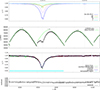 |
Fig. 1. Rectification of a CTIO/CHIRON echelle spectrum (ktc00027) in the region of the Hα line (6563 Å), using the resimplex3 method. Top: Synthetic spectra were computed from our model in Table 1, ‘all-data’ column. Four component spectra (Aa, Ab, B, C) and the resulting spectrum are plotted. Second row: Observed spectrum from CHIRON (black), orders r = 39 to 41, and the corresponding blaze function (green). Third row: Rectified spectrum (black), its comparison to the synthetic spectrum (blue), and corresponding residuals (red). The rectification was done with respect to the continuum level, with interpolation of the blaze parameters over wide lines (cyan) and problematic orders, also avoiding locations of the telluric lines (green). Bottom: Residuals plotted separately. |
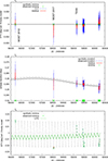 |
Fig. 2. Reference model of ξ Tau, showing ETVs (top), eclipse durations (middle), perturbations with respect to a two-body ephemeris (bottom), MOST and TESS observations (blue), model (grey), residuals (red), and, for reference, observed minima (green). The total χ2 = 1553 (see Table 1 for individual contributions). The mean ephemeris used in the bottom panel is P = 7.146665 d, T0 = 2456224.704705. Our model is certainly able to explain the major perturbations, which are substantial (±0.02 d, or ±30 min), but some systematics remain to be explained (up to 0.002 d, or 3 min). |
3.2. Models constrained by interferometry
Next, we computed a grid of models including three more interferometric data sets (VIS, CLO, T3). Our aim was to constrain the total mass, msum, and the distance, d, and to exclude alternative solutions. We used 121 pairs of msum and d values and fixed these parameters, but all other parameters were set free; each model was re-converged so that it adapts ‘at all cost’.
The results in Fig. 3 show logical correlations between msum, d, as required by astrometric or interferometric data sets (i.e. angular separations of the third and fourth components). However, other data sets (RV, ETV, SED, SED2) are orthogonal to this because some scales are set absolutely, in km s−1, days, and W m−2 m−1, respectively. This implies a uniqueness of the best-fit solution (Table 1). How this solution with χ2 = 1553 looks graphically is shown in Fig. 4. In either case, the ξ Tau distance must be around 66.0 pc; the Gaia distance of 59.6 pc was excluded.
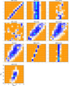 |
Fig. 3. Best-fit models of ξ Tau constrained by multi-technique observations for two fixed parameters, the total mass msum and the distance d. The χ2 values (colours) indicate best fit (cyan), good fits (blue), and poor fits (orange); the overall best fit (red) has χ2 = 1661 (unreduced). We tested 121 pairs of parameters and 3000 sequential iterations of simplex, i.e. 3.6 × 10⁵ models in total. Other dynamical parameters (except msum, d) were free; other radiative parameters were fixed (Nemravová et al. 2016). We constrained the model by SKY, RV, ETV, ECL, SED, SED2 data sets; we did not use interferometry (but we used SKY), spectroscopy (but RV), or light curves (but ETV, ECL). We assumed unit weights, except wetv = wecl = 100, because we wanted to exclude all models with incorrect dynamics. The two parameters are often positively correlated (e.g. SKY, VIS, CLO, T3), as predicted (Kepler 1619), but some data sets are distance independent or orthogonal (RV, ETV, SED, SED2), and the model is considered well constrained. After re-convergence (green), the χ2 further decreased to 1553. The Gaia distance of 59.6 pc was excluded. Additionally, VIS, CLO, and T3 were also computed, but their weights were set to zero, otherwise our model would exhibit tension between VIS and CLO. |
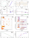 |
Fig. 4. Best-fit model from Fig. 3 with χ2 = 1553 (unreduced). Plots for each data set, SKY, RV, ETV, ECL, VIS, CLO, T3, SED, and SED2, contain observations (blue), synthetic data (yellow), and residuals (red). The best-fit distance is d = 66.0 pc. One can notice some systematics for ETV (see MOST 2017), VIS, or CLO data sets. |
3.2.1. MCMC analysis.
For this model, we estimated the uncertainties of model parameters with the Markov chain Monte Carlo (MCMC) method (Markov 1906), which should reflect the uncertainties of observational data. Here, we used all dynamical parameters, but not all radiative ones, in order to prevent systematics from affecting the resulting uncertainties. If any systematics are present (e.g. tension between VIS and CLO) it will result in very small, unrealistic uncertainties. The standard corner plot is shown in Fig. B.4.
3.3. Models constrained by CHIRON and TESS observations
Next, we included 44 high-resolution spectra (from CHIRON, one per night) and eight high-precision light curves (from MOST and TESS) and computed another grid of models. Our aim was to better constrain the radiative parameters, in particular the effective temperatures T1 and T3. We used 121 pairs of T1 and T3 values and fixed them, but all other parameters were left free.
The results in Fig. 5 show some data sets that are insensitive to the radiative parameters (e.g. SKY, RV, ETV, ECL), but others constrain the temperatures very well (VIS, LC, SYN). In particular, light curves and eclipse depths are very ‘strict’ constraints (T1 ≃ 11000 K, T3 ≃ 14000 K), which is fully in agreement with spectral line profiles. The third component does not eclipse anything, but its brightness contributes as a third light. The line profiles of Aa, Ab, B components are blended, but easy to disentangle because of different rotation speeds (Fig. B.2).
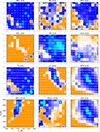 |
Fig. 5. Same as Fig. 3 but for two different fixed parameters, the effective temperatures T1and T3. This time, light curves (LC) and synthetic spectra (SYN) were included. The overall best fit χ2 = 3639180 (unreduced). One can notice some systematics; for example, there is tension between VIS and CLO, the best ECL is offset, the best SED is offset, and the best SED2 is very offset. |
3.3.1. Tension.
Looking at individual contributions to the χ2 versus the position of the best-fit model (Fig. 5, red circle), one can notice the following problems. On one hand, the CLO data set exhibits tension (with respect to VIS), where better fits of CLO data require lower T3. On the other hand, SED, SED2 data sets exhibit different tension (with regard to LC, SYN), requiring higher T3. It is clearly not easy to correct these issues by changing T3, or, as a matter of fact, by changing any other parameter; we note that all other parameters were free.
3.3.2. Systematics.
There might be various reasons for such inconsistencies. First, our model could be internally inconsistent; for example, the light curve algorithm (Wilson & Devinney 1971; Wilson et al. 2010), which is technically comparable to Prša et al. (2016), could be incompatible with grids of synthetic spectra (Lanz & Hubený 2003, 2007; Palacios et al. 2010; de Laverny et al. 2012; Husser et al. 2013) used for fitting of the SYN data set. Second, some approximations might be inadequate; for example, the third component is a fast-rotating star, but we used a synthetic spectrum suitable for slow-rotating stars. The same is true for the interferometric quantities, or VIS, CLO, and T3, where we assumed limb-darkened discs (Hanbury Brown et al. 1974). Third, some fixed parameters might be set incorrectly, for example the linear limb-darkening coefficients, for which we assumed standard values (van Hamme 1993). Fourth, discretisation errors might be larger than expected, especially for the ETV, ECL data sets, where we used a linear interpolation between the neighboring time steps. We checked for all of the possibilities above, but none of them explain the tension.
3.3.3. Best fit.
How the best-fit solution with χ2 = 3639180 looks is shown in Fig. 6. The fit of the SKY data set is acceptable; new WDS data of the fourth component are fitted perfectly, the NPOI data of the third component exhibit only minor systematics. Note that the coordinates are photometric with respect to Aa+Ab or Aa+Ab+B, respectively. The RVs are also acceptable; new CHIRON data are fitted perfectly, in agreement with line profiles (SYN); old RV data exhibit offsets up to 5 km/s, but not systematically. For the ETVs, the offsets are < 0.001 d, but one can notice a trend that MOST 2012 is fitted, TESS is fitted, but MOST 2017 is offset by −0.0015 d. It is clearly not easy to correct these issues, within the current dynamical model (see Sect. 3.4). We verified that the transversal light-time effect (Conroy et al. 2018; Vokrouhlický 2026) has a substantially smaller amplitude. Similar related offsets are seen in the ECL dataset, in agreement with light curves. The fits of VIS, CLO, and T3 data sets contain individual offsets for certain baselines, B/λ, but the trends of V2(B/λ) are correct. This is often caused by visibility calibration, or transfer-function issues. The synthetic SED data set is overestimated (by 0.1 to 0.15 mag), while SED2 is underestimated (by ∼0.3 mag). This might suggest an issue related to the fourth component, the total mass, msum, or the distance, d, but more likely to radiative parameters (see the discussion of T3). The light-curve fit seems to be almost perfect for both the primary and secondary minima, but there are tiny, statistically significant offsets in minima timings, corresponding 1:1 to the ETV offsets above. The fit of normalised spectra (SYN) is also acceptable, including the Hα, Hβ wings, with a notable exception of the Hα, Hβ core depths for Aa, Ab components, which are slightly underestimated. This might suggest an issue related to the grids of synthetic spectra or relative luminosities of the components (Aa, Ab, B).
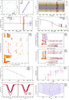 |
Fig. 6. Best-fit model from Fig. 5 with χ2 = 3639180 (unreduced). The light curves (LCs) were phased, to show different minima depths (MOST versus TESS). The synthetic spectra (SYN) plot presents only a subset of ten spectra and only the Hβ line region. One can still notice some systematics for ETV (MOST 2017 offset), ECL (TESS offset), VIS (individual observations), CLO (individual observations), SED (overestimated), SED2 (underestimated), or SYN (Aa, Ab line depths are not sufficient). |
3.4. Models with tides and oblateness
In order to explain the trend seen in ETVs, in particular the negative offset −0.0015 d of the MOST 2017 timings (Fig. 6), we tested models with tides and oblateness2. These terms induce a change of the period (Ṗ) and an additional precession ( ,
,  ), which is added to the existing precession due to four bodies. At the same time, we revised the uncertainties of ETVs to 10−4 d, in agreement with high-precision light curves and our aim to explain offsets at this level. We computed a grid of models parametrised by the oblateness, C20, and the time lag, Δt (Mignard 1979). Only the closest components (Aa, Ab) are relevant, as the remaining (B, C) are too distant and the terms are negligible. For simplicity, we also assumed no misalignment and no spin precession.
The results in Fig. 7 show a clear signal for tides, but not for oblateness. The time lag, Δt, was about (800 ± 100) s when only the first orbit was free. If the second and third orbits were also free, the time lag could be as low as ∼100 s, but only at the expense of a poor fit of the ECL data set (Fig. 8).
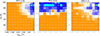 |
Fig. 7. Same as Fig. 3 but for different fixed parameters, i.e., the oblateness, C20, 1, and the tidal time lag, Δt1. For the second component we assumed the same values. The uncertainties of ETVs were revised to 10−4 d. We tested 121 pairs of parameters, 300, 300, and 1000 sequential iterations of simplex: 1.9 × 10⁵ models in total. The parameters of the inner Aa+Ab orbit (plus P2) were free. The best fit is indicated (red) along with a statistically equivalent, close-to-zero C20, 1 solution (green). Zero Δt1 is excluded. |
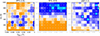 |
Fig. 8. Same as Fig. 7 but the parameters of all orbits were free. The solutions differ from Fig. 7 partly because of perturbations by component C. The solutions with low Δt1 ∼ 100 s exhibit a poor fit of eclipse duration (ECL), so the solution with high Δt1 (and zero C20, 1) is still preferred. |
We computed the tides for the reference radius R = R⊙, the Love number k2 = 0.3, the mean motion n ≐ 0.879 rad d−1, and the rotation frequency ω = 1.25 rad d−1. One can rescale Δt to any radius, for example R′=R1 (and k2′ = 0.03), because the tidal term is proportional to R5k2Δt, so
 (6)
(6)
One can convert it to the dissipation factor
 (7)
(7)
or equivalently to Q′≡Q/k2 ≃ 5500, or to  .
.
This seems to be too high for non-rotating B-type stars (Δt ≃ 0.15 s, Q ≃ 106, Q′≃3 × 10⁷, E ≃ 2 × 10⁻⁸; Zahn 1975, 1977).
With this point of view in mind, the model with tides was excluded. We point out just a few arguments as to why dissipation could be larger than expected. Some stars orbited by exoplanets have substantially smaller Q′≃5 × 10⁴ (Penev et al. 2018; Maciejewski et al. 2016). Rotating stars exhibit Eddington–Sweet circulation (Eddington 1925; Sweet 1950), Soldberg–Høiland instability (Solberg 1936; Høiland 1941), or Goldreich–Schubert–Fricke instability (Goldreich & Schubert 1967; Fricke 1968), and such stars have smaller Q′. Some binaries show signs of large-amplitude, resonant oscillation, not only at the orbital frequency (‘heartbeat’), but at much higher multiples, for example 229 times (Fuller et al. 2017; Fuller & Felce 2024). Finally, the inner orbit (Aa+Ab) has non-zero, forced eccentricity, e → 0.008, due to component B, which increases dissipation as on Io (e = 0.004; Peale et al. 1979).
Alternative solutions also exist for non-zero oblateness, for example C20, 1 = C20, 2 = −0.001. Whether or not it is reasonable can be estimated from rotational and tidal (Roche) deformation. Assuming a Love number (Love 1909) of the order of k2 ≃ 0.01 to 0.1 for radiative and convective stars, respectively (Claret 2004), the oblateness from rotation is (Kaula 1966)
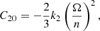 (8)
(8)
and from tides
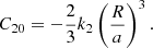 (9)
(9)
The maximal value (convective, rotational) is ∼1.5 × 10⁻⁴. This is why the model with oblateness was also excluded.
3.5. Models with five components ((Aa+Ab)+B)+(Ca+Cb))
Since some tension remains in the current model – specifically (i) high-precision astrometry (Tokovinin et al. 2020), leads to slightly more ‘elongated’ outer orbit; (ii) the RV dataset constrains the masses of components Aa, Ab, B; (iii) the ETV data set would require more massive component C; (iv) the SED dataset larger distance (69 pc); and (v) the SED2 data set a fainter component C – an elegant solution would be splitting of component C into a binary (Ca+Cb). This decreases its luminosity by up to ∼2.25 mag, depending on the mass ratio.
We computed the same grid of models as in Sect. 3.4. The results in Fig. 9 show a few solutions with non-zero tides, Δt = (100 ± 50) s, which is a more reasonable value than in Sect. 3.4, because it corresponds to Δt′ = 90 s, Q = 1300, Q′ = 44000, E = 1.5 × 10⁻⁵. Most importantly, though, this solution is no longer in contradiction with the ECL dataset, or the dynamics of the inner eclipsing binary. This confirms that a five-component model is necessary to correctly describe the ξ Tau system.
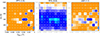 |
Fig. 9. Same as Fig. 7 but for models with five components (Aa+Ab+B+Ca+Cb). The perturbations and the light-time effect due to Ca+Cb components were stronger. The best-fit solution with low Δt1 ∼ 100 s now exhibits a good fit of eclipse duration (ECL). |
4. Temporal evolution of ξ Tau
4.1. Signs of secular evolution
The ξ Tau system is appreciably compact to reveal temporal evolution of its individual orbits. In particular, the observations available to date require the orbital elements of the eclipsing pair (Aa+Ab) and of the third component (B) to evolve according to our dynamical model (Fig. 12). These variations occur over various timescales: (i) the shortest (days to a year) is defined by the orbital periods P1 and P2; (ii) the intermediate (decades to centuries) by the orbital period, P3, or the precession rates  ,
,  ,
,  , expressed in the Laplace reference frame, whose z-axis coincides with the angular momentum of the (Aa+Ab)+B triple; and (iii) the longest (millenia to 105 years) is given by the slow precession rate
  .
.
4.1.1. Shortest timescales.
The mutual gravitational interaction in the (Aa+Ab)+B triple makes the shortest timescale apparent in the periods P1 and P2 (or equivalently, the semi-major axes a1 and a2) as well as the eccentricities e1 and e2. We find that e1(t) oscillates between 0 and 0.008, which is dominated by short-period terms with P1 and P2 periods and amplitudes ≃0.003 and ≃0.004. These variations of e1 are necessary to explain the exact eclipse timings, namely the contribution that cannot be produced by the perturbation of the binary’s mean motion by star B.
4.1.2. Intermediate timescales.
The correlated variations of inclinations i1 and i2, as well as the nodal longitudes Ω1 and Ω2 in the observer’s reference frame, occur with the periodicity of PΩ ≃ 7000 d. The projected inclination, i1, of the inner eclipsing binary changes from 86.1° to 87.1°, an effect clearly manifested in eclipse durations and depths, according to the precise photometric measurements by MOST (2012 and 2017) and TESS (from 2020 to 2023). These variations appear to be a consequence of a simple precession of the orbital angular momenta LA and LB of the Aa+Ab binary and of the component B orbit about their composite angular momentum, LAB = LA + LB. In particular, both LA and LB describe coni with small opening angles of about LAB with the period PΩ, keeping their mutual angle J1 nearly constant. Due to the very small value of e1, the argument of periastron, ω1, is an ill-defined orbital element (especially near epochs when e1 ≃ 0), and its fast circulation is not a representative secular effect. In contrast, the argument of periastron, ω2, of orbit B exhibits in the observer’s reference frame a regular precession with a rate of 2.1° y−1 (see Nemravová et al. 2016 and Fig. 12). This effect is evidenced by the measured RVs of components Aa, Ab, and B.
In order to explore the behaviour of the orbital eccentricity, e1, of the eclipsing binary Aa+Ab on intermediate timescales, we digitally filtered the signal with periods P1 and P2 from the time series of osculating values of e1. The secular theory of triple dynamics (e.g. Georgakarakos 2003, 2009; Breiter & Vokrouhlický 2015) predicts two contributions to e1, namely (i) the free (proper) component, depending on the initial conditions, and (ii) the forced component, due to the presence of the third star (B) and its perturbations. We found that the forced component with an amplitude of 7.6 × 10⁻⁴ and a period of 167 yr (i.e. the apsidal precession timescale of ω2) dominates the evolution of e1, leaving no signal corresponding to the free component. This result suggests that the free component of e1 has been damped by the past tidal evolution in the binary Aa+Ab, a process that is currently witnessed by the weak tidal signal (Sect. 3.4).
4.1.3. Longest timescales.
The variations over the longest timescales are associated with the outer orbit of component C (P3 ≐ 18900 d ≐ 52 y). The gravitational perturbation of orbit B during the orbital motion of C is clearly manifested in the measured RVs. It is amplified near the periastron passage of C in July 2008 due to its large eccentricity, e3 ≃ 0.573. An interesting ‘sawtooth’ structure seen during the sudden increase of i2 between JD 2454000 and 2455000 (an interval of time extending approximately 1.5 y before and after the periastron passage of C; Fig. 12) may be explained as a coherent effect during five or six conjunctions between components B and C, repeating themselves after 145 d. We verified that the conjunctions occur at the same geometrical configuration, implying that the out-of-plane perturbing acceleration, W, in orbit B maintains the same sign. Consequently, since di/dt ∝ Wcos(f + ω) (Gauss 1809), the perturbing effect on i2 accumulates coherently.
4.2. Stability
The gravitational perturbations also operate on timescales longer than centuries, beyond what is evidenced by the available observations. We thus conducted numerical integrations over 105 y to study the stability of the ξ Tau system. We assumed the four-component model from Sect. 3.2. The integrator was the same, the Bulirsch–Stoer with an adaptive time step, but we used a smaller tolerance, ϵ = 10−10, to assure the angular momentum conservation.
We found that the ((Aa+Ab)+B)+C hierarchy is stable, with all components moving in a well-orchestrated manner. Apart from the (Aa+Ab)+B inner triple, where LA and LB precess about LAB, as discussed in Sect. 4.1, we note that the nodal period PΩ is smaller than P3 (and non-resonant). This implies that the corresponding nodal period at the higher level in the ξ Tau hierarchy, namely the precession of LAB and LC about Lsum is much longer, i.e. ≃85000 y according to our model.
4.2.1. Non-existent Kozai oscillations.
For comparison, we tested a three-body model of ξ Tau, where the Aa+Ab binary was replaced with a single component A. This totally changed the overall orbital evolution, because of the Kozai oscillations (von Zeipel 1910; Lidov 1961; Kozai 1962). As illustrated in Fig. 11, the eccentricities e2, e3 and inclinations i2, i3 exhibit coupled oscillations, with a period of ≃11500 y. The peak value of e2(t) is 0.8, which would destabilize the innermost binary Aa+Ab. Nevertheless, the stability of the (Aa+Ab)+B sub-system is ensured by a protection mechanism, consisting of its own mutual interaction, which induces the periastron precession,  , with a period of only 180 y. This is much shorter than the Kozai timescale, effectively switching off the Kozai mechanism.
An interesting implication of the fact that LC ≫ LAB (see Fig. 10) is that the opening angle of the cone described by LAB is relatively large (47°). As a result, the viewing geometry of the eclipsing binary (Aa+Ab) changes significantly over millennia. We predict eclipses will vanish in 18000 y from now.
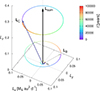 |
Fig. 10. Angular-momentum vectors of the ξ Tau sub-systems (Aa+Ab, B, C) and their long-term evolution. The coordinates were rotated to the Laplace reference frame, with the z-axis along the total angular momentum, Lsum, of the whole ξ Tau system (in absence of external torques Lsum is constant). The individual contributions were obtained as |

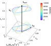 |
Fig. 11. Same as Fig. 10 but only for three bodies (A, B, C), where A represents Aa+Ab. Without a protection mechanism, the Kozai oscillations were triggered, with a period of ≃11500 y. The angular momenta LB and LC still describe conical surfaces, but now their mutual angle J exhibits large oscillations, which triggers correlated oscillation of eccentricities and inclinations of the inner and outer orbits. |
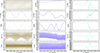 |
Fig. 12. Osculating orbital elements of ξ Tau in the course of time, for the model with χ2 = 3639180. The angular elements are expressed in the observer’s reference frame. See the description in the main text. |
5. Discussion
5.1. Photocentre motion in Gaia DR4
In order to understand how the multiplicity of ξ Tau influences its parallax measurements (Vallenari et al. 2023), we computed its photocentre motion. The simplest, five-parameter model suitable for single stars consists of the position α, δ, the proper motion (PM) μα, μδ, and the parallax π. We added to this model the photocentre, computed as an average of barycentric positions, weighted by the passband fluxes of components Aa, Ab, B, and C. For reference, the Gaia G filter has λeff = 639.02 nm, Δeff = 317.32 nm and the respective weights were 0.181, 0.173, 0.603, and 0.042. Our results (Fig. 13) show that the overall photocentre motion within the observational time span of Gaia reaches almost 40 mas. However, this can be compensated by using different PM values, specifically μα′ = 67.0 mas y−1, μδ′= − 40.5 mas y−1. In other words, the new trajectory on the sky was adjusted so that its end points correspond to the old trajectory.
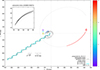 |
Fig. 13. Photocentre motion of the ξ Tau system and its influence on parallax measuments. We plot the orbital motion of individual components Aa, Ab, B, C in the barycentric frame (light gray or coloured, if within the observational timespan of Gaia), the photocentre motion (black), the parallactic motion (gray), the proper motion (light gray), and all contributions with the new parallax π′ = 14.717 mas (cyan). For comparison, we plot all contributions with the old parallax π = 16.791 mas (light cyan) and also the old trajectory from Gaia DR3 (dash-dotted). |
Now the photocentre motion consists of two contributions: (i) 6 mas oscillating due to the triple (Aa+Ab)+B; and (ii) 4 mas curved due to component C. These offsets were most likely responsible for an incorrect value of π = 16.791 mas in Gaia DR3. When we used our preferred distance (67.9 pc), corresponding to π′ = 14.717 mas, the new trajectory became closer to the old trajectory, or the actual measurements. Consequently, our model explains not only all kinds of observations, but also why the Gaia DR3 parallax is offset. We do expect that binary, triple or quadruple astrometric models in Gaia DR4 will confirm our results.
5.2. Oscillations
In order to better understand rapid low-amplitude variability of ξ Tau (Nemravová et al. 2016), we used the new photometric data from TESS to compute a new periodogram. After excluding all eclipse intervals to suppress the orbital frequency, forb (and its harmonics), we actually computed a sequence of periodograms (Lenz & Breger 2005), revealing two dominant frequencies, f1 = 1.407 d−1, f2 = 2.371 d−1, with amplitudes of approximately 7 and 5 × 10⁻⁴ in the relative flux (Fig. 14). The corresponding periods are 0.710 and 0.421 d, respectively. The overall time span (1115 d) allowed us to reach the resolution of 1/Δ = 10−4 d−1.
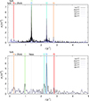 |
Fig. 14. Periodogram of ξ Tau from the TESS (top) and MOST 2012 (bottom) light curves. We removed eclipses and computed five Fourier transforms (Lenz & Breger 2005), with fitting of frequencies, amplitudes and phases, and subtracting the respective model, ∑iAisin[2π(fit + ϕi)]. For TESS, the dominant frequencies were 1.407, 2.371, 1.421, 2.814, and 0.279 d−1. We note f4 = 2f1 and f5 = 2forb of the inner orbit. For MOST 2012, on the contrary, we found 2.369, 2.216, 0.993, 0.282, and 2.839 d−1. The non-existent 1.407 d−1 frequency is labeled “ftess”. |
The f2 frequency is persistent and could be attributed to rotation of the third component (Nemravová et al. 2016). Its rotational broadening of vrot3 = 242 km s−1 corresponds to the upper limit of Prot3 ≤ 0.472 d. The rotational axis inclination is unknown, but in order to obtain 0.421 d, it should be ∼60°.
The f1 frequency should also be attributed to the third component, which is most likely a slowly pulsating B star (SPB; Waelkens & Rufener 1985). The star is located in the instability strip of g-modes of the order of ℓ = 1 or 2 (Sharma et al. 2022). However, there is a problem with non-existent f1 oscillations in the MOST 2012 data, and no evidence of damping in the TESS 2020–2023 data. A possible explanation may consist of interference (‘beat’) of two nearby frequencies (e.g. Sharma et al. 2022, Fig. 5). However, the time resolution of the TESS photometry is insufficient to identify frequencies (f1, f1′) whose combination would result in conjectured beats (f1 − f1′) separated by more than eight years.
We verified that the reason for missing f1 oscillations is not technical. The MOST telescope is a Maksutov–Cassegrain with a Fabry lens placed in the secondary focus (Walker et al. 2003). Its diaphragm (0.117 mm) corresponds to the angular diameter of ϕ = d/f = 27″, which is too large to miss light from the fourth component (up to 600 mas).
Still on a technical note, the TESS satellite observed ξ Tau as an over-exposed target, with blooming (Ricker et al. 2015; Krishnamurthy et al. 2019). In order to compute a sum of all pixels (both over- and under-exposed) the photometric aperture must be 13 pixels in the y-direction. Since the pixel size is 15 μm and the focal length is 146 mm, the angular distance is up to ϕ = 4.2′. Using Lightkurve (Cardoso et al. 2018), we checked stars in the surroundings. In particular, TIC 399947175 is close to the aperture, but it does not exhibit such oscillations. So, unfortunately, the f1 oscillations remain an open problem.
6. Conclusions
In this work, we studied the ξ Tau quadruple system using dynamical models of differing complexities, constrained by 11 different types of observations. Using N-body and post-Newtonian terms and assuming four components (Aa, Ab, B, C), we found a global minimum of χ2, where the total mass is 9.55 M⊙ and the distance 66.1 pc (see Table 1). However, such a model still exhibits some tension; for example, minima timings for the MOST 2017 dataset are offset by ∼0.0015 d, the SED is overestimated by 30%, and so on.
It was surprisingly difficult to find a better solution. Eventually, we were forced to use N-body, post-Newtonian, oblateness, and tide terms and assume five components (Aa, Ab, B, Ca, Cb). We found a global minimum–where the total mass is 10.37 M⊙–mainly due to the binary nature of component C and the distance 67.9 pc. Given the increased number of model parameters (36 vs. 44), it is not surprising that the model fits observations better. Nevertheless, the sole behavior of the model, how the minima timings were corrected, how the SED was corrected, suggests that the five-component model is the correct one.
Finally, let us point out that ξ Tau is indeed an interacting stellar system; even the most distant component C, interacts with component B at periastron passage, inducing a non-negligible phase shift, which propagates to the innermost eclipsing binary Aa+Ab, measurably shifting its eclipse timings. This has a potential to detect additional, dwarf, or exoplanetary components with low masses.
Acknowledgments
This work has been supported by the Czech Science Foundation through the grant 25-16507S (M. Brož and D. Vokrouhlický). We thank an anonymous referee for constructive comments. This work is co-funded by the European Union (ERC, MAGNIFY, Project 101126182). Views and opinions expressed are however those of the authors only and do not necessarily reflect those of the European Union or the European Research Council. Neither the European Union nor the granting authority can be held responsible for them. This work has made use of data from the European Space Agency (ESA) mission Gaia, processed by the Gaia Data Processing and Analysis Consortium (DPAC). This research has made use of the SIMBAD database operated at CDS, Strasbourg (France), and NASA’s Astrophysics Data System (ADS). This paper includes data collected by the TESS mission, which are publicly available from the Mikulski Archive for Space Telescopes (MAST). Funding for the TESS mission is provided by NASA’s Science Mission directorate.
References
- Bailer-Jones, C. A. L., Rybizki, J., Fouesneau, M., Demleitner, M., & Andrae, R. 2021, AJ, 161, 147 [Google Scholar]
- Barker, P. K. 1984, AJ, 89, 899 [NASA ADS] [CrossRef] [Google Scholar]
- Borkovits, T. 2022, Galaxies, 10, 9 [NASA ADS] [CrossRef] [Google Scholar]
- Borkovits, T., Rappaport, S. A., Tan, T. G., et al. 2020, MNRAS, 496, 4624 [NASA ADS] [CrossRef] [Google Scholar]
- Božić, H., Harmanec, P., Brož, M., et al. 2026, A&A, in press, https://doi.org/10.1051/0004-6361/202453206 [Google Scholar]
- Breiter, S., & Vokrouhlický, D. 2015, MNRAS, 449, 1691 [NASA ADS] [CrossRef] [Google Scholar]
- Brož, M. 2017, ApJS, 230, 19 [Google Scholar]
- Brož, M., Marchis, F., Jorda, L., et al. 2021, A&A, 653, A56 [Google Scholar]
- Brož, M., Harmanec, P., Zasche, P., et al. 2022a, A&A, 666, A24 [NASA ADS] [CrossRef] [EDP Sciences] [Google Scholar]
- Brož, M., Ďurech, J., Carry, B., et al. 2022b, A&A, 657, A76 [NASA ADS] [CrossRef] [EDP Sciences] [Google Scholar]
- Brož, M., Ďurech, J., Ferrais, M., et al. 2023, A&A, 676, A60 [NASA ADS] [CrossRef] [EDP Sciences] [Google Scholar]
- Brož, M., Conroy, K. E., & Prša, A. 2025, ArXiv e-prints [arXiv:2506.20866] [Google Scholar]
- Bulirsch, R., & Stoer, J. 1966, Numerische Mathematik, 8, 1 [Google Scholar]
- Cardoso, J. V. D. M., Hedges, C., Gully-Santiago, M., et al. 2018, Astrophysics Source Code Library [record ascl:1812.013] [Google Scholar]
- Claret, A. 2004, A&A, 424, 919 [NASA ADS] [CrossRef] [EDP Sciences] [Google Scholar]
- Conroy, K. E., Prša, A., Horvat, M., & Stassun, K. G. 2018, ApJ, 854, 163 [Google Scholar]
- de Laverny, P., Recio-Blanco, A., Worley, C. C., & Plez, B. 2012, A&A, 544, A126 [NASA ADS] [CrossRef] [EDP Sciences] [Google Scholar]
- Eddington, A. S. 1925, The Observatory, 48, 73 [NASA ADS] [Google Scholar]
- Ferrais, M., Jorda, L., Vernazza, P., et al. 2022, A&A, 662, A71 [NASA ADS] [CrossRef] [EDP Sciences] [Google Scholar]
- Fricke, K. 1968, ZAp, 68, 317 [Google Scholar]
- Fuksa, M., Brož, M., Hanuš, J., et al. 2023, A&A, 677, A189 [NASA ADS] [CrossRef] [EDP Sciences] [Google Scholar]
- Fuller, J., & Felce, C. 2024, MNRAS, 527, L103 [Google Scholar]
- Fuller, J., Hambleton, K., Shporer, A., Isaacson, H., & Thompson, S. 2017, MNRAS, 472, L25 [Google Scholar]
- Gallenne, A., Mérand, A., Kervella, P., et al. 2023, A&A, 672, A119 [NASA ADS] [CrossRef] [EDP Sciences] [Google Scholar]
- Gauss, K. F. 1809, Theoria motvs corporvm coelestivm in sectionibvs conicis solem ambientivm [Google Scholar]
- Georgakarakos, N. 2003, MNRAS, 345, 340 [Google Scholar]
- Georgakarakos, N. 2009, MNRAS, 392, 1253 [Google Scholar]
- Goldreich, P., & Schubert, G. 1967, ApJ, 150, 571 [Google Scholar]
- Hanbury Brown, R., Davis, J., Lake, R. J. W., & Thompson, R. J. 1974, MNRAS, 167, 475 [NASA ADS] [CrossRef] [Google Scholar]
- Harmanec, P. 1988, Bull. Astron. Inst. Czech., 39, 329 [NASA ADS] [Google Scholar]
- Harmanec, P. 1998, A&A, 335, 173 [NASA ADS] [Google Scholar]
- Harmanec, P., Horn, J., & Juza, K. 1994, A&AS, 104, 121 [NASA ADS] [Google Scholar]
- Harmanec, P., Lipták, J., Koubský, P., et al. 2020, A&A, 639, A32 [EDP Sciences] [Google Scholar]
- Høiland, E. 1941, Avhandl. utg. av Det Norske Videnskaps-Akademi i Oslo. I. Mat.-Naturv. Klasse, 11 [Google Scholar]
- Holman, M. J., & Wiegert, P. A. 1999, AJ, 117, 621 [Google Scholar]
- Husser, T.-O., Wende-von Berg, S., Dreizler, S., et al. 2013, A&A, 553, A6 [NASA ADS] [CrossRef] [EDP Sciences] [Google Scholar]
- Hut, P. 1981, A&A, 99, 126 [NASA ADS] [Google Scholar]
- Johnson, H. L., Iriarte, B., Mitchell, R. I., & Wisniewski, W. Z. 1966, Commun. Lunar Planet. Lab., 4, 99 [NASA ADS] [Google Scholar]
- Jones, A., Noll, S., Kausch, W., Szyszka, C., & Kimeswenger, S. 2013, A&A, 560, A91 [NASA ADS] [CrossRef] [EDP Sciences] [Google Scholar]
- Kaula, W. M. 1966, Theory of Satellite Geodesy. Applications of Satellites to Geodesy (Waltham, Massachussetts: Blaisdell Publishing Company) [Google Scholar]
- Kepler, J. 1619, Ioannis Keppleri harmonices mundi libri V [Google Scholar]
- Kozai, Y. 1962, AJ, 67, 591 [Google Scholar]
- Krishnamurthy, A., Villasenor, J., Seager, S., Ricker, G., & Vanderspek, R. 2019, Acta Astronautica, 160, 46 [Google Scholar]
- Lanz, T., & Hubený, I. 2003, ApJS, 146, 417 [NASA ADS] [CrossRef] [Google Scholar]
- Lanz, T., & Hubený, I. 2007, ApJS, 169, 83 [CrossRef] [Google Scholar]
- Lenz, P., & Breger, M. 2005, Commun. Asteroseismol., 146, 53 [Google Scholar]
- Levison, H. F., & Duncan, M. J. 1994, Icarus, 108, 18 [NASA ADS] [CrossRef] [Google Scholar]
- Lidov, M. L. 1961, Iskusstvennye Sputniki Zemli, 8, 5 [Google Scholar]
- Love, A. E. H. 1909, Proc. Roy. Soc. Lond. Ser. A, 82, 73 [Google Scholar]
- Maciejewski, G., Dimitrov, D., Fernández, M., et al. 2016, A&A, 588, L6 [NASA ADS] [CrossRef] [EDP Sciences] [Google Scholar]
- Marchis, F., Jorda, L., Vernazza, P., et al. 2021, A&A, 653, A57 [NASA ADS] [CrossRef] [EDP Sciences] [Google Scholar]
- Markov, A. A. 1906, Izvestiya Fiziko-matematicheskogo obschestva pri Kazanskom universitete, 15, 135 [Google Scholar]
- Mason, B. D., Wycoff, G. L., Hartkopf, W. I., Douglass, G. G., & Worley, C. E. 2001, AJ, 122, 3466 [Google Scholar]
- Mignard, F. 1979, Moon Planets, 20, 301 [Google Scholar]
- Nelder, J. A., & Mead, R. 1965, Comput. J., 7, 308 [Google Scholar]
- Nemravová, J. A., Harmanec, P., Brož, M., et al. 2016, A&A, 594, A55 [Google Scholar]
- Noll, S., Kausch, W., Barden, M., et al. 2012, A&A, 543, A92 [NASA ADS] [CrossRef] [EDP Sciences] [Google Scholar]
- Oplištilová, A., Mayer, P., Harmanec, P., et al. 2023, A&A, 672, A31 [NASA ADS] [CrossRef] [EDP Sciences] [Google Scholar]
- Palacios, A., Gebran, M., Josselin, E., et al. 2010, A&A, 516, A13 [NASA ADS] [CrossRef] [EDP Sciences] [Google Scholar]
- Peale, S. J., Cassen, P., & Reynolds, R. T. 1979, Science, 203, 892 [Google Scholar]
- Penev, K., Bouma, L. G., Winn, J. N., & Hartman, J. D. 2018, AJ, 155, 165 [NASA ADS] [CrossRef] [Google Scholar]
- Perryman, M. A. C., & ESA 1997, The HIPPARCOS and TYCHO Catalogues (Noordwijk, Netherlands: ESA Publications Division) [Google Scholar]
- Pietrzyński, G., Graczyk, D., Gieren, W., et al. 2013, Nature, 495, 76 [Google Scholar]
- Pietrzyński, G., Graczyk, D., Gallenne, A., et al. 2019, Nature, 567, 200 [Google Scholar]
- Piskunov, N., Wehrhahn, A., & Marquart, T. 2021, A&A, 646, A32 [NASA ADS] [CrossRef] [EDP Sciences] [Google Scholar]
- Prša, A., Conroy, K. E., Horvat, M., et al. 2016, ApJS, 227, 29 [Google Scholar]
- Ricker, G. R., Winn, J. N., Vanderspek, R., Latham, D. W., & Bakos, G. 2015, J. Astron. Telesc. Instrum. Syst., 1, 014003 [Google Scholar]
- Rowan, N. 1990, Ph.D. Thesis, Univ. Texas Austin [Google Scholar]
- Sharma, A. N., Bedding, T. R., Saio, H., & White, T. R. 2022, MNRAS, 515, 828 [NASA ADS] [CrossRef] [Google Scholar]
- Škoda, P., Šurlan, B., & Tomić, S. 2008, SPIE Conf. Ser., 7014, 70145X [Google Scholar]
- Solberg, H. 1936, Astrophysica Norvegica, 1, 237 [Google Scholar]
- Standish, E. M., & Williams, J. G. 2006, Orbital Ephemerides of the Sun, Moon, and Planets (University Science Books) [Google Scholar]
- Sweet, P. A. 1950, MNRAS, 110, 548 [Google Scholar]
- Thebault, P., & Bonanni, D. 2025, A&A, 700, A106 [NASA ADS] [CrossRef] [EDP Sciences] [Google Scholar]
- Thebault, P., & Haghighipour, N. 2015, in Planetary Exploration and Science: Recent Results and Advances, eds. S. Jin, N. Haghighipour, & W. H. Ip, 309 [Google Scholar]
- Tokovinin, A. 2021, Universe, 7, 352 [NASA ADS] [CrossRef] [Google Scholar]
- Tokovinin, A., & Moe, M. 2020, MNRAS, 491, 5158 [NASA ADS] [CrossRef] [Google Scholar]
- Tokovinin, A., Fischer, D. A., Bonati, M., et al. 2013, PASP, 125, 1336 [NASA ADS] [CrossRef] [Google Scholar]
- Tokovinin, A., Mason, B. D., Mendez, R. A., Costa, E., & Horch, E. P. 2020, AJ, 160, 7 [NASA ADS] [CrossRef] [Google Scholar]
- Vallenari, A., Brown, A. G. A., Prusti, T., et al. 2023, A&A, 674, A1 [NASA ADS] [CrossRef] [EDP Sciences] [Google Scholar]
- van Hamme, W. 1993, AJ, 106, 2096 [Google Scholar]
- Vokrouhlický, D. 2026, A&A, 709, A63 [NASA ADS] [CrossRef] [EDP Sciences] [Google Scholar]
- von Zeipel, H. 1910, Astron. Nachr., 183, 345 [Google Scholar]
- Waelkens, C., & Rufener, F. 1985, A&A, 152, 6 [NASA ADS] [Google Scholar]
- Walker, G., Matthews, J., Kuschnig, R., et al. 2003, PASP, 115, 1023 [Google Scholar]
- Wilson, R. E., & Devinney, E. J. 1971, ApJ, 166, 605 [Google Scholar]
- Wilson, R. E., Van Hamme, W., & Terrell, D. 2010, ApJ, 723, 1469 [NASA ADS] [CrossRef] [Google Scholar]
- Xu, X., Cisewski-Kehe, J., Davis, A. B., Fischer, D. A., & Brewer, J. M. 2019, AJ, 157, 243 [NASA ADS] [CrossRef] [Google Scholar]
- Zahn, J. P. 1975, A&A, 41, 329 [NASA ADS] [Google Scholar]
- Zahn, J. P. 1977, A&A, 57, 383 [Google Scholar]
In the context of stellar studies, these effects are commonly denoted equilibrium and non-equilibrium tides (e.g. Hut 1981).
Appendix A: Rectification of CTIO/CHIRON spectra
As a prerequisite, one has to describe the CTIO/CHIRON instrument, in order to rectify all observed spectra and minimize systematics, in particular, in the Balmer lines wings. This required redefinition of the blaze function. The rectification is defined as
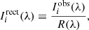 (A.1)
(A.1)
where Iirect(λ) is the rectified spectrum, Iiobs(λ) the observed spectrum, R(λ) the rectification function; in the case of an echelle spectrum, it is called the ‘blaze function’. The motivation for rectification is to avoid absolute calibration, to measure line profiles, and to compare to normalized synthetic spectra. For complex echelle spectra, a number of methods exist: spline fitting, using a reference spectrum, a theoretical blaze function, α-shapes (Xu et al. 2019), or optimal extraction (Piskunov et al. 2021).
In the case of spline fitting (e.g. Harmanec et al. 2020), parts considered as continuum are fitted with a cubic spline, where the spline extends over wide lines. Among the common problems is uncertain continuum level, uncertain line wings, or unreliable log g values. Moreover, in the Paschen series region, overlapping lines and missing continuum make reliable rectification impossible.
In the case of a reference spectrum (Škoda et al. 2008), a rectified spectrum of a similar star is used. Alternatively, it could be a spectrum rectified by splines, obtained by comparison to a suitable synthetic spectrum. A measured spectrum is then divided by a reference spectrum (Eq. (A.1)), to get R(λ). Of course, this cannot be done without a low-noise reference spectrum. Among the common problems is noise in the reference spectrum, mismatch of resolution, or rapid changes.
Rectification by a theoretical blaze function (Barker 1984) assumes that
![Mathematical equation: $$ \begin{aligned} R(\lambda ) = A_r \left\{ {\sin \left[\pi \alpha _r X_r(\lambda )\right] \over \pi \alpha _r X_r(\lambda )}\right\} ^2\quad \mathrm{for}\; \forall r, \end{aligned} $$](/articles/aa/full_html/2026/07/aa60047-26/aa60047-26-eq22.gif) (A.2)
(A.2)
where the coefficients are different for each order r, and
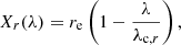 (A.3)
(A.3)
where λ is the wavelength, λc the central wavelength, A the local maximum of the blaze function, re the echelle order; we use our own numbering of orders
 (A.4)
(A.4)
The grating constant
 (A.5)
(A.5)
where l is the width of a grating facet, 1/d the spatial frequency of facets, γ the blaze angle.
Unfortunately, Eq. (A.2) only accounts for the basic grating theory. Slight variations are not included and it does not represent the actual CTIO/CHIRON data. The blaze function thus needs more degrees of freedom and our method is based on this approach.
A.1. Redefined blaze function
We proposed the following redefinition of the blaze function
![Mathematical equation: $$ \begin{aligned} R(\lambda ) = A_r \left\{ {\sin \left[\pi \beta _r(\lambda )X_r(\lambda )\right]\over \pi \beta _r(\lambda )X_r(\lambda )}\right\} ^2 \quad \mathrm{for}\; r = 1..62, \end{aligned} $$](/articles/aa/full_html/2026/07/aa60047-26/aa60047-26-eq26.gif) (A.6)
(A.6)
where the constant αr is replaced with the function
 (A.7)
(A.7)
while Xr(λ) remained the same as in Eq. (A.3); λc, r, Ar, αr, δr, γr, θr, εr are order-dependent parameters, which we determined by fitting.
We defined the respective metric as
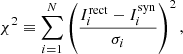 (A.8)
(A.8)
where Iirect is the rectified observed intensity, Iisyn is the intensity of the synthetic (rectified) spectrum; the uncertainties
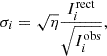 (A.9)
(A.9)
where Iiobs is the observed (not rectified) intensity, η is the gain of the CCD detector.
Synthetic spectra were taken from our previous, converged model of ξ Tau (Nemravová et al. 2016). They served primarily to estimate the continuum level, not the depths of lines. We avoided the telluric lines, as obtained by the Skycalc tool (Noll et al. 2012; Jones et al. 2013) for the nearest available observatory, which is La Silla. The positions of the respective lines were masked in observed spectra.
In total, one has 2 parameters per-order and per-dataset (λc, r, Ar) and 5 parameters per-order (αr, δr, γr, θr, εr), the number of orders is 62, the number of datasets is 10 (since we selected a subset, evenly distributed in time), which implied 1550 parameters. We optimized their values by the simplex algorithm (Nelder & Mead 1965), order by order. We call this first, direct method ‘resimplex1’. 3 The resulting blaze function is shown in Fig. A.1, and it is significantly better than our own, manual rectification.
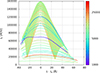 |
Fig. A.1. Redefined blaze function R(λ), according to (Eq. (A.6)), estimated for CTIO/CHIRON spectra. It is plotted in absolute, analog-digital units (adu) and for shifted wavelengths λ − λc, r, for each order r. The rectification method was resimplex1. Colours correspond to χ2 contributions. The total χ2 = 666239 (unreduced) is a measure of correspondence between the rectified observed spectra and the synthetic (rectified) spectra. |
A.2. Constrained blaze function
Alternatively, in order to decrease the variability of the blaze function, some parameters were approximated by polynomials
 (A.10)
 (A.11)
 (A.12)
 (A.13)
 (A.14)
while R(λ) and βr(λ) functions remained the same. In the 1st step, the respective coefficients were estimated by fitting these polynomials to αr, γr, δr, θr, εr discrete values (Fig. B.1). The remaining parameters λc, r, Ar were taken from Appendix A.1. In the 2nd step, we further optimized a1, a2, …, e4, e5, and λc, r, Ar were periodically updated during convergence, in order to improve their consistency with the polynomials. We again worked with 62 orders, 10 datasets, which implied 1265 parameters. We call this second, constrained method ‘resimplex2’.
In order to avoid problems with wide lines, we did not use the following orders for fitting (in Å): #7 4732.3–4786.8 Hβ, #8 4772.3–4827.3 Hβ, #9 4813.1–4868.5 Hβ, #10 4854.5–4910.5 Hβ, #11 4896.7–4953.2 Hβ, #39 6472.5–6547.0 Hα, #40 6547.7–6623.1 Hα, #44 6867.1–6946.1 telluric lines, #52 7609.5–7697.0 telluric lines, #57 8160.9–8254.7 telluric lines. The polynomials (Eqs. (A.10)–(A.14)) then serve as interpolants for these regions.
The result is shown in Fig. A.2. The χ2 is higher, but still better than our manual rectification. The biggest contribution is from the last four orders (i.e. the Paschen series).
A.3. Constrained central wavelengths
In order to further decrease the order-to-order variability, we constrained the central wavelength as
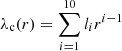 (A.15)
and also the amplitude as
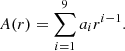 (A.16)
This turned out to be the compromise between simplicity and complexity, keeping low χ2. However, both λc(r) and Ar(r) must be different for each dataset, because they are directly related to the variability of the atmosphere (extinction, refraction). Other blaze parameters were taken from Appendix A.2. We call this third method ‘resimplex3’. For technical reasons, spectra had to be split at orders 16 (CCD amplifiers), 28, 48 (Paschen series). We processed all 277 datasets this way, but we worked with the datasets sequentially, which limited the number of parameters.
The resulting blaze function is shown in Fig. A.3. Specifically, how the rectification works in the Hα line region is shown in Fig. 1. The respective χ2 value is even higher, but still acceptable, if one avoids the Paschen series region. In fact, the relatively higher χ2 value does not imply worse rectification. Instead, interpolating over some orders (Hα, Hβ) implies lower systematic errors due to the uncertain continuum level.
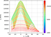 |
Fig. A.3. Same as Fig. A.1, but for the rectification method resimplex3. The respective χ2 = 1217823. |
Appendix B: Supplementary figures
Here we show parameters of the blaze function (Fig. B.1), synthetic spectra of individual components Aa, Ab, B, C (Fig. B.2), the ETVs of ξ Tau for the model with tides (Fig. B.3), and the MCMC analysis for the model without tides (Fig. B.4).
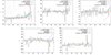 |
Fig. B.1. Parameters of the blaze function as a function of the order r, shown either as discrete values αr, δr, ϵr, θr, γr, or as continuous polynomials α(r), δ(r), ϵ(r), θ(r), γ(r). We show a comparison of two rectification methods: resimplex1 on a set of 10 spectra (black), resimplex1 on a different set of 10 spectra (gray), resimplex2 (blue), resimplex2 with splitting at orders 16, 28, 48 (red). We also show a preliminary fit of black values (green), which served as a starting for resimplex2. The variability of discrete values is substantial, especially for orders r ≳ 50 (Paschen series), but this is suppressed when using polynomials. |
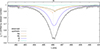 |
Fig. B.2. Synthetic spectra of individual components Aa, Ab, B, C for the model with χ2 = 3639180, in the Hβ line region. |
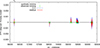 |
Fig. B.3. Same as Fig. 2 for non-zero tides, with revised uncertainties of ETVs of the order of 10−4 d. The total χ2 = 4145. Systematics of ETVs were largely compensated by suitable a value of Δt. |
 |
Fig. B.4. MCMC analysis for the reference model with χ2 = 1553, constrained by SKY, RV, ETV, ECL, SED, SED2 datasets. The corner plot shows uncertainties and correlations of 30 parameters, which were sampled with 64 walkers, 1000 iterations, with 500 burn-in steps. The highest-probability model is plotted (green). Specifically, msum = 9.572 ± 0.023 M⊙, q1 = 0.949 ± 0.001, q2 = 0.851 ± 0.004, q3 = 0.176 ± 0.001, P1 = 7.14730 ± 0.00010 d, log e1 = −2.835 ± 0.014, i1 = 87.050 ± 0.204°, Ω1 = 328.727 ± 0.143°, ϖ1 = 113.833 ± 0.646°, λ1 = 58.676 ± 0.144°, P2 = 145.779 ± 0.005 d, log e2 = −0.682 ± 0.003, i2 = 86.753 ± 0.120°, Ω2 = 328.575 ± 0.133°, ϖ2 = 340.150 ± 0.666°, λ2 = 63.402 ± 0.223°, P3 = 18803.7 ± 68.1 d, log e3 = −0.242 ± 0.001, i3 = −23.899 ± 0.157°, Ω3 = 101.493 ± 0.642°, ϖ3 = 117.655 ± 0.196°, λ3 = 148.337 ± 0.088°, T1 = 10520 ± 39 K, T2 = 10369 ± 77 K, T3 = 14060 ± 107 K, log g1 = 4.366 ± 0.019, log g2 = 4.352 ± 0.015, log g3 = 4.302 ± 0.008, γ = 10.132 ± 0.070 km s−1, d = 65.951 ± 0.112 pc. These 1-σ uncertainties are considered local and small, compared to global ones in Table 1, because of some systematics and tension remained in the model. |
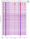 |
Fig. B.5. Comparison of CTIO/CHIRON observed spectra (one per night) with synthetic spectra, for the model with χ2 = 3639180. The fit is acceptable, including the Hα, Hβ wings, with a notable exception of the Hα, Hβ core depths for Aa, Ab components (see red circles for spectra with higher signal-to-noise ratio). |
Appendix C: Supplementary tables
Here we show the journal of photometric observations (Table C.1) and dependent parameters of ξ Tau models (Table C.2)
Journal of photometric observations.
Dependent parameters of ξ Tau models.
All Tables
Best-fit parameters of ξ Tau models. The ‘original’ one is taken from Nemravová et al. (2016), Table 15.
All Figures
|
Fig. 1. Rectification of a CTIO/CHIRON echelle spectrum (ktc00027) in the region of the Hα line (6563 Å), using the resimplex3 method. Top: Synthetic spectra were computed from our model in Table 1, ‘all-data’ column. Four component spectra (Aa, Ab, B, C) and the resulting spectrum are plotted. Second row: Observed spectrum from CHIRON (black), orders r = 39 to 41, and the corresponding blaze function (green). Third row: Rectified spectrum (black), its comparison to the synthetic spectrum (blue), and corresponding residuals (red). The rectification was done with respect to the continuum level, with interpolation of the blaze parameters over wide lines (cyan) and problematic orders, also avoiding locations of the telluric lines (green). Bottom: Residuals plotted separately. |
| In the text | |
|
Fig. 2. Reference model of ξ Tau, showing ETVs (top), eclipse durations (middle), perturbations with respect to a two-body ephemeris (bottom), MOST and TESS observations (blue), model (grey), residuals (red), and, for reference, observed minima (green). The total χ2 = 1553 (see Table 1 for individual contributions). The mean ephemeris used in the bottom panel is P = 7.146665 d, T0 = 2456224.704705. Our model is certainly able to explain the major perturbations, which are substantial (±0.02 d, or ±30 min), but some systematics remain to be explained (up to 0.002 d, or 3 min). |
| In the text | |
|
Fig. 3. Best-fit models of ξ Tau constrained by multi-technique observations for two fixed parameters, the total mass msum and the distance d. The χ2 values (colours) indicate best fit (cyan), good fits (blue), and poor fits (orange); the overall best fit (red) has χ2 = 1661 (unreduced). We tested 121 pairs of parameters and 3000 sequential iterations of simplex, i.e. 3.6 × 10⁵ models in total. Other dynamical parameters (except msum, d) were free; other radiative parameters were fixed (Nemravová et al. 2016). We constrained the model by SKY, RV, ETV, ECL, SED, SED2 data sets; we did not use interferometry (but we used SKY), spectroscopy (but RV), or light curves (but ETV, ECL). We assumed unit weights, except wetv = wecl = 100, because we wanted to exclude all models with incorrect dynamics. The two parameters are often positively correlated (e.g. SKY, VIS, CLO, T3), as predicted (Kepler 1619), but some data sets are distance independent or orthogonal (RV, ETV, SED, SED2), and the model is considered well constrained. After re-convergence (green), the χ2 further decreased to 1553. The Gaia distance of 59.6 pc was excluded. Additionally, VIS, CLO, and T3 were also computed, but their weights were set to zero, otherwise our model would exhibit tension between VIS and CLO. |
| In the text | |
|
Fig. 4. Best-fit model from Fig. 3 with χ2 = 1553 (unreduced). Plots for each data set, SKY, RV, ETV, ECL, VIS, CLO, T3, SED, and SED2, contain observations (blue), synthetic data (yellow), and residuals (red). The best-fit distance is d = 66.0 pc. One can notice some systematics for ETV (see MOST 2017), VIS, or CLO data sets. |
| In the text | |
|
Fig. 5. Same as Fig. 3 but for two different fixed parameters, the effective temperatures T1and T3. This time, light curves (LC) and synthetic spectra (SYN) were included. The overall best fit χ2 = 3639180 (unreduced). One can notice some systematics; for example, there is tension between VIS and CLO, the best ECL is offset, the best SED is offset, and the best SED2 is very offset. |
| In the text | |
|
Fig. 6. Best-fit model from Fig. 5 with χ2 = 3639180 (unreduced). The light curves (LCs) were phased, to show different minima depths (MOST versus TESS). The synthetic spectra (SYN) plot presents only a subset of ten spectra and only the Hβ line region. One can still notice some systematics for ETV (MOST 2017 offset), ECL (TESS offset), VIS (individual observations), CLO (individual observations), SED (overestimated), SED2 (underestimated), or SYN (Aa, Ab line depths are not sufficient). |
| In the text | |
|
Fig. 7. Same as Fig. 3 but for different fixed parameters, i.e., the oblateness, C20, 1, and the tidal time lag, Δt1. For the second component we assumed the same values. The uncertainties of ETVs were revised to 10−4 d. We tested 121 pairs of parameters, 300, 300, and 1000 sequential iterations of simplex: 1.9 × 10⁵ models in total. The parameters of the inner Aa+Ab orbit (plus P2) were free. The best fit is indicated (red) along with a statistically equivalent, close-to-zero C20, 1 solution (green). Zero Δt1 is excluded. |
| In the text | |
|
Fig. 8. Same as Fig. 7 but the parameters of all orbits were free. The solutions differ from Fig. 7 partly because of perturbations by component C. The solutions with low Δt1 ∼ 100 s exhibit a poor fit of eclipse duration (ECL), so the solution with high Δt1 (and zero C20, 1) is still preferred. |
| In the text | |
|
Fig. 9. Same as Fig. 7 but for models with five components (Aa+Ab+B+Ca+Cb). The perturbations and the light-time effect due to Ca+Cb components were stronger. The best-fit solution with low Δt1 ∼ 100 s now exhibits a good fit of eclipse duration (ECL). |
| In the text | |
|
Fig. 10. Angular-momentum vectors of the ξ Tau sub-systems (Aa+Ab, B, C) and their long-term evolution. The coordinates were rotated to the Laplace reference frame, with the z-axis along the total angular momentum, Lsum, of the whole ξ Tau system (in absence of external torques Lsum is constant). The individual contributions were obtained as |
| In the text | |
|
Fig. 11. Same as Fig. 10 but only for three bodies (A, B, C), where A represents Aa+Ab. Without a protection mechanism, the Kozai oscillations were triggered, with a period of ≃11500 y. The angular momenta LB and LC still describe conical surfaces, but now their mutual angle J exhibits large oscillations, which triggers correlated oscillation of eccentricities and inclinations of the inner and outer orbits. |
| In the text | |
|
Fig. 12. Osculating orbital elements of ξ Tau in the course of time, for the model with χ2 = 3639180. The angular elements are expressed in the observer’s reference frame. See the description in the main text. |
| In the text | |
|
Fig. 13. Photocentre motion of the ξ Tau system and its influence on parallax measuments. We plot the orbital motion of individual components Aa, Ab, B, C in the barycentric frame (light gray or coloured, if within the observational timespan of Gaia), the photocentre motion (black), the parallactic motion (gray), the proper motion (light gray), and all contributions with the new parallax π′ = 14.717 mas (cyan). For comparison, we plot all contributions with the old parallax π = 16.791 mas (light cyan) and also the old trajectory from Gaia DR3 (dash-dotted). |
| In the text | |
|
Fig. 14. Periodogram of ξ Tau from the TESS (top) and MOST 2012 (bottom) light curves. We removed eclipses and computed five Fourier transforms (Lenz & Breger 2005), with fitting of frequencies, amplitudes and phases, and subtracting the respective model, ∑iAisin[2π(fit + ϕi)]. For TESS, the dominant frequencies were 1.407, 2.371, 1.421, 2.814, and 0.279 d−1. We note f4 = 2f1 and f5 = 2forb of the inner orbit. For MOST 2012, on the contrary, we found 2.369, 2.216, 0.993, 0.282, and 2.839 d−1. The non-existent 1.407 d−1 frequency is labeled “ftess”. |
| In the text | |
|
Fig. A.1. Redefined blaze function R(λ), according to (Eq. (A.6)), estimated for CTIO/CHIRON spectra. It is plotted in absolute, analog-digital units (adu) and for shifted wavelengths λ − λc, r, for each order r. The rectification method was resimplex1. Colours correspond to χ2 contributions. The total χ2 = 666239 (unreduced) is a measure of correspondence between the rectified observed spectra and the synthetic (rectified) spectra. |
| In the text | |
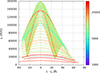 |
Fig. A.2. Same as Fig. A.1, but for the rectification method resimplex2. The respective χ2 = 891923. |
| In the text | |
|
Fig. A.3. Same as Fig. A.1, but for the rectification method resimplex3. The respective χ2 = 1217823. |
| In the text | |
|
Fig. B.1. Parameters of the blaze function as a function of the order r, shown either as discrete values αr, δr, ϵr, θr, γr, or as continuous polynomials α(r), δ(r), ϵ(r), θ(r), γ(r). We show a comparison of two rectification methods: resimplex1 on a set of 10 spectra (black), resimplex1 on a different set of 10 spectra (gray), resimplex2 (blue), resimplex2 with splitting at orders 16, 28, 48 (red). We also show a preliminary fit of black values (green), which served as a starting for resimplex2. The variability of discrete values is substantial, especially for orders r ≳ 50 (Paschen series), but this is suppressed when using polynomials. |
| In the text | |
|
Fig. B.2. Synthetic spectra of individual components Aa, Ab, B, C for the model with χ2 = 3639180, in the Hβ line region. |
| In the text | |
|
Fig. B.3. Same as Fig. 2 for non-zero tides, with revised uncertainties of ETVs of the order of 10−4 d. The total χ2 = 4145. Systematics of ETVs were largely compensated by suitable a value of Δt. |
| In the text | |
|
Fig. B.4. MCMC analysis for the reference model with χ2 = 1553, constrained by SKY, RV, ETV, ECL, SED, SED2 datasets. The corner plot shows uncertainties and correlations of 30 parameters, which were sampled with 64 walkers, 1000 iterations, with 500 burn-in steps. The highest-probability model is plotted (green). Specifically, msum = 9.572 ± 0.023 M⊙, q1 = 0.949 ± 0.001, q2 = 0.851 ± 0.004, q3 = 0.176 ± 0.001, P1 = 7.14730 ± 0.00010 d, log e1 = −2.835 ± 0.014, i1 = 87.050 ± 0.204°, Ω1 = 328.727 ± 0.143°, ϖ1 = 113.833 ± 0.646°, λ1 = 58.676 ± 0.144°, P2 = 145.779 ± 0.005 d, log e2 = −0.682 ± 0.003, i2 = 86.753 ± 0.120°, Ω2 = 328.575 ± 0.133°, ϖ2 = 340.150 ± 0.666°, λ2 = 63.402 ± 0.223°, P3 = 18803.7 ± 68.1 d, log e3 = −0.242 ± 0.001, i3 = −23.899 ± 0.157°, Ω3 = 101.493 ± 0.642°, ϖ3 = 117.655 ± 0.196°, λ3 = 148.337 ± 0.088°, T1 = 10520 ± 39 K, T2 = 10369 ± 77 K, T3 = 14060 ± 107 K, log g1 = 4.366 ± 0.019, log g2 = 4.352 ± 0.015, log g3 = 4.302 ± 0.008, γ = 10.132 ± 0.070 km s−1, d = 65.951 ± 0.112 pc. These 1-σ uncertainties are considered local and small, compared to global ones in Table 1, because of some systematics and tension remained in the model. |
| In the text | |
|
Fig. B.5. Comparison of CTIO/CHIRON observed spectra (one per night) with synthetic spectra, for the model with χ2 = 3639180. The fit is acceptable, including the Hα, Hβ wings, with a notable exception of the Hα, Hβ core depths for Aa, Ab components (see red circles for spectra with higher signal-to-noise ratio). |
| In the text | |
Current usage metrics show cumulative count of Article Views (full-text article views including HTML views, PDF and ePub downloads, according to the available data) and Abstracts Views on Vision4Press platform.
Data correspond to usage on the plateform after 2015. The current usage metrics is available 48-96 hours after online publication and is updated daily on week days.
Initial download of the metrics may take a while.