


| Issue |
A&A
Volume 711, July 2026
|
|
|---|---|---|
| Article Number | A189 | |
| Number of page(s) | 13 | |
| Section | Extragalactic astronomy | |
| DOI | https://doi.org/10.1051/0004-6361/202659329 | |
| Published online | 14 July 2026 | |
Evolution of dust attenuation in star-forming galaxies with UV slope, stellar mass, and redshift out to z∼5
1
Institute of Astronomy, Faculty of Physics, Astronomy and Informatics, Nicolaus Copernicus University, Grudzidzka 5, 87-100, Toruń, Poland
2
Institute for Astronomy, University of Edinburgh, Royal Observatory, Edinburgh, EH9 3HJ, UK
3
National Centre for Nuclear Research, Pasteura 7, 093, Warsaw, Poland
4
Astronomical Observatory Institute, Faculty of Physics and Astronomy, Adam Mickiewicz University, ul. Słoneczna 36, 60-286, Poznań, Poland
★ Corresponding author: This email address is being protected from spambots. You need JavaScript enabled to view it.
Received:
5
February
2026
Accepted:
24
May
2026
Abstract
Context.To set reliable constraints on the dust-obscured portion of star formation across cosmic time, an accurate calibration of the so-called infrared excess (IRX ≡ LIR/LUV) and its dependence on intrinsic galaxy properties is required. While the local IRX-β relation (where Fλ ∝ λβ) has been widely used to correct for the effects of dust absorption and scattering, many recent high-redshift works show significant inconsistencies. They are most likely caused by differences in the assumed attenuation curves, dust temperatures, and galactic star-to-dust relative morphologies.
Aims. We found a dependence of the IRX on the UV slope β, stellar mass M*, and redshift out to z ≃ 5. We also established consistent functional relations that can be used for correcting the UV/optical-selected galaxy samples for the effects of dust absorption.
Methods. This work is based on a K-band selected sample of ∼105 star-forming galaxies detected in the UDS and COSMOS fields. Quiescent sources and known starbursts have been removed, while the IR luminosities were established via stacking in FIR Herschel and JCMT maps. The UV slopes were determined from the spectral energy distribution (SED) fits and stacked IRX values were derived by taking the median of individual IRX measurements in bins of β, M*, and redshift.
Results. While our best-fit IRX-β relation is consistent with a Calzetti-like attenuation curve at β ≳ −1, at bluer values, the IRX appears to increase with redshift due to different mass-completeness limits imposed. When deriving the IRX-β relation in stellar-mass bins, a systematic trend was found, where the effective slope of the attenuation law becomes progressively shallower with increasing mass. We incorporated this into the IRX-β relation through the slope of the underlying reddening law, dA1600/dβ, which is a quadratic function of log(M*/M⊙). Expressing IRX as a function of the stellar mass, we find a tight correlation, with IRX rising monotonically with mass, while exhibiting a clear high-mass turnover at z ≲ 2 − 3, consistent with suppressed cold-gas accretion and dust growth in massive systems.
Key words: galaxies: evolution / galaxies: formation / galaxies: high-redshift / galaxies: ISM / galaxies: star formation
© The Authors 2026
 Open Access article, published by EDP Sciences, under the terms of the Creative Commons Attribution License (https://creativecommons.org/licenses/by/4.0), which permits unrestricted use, distribution, and reproduction in any medium, provided the original work is properly cited.
This article is published in open access under the Subscribe to Open model. This email address is being protected from spambots. You need JavaScript enabled to view it. to support open access publication.
1. Introduction
The accurate determination of the cosmic star-formation rate density (ρSFR) across cosmic time remains a fundamental objective of observational cosmology. To build a complete picture of the star-formation activity in the Universe, it is necessary to account for all the energy produced by young, massive stars. This includes both the direct rest-frame ultraviolet (UV) emission that escapes the host galaxy and the fraction absorbed by the interstellar medium (ISM) and re-emitted at far-infrared (FIR) wavelengths. While this task is relatively straightforward in the Local Universe due to the wealth of the available high-resolution imaging, at high redshifts (z > 2) the impact of the interstellar dust becomes harder to assess (Madau & Dickinson 2014 and references therein).
One common method for quantifying the dust-obscured fraction of the stellar light is based on the so-called IR excess (IRX ≡ LIR/LUV) and its relationship to galaxies’ optical properties, such as the UV slope (β) or the stellar mass (M*). Historically, the relationship between IRX and β has been used as a primary proxy for dust attenuation (e.g., Calzetti et al. 2000; Reddy et al. 2012; Bouwens et al. 2016; Fudamoto et al. 2020b). Originally established by Meurer et al. (1999), this relationship describes a tight empirical correlation for local starburst galaxies, with a relatively flat, Calzetti-like attenuation law assumed, where the reddening of a galaxy’s UV color between the rest-frame 125–250 nm can be used to predict its total dust obscuration. For over a decade, this relation was often used for correcting UV-selected samples at high redshifts. However, with more deep-field surveys producing increasing amount of high-redshift imaging, it became evident that “normal” star-forming galaxies (SFGs) differ significantly from the starburst sequence in terms of the dust content (e.g., Reddy et al. 2010, 2012). These deviations have been suggested to arise from a combination of varying stellar population ages, metallicity effects, and complex dust-to-star geometries that are not accounted for by the local Meurer et al. (1999) data (e.g., Narayanan et al. 2018; Salim & Narayanan 2020).
The high-resolution imaging produced by the Atacama Large Millimeter/submillimeter Array (ALMA) has further complicated this picture. Initial FIR observations of Lyman-break galaxies (LBGs) at z ∼ 5 − 6 reported surprisingly low IRX values (Capak et al. 2015; Bouwens et al. 2016), representing a departure from the local Calzetti-like attenuation law typically applied to star-forming systems. This suggested that high-redshift galaxies are potentially more consistent with the Small Magellanic Cloud (SMC)-like extinction law. In addition, wrongly measured or assumed temperature of the interstellar dust (Td) was also shown to play a role in the derived values of the IR luminosities. A number of works established Td to be an increasing function of redshift (e.g., Viero et al. 2022; Ismail et al. 2023; Koprowski et al. 2024), with the apparent “IRX deficit” potentially being an artifact of underestimating the FIR luminosity of warm-dust systems.
Furthermore, the IRX–β relationship has recently been found to also depend on the stellar masses of the galaxy samples (Álvarez-Márquez et al. 2019; Bouwens et al. 2020). It has been found that while low-mass systems at high redshifts appear “IR-faint” for a given value of beta, more massive galaxies, log(M*/M⊙) > 10, are often consistent with the local Calzetti-like attenuation curves. This mass dependence suggests that as galaxies grow, they rapidly accumulate dust and develop the complex, multi-component ISM structures seen in local starbursts (e.g., van der Wel et al. 2025; Gebek et al. 2025; Lisiecki et al. 2025). Recent JWST observations (e.g., Fisher et al. 2025; Shivaei et al. 2026) further indicate that the scatter in the IRX-β plane is amplified by so-called bursty star-formation histories, where high UV luminosities can become “decoupled” from the dust-obscured regions, resulting in dusty sources being characterized by the relatively blue values of the UV slope.
Beyond the complications related to the physical evolution of galaxies, a significant challenge lies in the selection of both rest-frame UV/optical and FIR-based samples. Most high-redshift ALMA studies, for instance, are biased toward the most IR-luminous sources, potentially missing the “normal” population of star-forming galaxies, while samples selected at the rest-frame UV/optical bands are often incomplete in terms of the stellar mass. To overcome this, we utilized a K-band selected sample of approximately 100,000 galaxies from the UKIDSS Ultra Deep Survey (UDS) and COSMOS fields, covering a combined area of nearly 2 deg2 (McLeod et al. 2021). To reach beyond the detection limits of typical FIR observations, we resorted to a well-known method of stacking. This approach is critical for ensuring mass completeness and accounting for the selection effects that often plague individual FIR detections studies. By stacking individual IR excess values of galaxies in distinct UV slope, stellar mass, and redshift bins, we were able to establish a consistent relationship between the IRX, UV slope, stellar mass, and redshift for star-forming galaxies out to z ∼ 5.
This paper is structured as follows. In Section 2 we describe the data used in this work. The star-forming galaxies’ sample selection process and methods used to derive the physical properties and the stacked IRX values are presented in Section 3. In Section 4 the results are presented and discussed, where the high-redshift IRX-β relation is derived in Section 4.1, the stellar mass dependence through the slope of the reddening law is introduced into the IRX-β relationship in Section 4.2, followed by the comparison with recent literature in Section 4.3. The IRX-M* function and its evolution with redshift is presented, discussed, and compared with other studies in Sections 4.4 and 4.5. We present a summary in Section 5. Throughout the paper, we use the Chabrier (2003) stellar IMF with an assumed flat cosmology of Ωm = 0.3, ΩΛ = 0.7, and H0 = 70 km s−1 Mpc−1.
2. Data
2.1. Optical/near-IR catalogs
To determine how the IRX varies across cosmic time, we stacked the optical/near-IR star-forming galaxies’ samples of the UKIDSS Ultra Deep Survey (UDS) and COSMOS fields (McLeod et al. 2021) in the FIR Herschel and James Clerk Maxwell Telescope (JCMT) maps. The details of the data used, the selection process, catalog construction, and the determination of photometric redshifts and stellar masses are presented in McLeod et al. (2021), with a short summary given below.
The UKIDSS UDS field (Lawrence et al. 2007) includes UDS DR11 imaging (Almaini et al., in prep.) in the near-IR JHK bands, Y-band imaging from the VISTA VIDEO DR4 (Jarvis et al. 2013), UV imaging in u*-band from CFHT MegaCam (Gwyn 2012), optical imaging in BVRiz′ from Subaru Suprime-Cam (Furusawa et al. 2008), and the mid-IR (MIR) Spitzer IRAC imaging in 3.6 μm and 4.5 μm, combining the SEDS (Ashby et al. 2013), S-CANDELS (Ashby et al. 2015), and SPLASH (PI Capak; see Mehta et al. 2018) programs. The effective area of the overlapping UDS imaging was 0.69 deg2, after masking for bright stars. For the COSMOS field, near-IR YJHKs imaging from UltraVISTA DR4 (McCracken et al. 2012) with UV/optical u*griz imaging from the CFHTLS-D2 T0007 data release are combined. As with the UDS, the data also includes the Spitzer IRAC imaging available in 3.6 μm and 4.5 μm, covering the area of 0.86 deg2.
The optical/NIR data available for each galaxy were fit with a number of spectral energy distribution (SED) codes, where the final redshift was taken to be the median of individual values, zmed. The precision was assessed using the available spectroscopic data, with σz values, defined as 1.483 × MAD(dz), where MAD is the median absolute deviation and dz = (zmed − zspec)/(1 + zspec), for the COSMOS and UDS fields, found to be equal to 0.019 and 0.022, respectively (McLeod et al. 2021).
Stellar masses were measured for each object by fixing the photometric redshift to zmed, and refitting the SED using LEPHARE with the Bruzual & Charlot (2003) library, a Chabrier (2003) IMF, a Calzetti et al. (2000) dust attenuation law, and IGM absorption as in Madau (1995). The resulting values were checked against masses found by the CANDELS team, where a tight 1:1 relation and a typical scatter of ±0.05 dex was found.
2.2. Far-infrared
We used two different stacking procedures. For the stacked IRX values in bins of UV slope, stellar mass, and redshift, the FIR flux densities in the COSMOS and UDS fields were extracted using the SCUBA-2 Cosmology Legacy Survey (S2CLS; Geach et al. 2017) 850 μm imaging, as explained in Section 3.4. To determine the functional form of the IRX-β relationship, however, our sample was additionally stacked in the Herschel (Pilbratt et al. 2010) Multi-tiered Extragalactic Survey (HerMES; Oliver et al. 2012) and the Photodetector Array Camera and Spectrometer (PACS; Poglitsch et al. 2010) Evolutionary Probe (PEP; Lutz et al. 2011) maps obtained with the Spectral and Photometric Imaging Receiver (SPIRE; Griffin et al. 2010) and PACS instruments (Section 4.1).
3. Methods
3.1. Sample selection
We binned our data in equal redshift intervals spanning 0.5 < z < 5.0 with a step size of Δz = 0.5, with the exception of the highest-redshift bin, where the bin width was set to Δz = 1.0 to improve the detection rate. For the analysis of the IRX-β relation, we set the lowest redshift to 2.0 since, at lower values, the available photometry does not cover the rest-frame UV slope interval of 125–250 nm. Additionally, we restricted our sample to sources exceeding the 90% stellar mass completeness limit established by McLeod et al. (2021). This results in lower mass thresholds of log(M*/M⊙) = [9.50, 9.50, 9.50, 9.50, 9.75, 9.75, 10.00, 10.25] across the respective redshift bins defined by z = [0.5, 1.0, 1.5, 2.0, 2.5, 3.0, 3.5, 4.0, 5.0], with a total of 135596 galaxies.
Quiescent galaxies were excluded based on the NUVrJ color-color selection criteria of Ilbert et al. (2013), expressed as
 (1)
(1)
where the NUV, r, and J AB magnitudes were determined from the SED fitting (see Section 3.2). This method separates sources whose reddening results from the aging of the stellar population (i.e., quiescent galaxies) from the dusty star-forming sample. The NUVrJ color-color selection was limited to redshifts less than 4, as the rest-frame J-band becomes progressively difficult to trace at higher redshifts based on the available photometry, with a total of 18958 (14%) sources identified as quiescent.
Similarly to Koprowski et al. (2024), we also identified and removed 479 starburst galaxies, using the ALMA-selected samples in the COSMOS (Liu et al. 2019) and UDS (Stach et al. 2019) fields, with stellar masses and SFRs from Liu et al. (2019) and Dudzevičiūtė et al. (2020), respectively. Following Elbaz et al. (2018), starbursts were defined as galaxies with SFR/SFRMS > 3, with SFRMS being the corresponding main-sequence value (Koprowski et al. 2024).
3.2. SED fitting
A SED fitting was performed to determine the rest-frame NUV, r, and J absolute magnitudes used for quiescent galaxies selection (Eq. 1), UV slopes and UV luminosities necessary for the derivation of the stacked IRX values and the IRX-β relationship functional form parameters (Section 4.1). We used the Code Investigating GALaxy Emission (CIGALE; Boquien et al. 2019), with the stellar models of Bruzual & Charlot (2003), Chabrier (2003) initial mass function, Calzetti et al. (2000) dust attenuation law, and the IGM absorption of Meiksin (2006). Simple exponential star-formation history models, SFH ∝ exp(−t/τ), were assumed, with τ values of 0.1, 0.3, 1, 2, 3, 5, 10, and 15 Gyr and the dust attenuation, AV, ranging between 0 and 2.8 in steps of 0.05. The NUVrJ magnitudes and the UV luminosities were found for each source by CIGALE from the best-fit SEDs. The procedure for deriving the UV slopes is described in Section 3.3, while the determination of the IRX-β relationship functional form parameters is explained in Section 4.1.
3.3. UV slopes
A number of methods have been used for determining the UV spectral slope, β, a comprehensive review of which is presented in Rogers et al. (2013). Originally, Meurer et al. (1999) calculated β by fitting a power-law function to the ten continuum rest-frame 125–250 nm bands of Calzetti et al. (1994). Most often, however, only a few photometric points are available in this wavelength range; hence, the resulting β’s are burdened with significant uncertainties. As explained by McLure et al. (2018), these uncertainties can bias the stacked values of the IRX, flattening the corresponding IRX-β relationship. Therefore, we derived the UV slopes by fitting the power-law function to the best-fit SEDs in the rest-frame wavelength range of 125 − 250 nm, where Sλ ∝ λβ. As recently shown by Morales et al. (2024), SED-based values exhibit lower scatter and reduced biases than those derived from photometric power-law fitting.
To estimate the UV slope uncertainties for each source, the photometry was randomly sampled from normal distributions, with the means and standard deviations corresponding to the catalog values and their associated errors and the resulting value of βi derived from the best-fit SED. The procedure was repeated 1000 times and the final errors were taken to be the standard deviations of the individual values of βi. Due to the diminishing quality of the photometry with redshift, the mean values of βi end up increasing from 0.15 at z ∼ 2 to 0.55 at z ∼ 5.
3.4. Stacked IRX values
For about 600k star-forming galaxies in our optical/near-IR catalogs, only ∼2000 sources were directly detected in the S2CLS 850 μm survey (Geach et al. 2017). To obtain reliable estimates of the IR luminosity, and hence the IRX, we, therefore, resorted to the well-known method of stacking (e.g., Tomczak et al. 2016; Leslie et al. 2020; Mérida et al. 2023; Koprowski et al. 2024). Because it is not clear how does LIR couple with LUV, the stacked values of the IRX were taken to be equal to the median of the individual values of the IR excess found for each source in the stack. For this to work, individual values of both, the UV and the IR luminosity for each source had to be found. While the UV luminosities were established from the SED fitting to the available UV/optical photometry, as described in Section 3.2, the determination of individual values of LIR is difficult, due to the relatively shallow depth of the FIR observations. The FIR Herschel and JCMT SCUBA-2 flux densities extracted at each source’s position are well below the noise level and to extract the IR luminosities, we first need to make an assumption on the dust temperature. Therefore, to derive stacked IRX values in bins of β, M*, and redshift, we relied on a single FIR photometry band. Specifically, we extracted the SCUBA-2 850-μm flux density at each source’s position, converted it to IR luminosity, and divided it by the corresponding UV luminosity. Then, LIR was found by integrating the best-fit dust emission curve of Casey (2012) between 8–1000 μm rest frame, with the emissivity and the MIR power-law slope set to 1.96 and 2.3, respectively, as per recommendations of Drew & Casey (2022). To determine the dust temperature, we applied the Td–z relation from Koprowski et al. (2024), which was derived from a stacking analysis of the exact same sample used in this work. In each bin, the corresponding stacked values of the UV slope, stellar mass, and redshift were also derived by taking the median of all the individual numbers.
The impact of redshift and stellar-mass uncertainties on the stacked values of the IRX, β, M*, and redshift was quantified using a bootstrap method. At each iteration, a mock catalog was generated by randomly drawing, with replacement, a set of sources from the original mass-complete dataset, for which a stacked value was found, following the procedure described above. The process was repeated 1000 times and the errors, δbootstrap, were then taken to be the median absolute deviation of the resulting simulated values. In addition, to account for uncertainties in the UV luminosity and UV slope, we performed simple Monte Carlo simulations. In each of the 1000 runs, the values of LUV and β were randomly drawn from Gaussian distributions with standard deviations set to their respective 1σ uncertainties. The corresponding errors, δMC, were taken to be equal to the median of the individual values found in each run. The final uncertainties were then determined, where
 (2)
(2)
4. Analysis and discussion
4.1. IRX-β in bins of UV slope
To find the evolution of the IR excess with the UV slope and redshift, we stacked our mass-complete sample following the procedure explained in Section 3.4. The redshift and β bins and the mass-completeness limits, adopted from McLeod et al. (2021), with the corresponding IRX-β median values are summarized in Table A.1 and plotted in Figure 1 as color points with error bars.
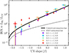 |
Fig. 1. IRX-β relationship for 2.0 < z ≤ 5.0 sample studied in this work. The color points with error bars show the stacked values of the IRX in bins of β, summarized in Table A.1. The black solid line represents the best-fit functional form (Equation 9), with dA1600/dβ = 1.97 being consistent with the attenuation curve of Calzetti et al. (2000). The scatter at β ≲ −1 is caused by different stellar mass completeness limits imposed at each redshift bin (see Section 4.1 for details). For reference, the SMC curve is plotted in dashed line. |
The functional form was adopted from Meurer et al. (1999) via
 (3)
(3)
where A1600 is the attenuation at the rest-frame 1600Å and B is the ratio of two correction factors:
 (4)
(4)
Since, in the original work of Meurer et al. (1999), the FIR luminosity, measured using IRAS data, was defined as LFIR = 1.25(L60 + L100) and the UV luminosity was determined at the rest-frame 1600 Å, corrections were required to convert into bolometric luminosities. In this work, the IR luminosity is found by integrating the best-fit dust emission curve between 8–1000 μm (Section 3.4), so the FIR correction factor is by definition equal to 1. BC(1600), on the other hand, can be found once the intrinsic stellar emission curve is known. The attenuation at the rest-frame 1600 Å is defined as
 (5)
(5)
with βobs and βint being the UV slopes of the observed and the intrinsic stellar emission spectra, respectively.
To establish the best-fit functional form of the IRX-β relation (i.e., the best-fit values of BC(1600) and A1600), it is first necessary to find the underlying shapes of the intrinsic and observed UV-FIR SEDs. Following previous works (e.g., McLure et al. 2018; Koprowski et al. 2018) and our stacked results given in Figure 1, we assumed the IRX-β relation not to evolve significantly with redshift. Therefore, we derived our SEDs for the whole 2.0 < z < 5.0 sample combined. To deal with nondetections, in the UV/optical bands, we adopted median stacked values. For the FIR Herschel and JCMT SCUBA-2 bands, a stacking analysis was performed, following the procedure explained in Section 3.2 of Koprowski et al. (2024). In brief, an inverse-variance weighting stacking method was utilized to derive average fluxes in a given band. For each source a square stamp was extracted with a side length approximately three times the full width at half maximum (FWHM) of the corresponding beam. The average stacked FIR flux densities were subsequently determined by applying nonlinear least squares best fits to the resulting light profiles. Because source clustering contributes significantly to the mean flux in the larger Herschel SPIRE bands, a double Gaussian profile was often utilized to accurately model and subtract this background contamination. Finally, the uncertainties on these stacked FIR fluxes were estimated using a bootstrapping method that incorporated instrumental noise and functional fit errors. The corresponding best-fit observed and intrinsic SEDs were then found by fitting to the stacked UV-FIR photometry using CIGALE, as explained in Section 3.2, with the slope of the dust reddening law, dA1600/dβ, set as a free parameter. The intrinsic stellar emission curve was then used to calculate the intrinsic UV slope and the bolometric correction factor, BC(1600) expressed as
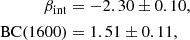 (6)
(6)
with the resulting best-fit IRX-β relationship functional form plotted as black solid line in Figure 1. Because our sample contains significantly more sources at lower redshifts, stacking all galaxies across the 2.0 < z < 5.0 range biases the resulting fits toward low-z data. However, when stacking was performed in separate redshift bins, the derived IRX-β relations showed only a slight variation at β < −2.0, with the lower-redshift fits yielding slightly higher intrinsic UV slopes and BC(1600) values, reflecting the older average ages of their underlying stellar populations.
To estimate the errors, we performed simple Monte Carlo simulations. In each of 1000 realizations, the photometry was randomly sampled from the Gaussian distribution with the means and standard deviations equal to the catalog’s values and their errors, respectively. The best-fit SEDs were found and the bolometric correction, BC(1600), and βint calculated for each run. The final errors were then set to be equal to the median of all the individual values. The best-fit slope, dA1600/dβ = 1.97, is consistent with the Calzetti et al. (2000) reddening law, assuming
 (7)
(7)
for the Calzetti attenuation law and SMC extinction curve, respectively (McLure et al. 2018). Accordingly, our best-fit IRX–β relation is hereafter referred to as a Calzetti-like attenuation law.
Figure 1 shows that at β > −1.0 our IRX-β relationship is in agreement with the Calzetti et al. (2000) attenuation curve across all redshift bins. At bluer β’s, however, the values of the IRX seem to be increasing with redshift. In Figure 2 the median values of the UV slope and stellar mass, corresponding to the stacked data of Figure 1, color-coded with redshift are plotted. The green background image shows a 2D histogram of the βobs–M* distribution, with the black contours corresponding to the values of 1, 10, 100, and 1000. We can see that at bluer β values, the median stellar masses are significantly larger at higher redshifts, reflecting different stellar mass completeness limits imposed in each redshift bin (Table A.1). This aligns with recent results indicating that IRX correlates with stellar mass, such that at fixed β, systems with higher stellar masses exhibit larger values of the IR excess (e.g., Álvarez-Márquez et al. 2019; Bouwens et al. 2020). To investigate this further, we stacked individual values of the IR excess in bins of the stellar mass, as described in the next section.
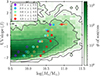 |
Fig. 2. Relationship between the UV slope and the stellar mass for the sample presented in Figure 1. Green background image shows a 2D histogram of the β–M* distribution, with 1, 10, 100 and 1000 sources contours displayed with black curves. It can be seen that due to different mass-completeness limits imposed at each redshift bin (Table A.1), the median stellar masses at bluest β bins increase with redshift, which in turn drives the scatter in Figure 1 (see Section 4.1 for details). |
4.2. IRX-β in bins of stellar mass
Following the procedure explained in Section 3.4, the stacked median values of the IR excess were found in bins of the stellar mass for all the sources between redshifts 2.0 and 5.0, where in each stellar mass bin the corresponding UV slope was assumed to be the median of all the individual β’s. The results of this exercise are presented in Figure 3 with black open circles and summarized in Table 1. For reference, the best-fit functional form of the IRX-β relation found in Section 4.1 (consistent with the Calzetti et al. 2000 curve) and the SMC-like relation are plotted as black solid and dashed lines, respectively. It can be clearly seen that the position of a given IRX-β stacked data point relative to the best-fit relation correlates with the median stellar mass.
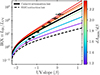 |
Fig. 3. IRX-β relationship in bins of stellar mass. The black circles show the stacked data (Table 1), with a clear correlation between the stellar mass and the slope of the reddening law, dA1600/dβ. Adopting Equation (9), with dA1600/dβ set as free parameter, best-fit values for the reddening slope were found (last column in Table 1), with the corresponding correlation with the stellar mass derived in Section 4.2 and plotted in Figure 4. For reference, this work’s best-fit relationship (consistent with the Calzetti curve), together with the SMC curve are plotted in solid and dashed lines, respectively. |
As explained in a number of recent works (e.g., Narayanan et al. 2018; Koprowski et al. 2018; Salim & Narayanan 2020), the scatter in the IRX-β plane is mainly caused by the variations in the slopes of the underlying attenuation laws, where galaxies affected by flatter (grayer) curves are shifted towards bluer UV slopes. Salim & Narayanan (2020) show that the attenuation curves slopes correlate strongly with effective optical opacity (i.e. the dust column density), with dusty and more massive galaxies having, on average, grayer curves. They attribute this relationship primarily to the combined effects of radiative transfer processes (scattering and absorption) and local geometry (clumpiness of dust). In this framework, a fraction of the rest-frame UV light, originating from young massive stars, escapes the galaxy through gaps in the dust distribution and via scattering processes, causing the effective attenuation curve to flatten.
It has been shown that galaxies at high redshifts exhibit a large variety of dust attenuation laws (e.g., Kriek & Conroy 2013; Lo Faro et al. 2017; Salmon et al. 2016; Cullen et al. 2018). Álvarez-Márquez et al. (2019) investigated a sample of high-redshift LBGs and found more massive sources to be affected by grayer attenuation curves. A similar trend was found by Bouwens et al. (2020). More recently, Shivaei et al. (2026) investigated a spectroscopic sample from three JWST/NIRCam grism surveys and found the slopes of the attenuation curves to become shallower at higher values of the dust attenuation. Given that the dust attenuation is positively correlated with the stellar mass (i.e. more massive galaxies tend to be more dusty; Figure 2 and also McLure et al. 2018; Bouwens et al. 2020), higher mass sources are systematically expected to be characterized by grayer attenuation curves.
Therefore, we proceeded to establish the functional form of the relationship between the stellar mass and the slope of the underlying attenuation law using data from Figure 3. For practical reasons, the attenuation curve for a given stellar mass bin is quantified with the dust reddening slope of Equation (5), dA1600/dβ. A steeper attenuation curve leads to greater relative attenuation toward the edges of the UV wavelength range over which the UV slope β is measured (i.e., 125–250 nm in the rest frame). That means that for a fixed attenuation, the steeper curve will produce redder β, shifting the galaxy to the right on the IRX-β plane. Consequently, steeper attenuation curves cause β to redden more rapidly as attenuation increases, giving rise to shallower reddening slopes, dA1600/dβ.
Assuming the median intrinsic stellar SED parameters, BC(1600) and βint, found in Section 4.1 for our 2.0 < z ≤ 5.0 sample, dA1600/dβ was established for each IRX-β stacked point in Figure 3 from Equation 3 using the χ2 minimization method. The resulting values are summarized in Table 1 and plotted in Figure 4 with open circles, with the corresponding functional forms of the IRX-β relation depicted in Figure 3 with solid color lines. The correlation between the slope, dA1600/dβ, and the stellar mass was then found using the χ2 minimization method (solid curve in Figure 4), where:
 (8)
(8)
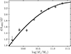 |
Fig. 4. Relationship between the dust reddening slope, dA1600/dβ, and the stellar mass for the sample plotted in Figure 3, where a clear correlation can be seen, with more massive systems being characterized by flatter attenuation curves. The functional form of the relation is derived and discussed in Section 4.2 and summarized in Equation (9). |
with ℳ = log(M*/M⊙) and the errors estimated from the corresponding co-variance matrix. Therefore, the IR excess becomes a function of both the UV slope and the stellar mass, where the later enters the equation through its effect on the slope of the reddening law, dA1600/dβ, with the corresponding functional forms summarized in Table 2. The comparison between the functional form found in this work and the ones determined in Álvarez-Márquez et al. (2019) and Bouwens et al. (2020) are presented in Sections 4.4 and 4.5.
Functional form of the IRX-β-M*-z relationship.
4.3. IRX-β – comparison to previous studies
We plot our stacked data in Figure 5. The gray circles represent median values of the IR excess resulting from stacking all the sources between redshifts 2.0 and 5.0 (Table A.2), adopting stellar mass limits from Table A.1. For reference, this work’s best-fit relationship (consistent with the Calzetti curve), together with the SMC curve are plotted in solid and dashed lines, respectively. It can be seen that our median data is still slightly below the best-fit curve at blue UV slopes. This is caused by the variations in the corresponding stellar masses, with bluer bins having slightly lower median values of M*.
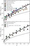 |
Fig. 5. IRX-β relationship derived for the 2.0 < z ≤ 5.0 sample of this work (gray circles; Table A.2). Top panel. Our median data lying slightly below the best-fit curve at blue UV slopes is driven by variations in the corresponding median stellar masses. We compare our data with the recent literature results of Heinis et al. (2013), Reddy et al. (2018), McLure et al. (2018), Koprowski et al. (2018), Álvarez-Márquez et al. (2019), Fudamoto et al. (2020b) and Bouwens et al. (2020). For reference, this work’s best-fit relationship and the SMC-like curve are plotted in solid and dashed lines, respectively. Bottom panel. To investigate the literature scatter, we highlight how varying data treatment methodologies alters our results (gray circles). Adopting a dust temperature of Td = 40 K with a restricted stellar mass of log(M*/M⊙)∼10.5 (green squares), or deriving UV slopes via photometric power-law fitting instead of best-fit SEDs (red crosses), radically changes the shape and normalization of the relation, mirroring the scatter seen in the top panel. See Section 4.3 for details. |
For comparison, in the top panel of Figure 5, we plot the recent literature results of Heinis et al. (2013), Reddy et al. (2018), McLure et al. (2018), Koprowski et al. (2018), Álvarez-Márquez et al. (2019), Fudamoto et al. (2020b) and Bouwens et al. (2020). The stacked data found in this work seem to be in a reasonable agreement with the works of McLure et al. (2018), Koprowski et al. (2018), Álvarez-Márquez et al. (2019) and Fudamoto et al. (2020b), with the slightly elevated values found in Koprowski et al. (2018) most likely caused by the higher dust temperature assumed when deriving their IR luminosities. The numbers presented in Heinis et al. (2013), Reddy et al. (2018) and Bouwens et al. (2020) are slightly below our stacked data. However, due to the variety of methods employed to measure both UV slopes and IRX, the direct comparison between these works is difficult.
The discrepancies between different data sets can be attributed to several methodological choices. These factors include the techniques used to calculate UV slopes, the procedures for de-blending FIR flux densities (particularly in the low-resolution Herschel SPIRE bands), the assumed profiles of dust emission curves, the specific stacking methods applied, and the apparent dependence of IRX values on stellar mass. We illustrate the effects that some of these choices have on the resulting IRX-β relation in the bottom panel of Figure 5. The gray circles, as in the top panel, depict the results of this work. Limiting our sample to sources with the stellar mass of log(M*/M⊙)∼10.5 and setting the dust temperature to the value adopted in Koprowski et al. (2018) of Td = 40 K, our stacking procedure produces the results presented with green squares. On the other hand, when the UV slopes are derived by fitting a power-law to the available photometry between rest-frame 125–250 nm (as opposed to fitting to the best-fit SEDs), we can see the resulting relationship to flatten with β, consistent with the findings presented in McLure et al. (2018). Variations in the assumed dust temperature, stellar mass range, and the method of deriving the UV slope alone can produce discrepancies (0.5 dex at blue end to ∼1 dex at red end), that are similar in magnitude to the ones seen in the top panel of Figure 5.
4.4. IRX-M*
Since measurements of the UV slope, β, are often burdened with significant uncertainties, causing additional scatter in the corresponding IRX values, it is often preferable to express the IR excess as a function of stellar mass. Therefore, we stacked our full 0.5 < z ≤ 5.0 sample in bins of redshift and M*, as summarized in Table A.3, with the resulting median values plotted in Figure 6 with color points. To find the functional form, we started with the IRX-β relationship found in Section 4.1 (Equations (9) summarized in Table 2), with the functional form of the stellar mass evolution of the reddening law, dA1600/dβ, found in Section 4.2 (Equations (10) summarized in Table 2). To express the IRX as a sole function of stellar mass, we converted the observed UV slope, βobs, into stellar mass, M*. This was done using data corresponding to the stacked points of Figure 3, plotted as black open circles in the top panel of Figure 7, by fitting a Gaussian function (black solid line in Figure 7), using nonlinear least squares with the errors estimated from the corresponding co-variance matrix. The resulting relation can be written as
 (12)
(12)
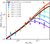 |
Fig. 6. IRX values median-stacked in bins of M* and redshift (color points with error bars; Table A.3). The black line shows the best-fit functional form for the 2.0 < z ≤ 5.0 sample of Figure 3, while the color solid lines depict the functional forms found at the individual redshift bins, as explained in detail in Section 4.4. |
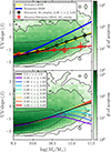 |
Fig. 7. The relationship between the observed UV slope and stellar mass for the 2.0 < z ≤ 5.0 sample of this work. Green background image represents a 2D histogram of the β–M* distribution, with 1, 10, 100 and 1000 sources contours displayed with thin black curves. Top panel. Black circles with error bars show median values of β in bins of M* (Table 1), with the thick black solid curve depicting the best-fit functional form of Equation (12). For comparison, the relationships found in McLure et al. (2018), Álvarez-Márquez et al. (2019) and Bouwens et al. (2020) are shown. Bottom panel. Black curve as in the top panel with the color curves determined for individual redshift bins, following the procedure explained in Section 4.4. |
with ℳ = log(M*/M⊙) and
 (13)
(13)
For comparison, in the top panel of Figure 7, the similar relationships found in McLure et al. (2018), Álvarez-Márquez et al. (2019) and Bouwens et al. (2020) are plotted with yellow, red and blue solid lines, respectively. An excellent agreement between our relationship and the one found in McLure et al. (2018) can clearly be seen. The results of Álvarez-Márquez et al. (2019) are based on a sample of 2.5 < z < 3.5 COSMOS field Lyman Break Galaxies. Since LBGs are selected at the rest-frame UV bands, a fraction of red sources will likely be missed, underestimating the resulting stacked values of the UV slopes. Data investigated in Bouwens et al. (2020), on the other hand, shows elevated β’s at high stellar masses. The source of this inconsistency can be attributed to a slightly different method of deriving the best-fit β–M* relation. In this work, the stacked points in the top panel of Figure 7 were found by taking median values of individual UV slopes in each stellar mass bin, with the best-fit function found from nonlinear least squares (similarly to McLure et al. 2018). In Bouwens et al. (2020), however, the number of sources on each side of the best-fit function was minimized, which produces slightly different results.
By combining Equation (12) with Equations (9) and (10), we obtained the best-fit IRX–M* relationship shown as the black solid line in Figure 6. While it is in agreement with the low-mass stacked data, at higher stellar masses large inconsistencies can clearly be seen. Moreover, the disagreement between the best-fit function and the stacked data seems to increase towards lower redshifts, where the IRX-M* data exhibits a clear turnover. This behavior, which has been detected in previous works (e.g., Whitaker et al. 2014; Pannella et al. 2015), can also be seen in the shape of the star-forming galaxies main sequence (e.g., Tomczak et al. 2016; Popesso et al. 2023; Koprowski et al. 2024). As discussed by Daddi et al. (2022), the turnover in the star-forming main sequence can be caused by phasing out of the cold gas accretion. At this turnover mass, supersonic shocks heat infalling molecular gas and halt cold accretion, effectively starving the galaxy of the fuel needed for sustained, dust-obscured star formation. Since the cold gas accretion is more efficient at higher redshifts, through cold collimated streams traveling along the dark matter filaments, the turnover of the main sequence, and hence the IR excess, shifts towards higher masses at high redshifts, consistent with the Figure 6 data.
The decreasing IRX past the turnover stellar mass indicates that during this starvation phase, the dust-obscured star formation (LIR) undergoes a more rapid reduction relative to the unobscured star formation (LUV). This is because the IR luminosity predominantly traces the youngest massive stars (≲10 Myr) deeply embedded within dense molecular birth clouds, while the unobscured UV luminosity is sensitive to slightly older stellar populations (up to ∼100 Myr) residing in the more diffuse interstellar medium (e.g., Calzetti et al. 2010; Kennicutt & Evans 2012). At the turnover mass, when supersonic shocks heat the incoming gas, the dense molecular reservoirs are rapidly consumed by star formation or dispersed by feedback, decreasing LIR. The UV emission from longer-lived stars; however, persists, resulting in the rapid decline of the corresponding IRX. As the lack of new gas prevents the further accumulation of dust in these massive systems, we expect this decrease in the IRX to be accompanied by a “blueing” of the corresponding UV slope.
Therefore, we would expect the β-M* relation of Figure 7 to also exhibit a turnover at high stellar masses, mimicking the behavior of the IRX-M* stacked data plotted in Figure 6. Since UV slopes cannot be reliably established using our data at redshifts ≲2, where the IRX-M* turnover is most prominent, we derived the corresponding redshift evolution of the β–M* relation indirectly. IRX-M* relation of this work is derived from the best-fit IRX-β curve (Eq. (9)), with the stellar mass evolution of the reddening law given by Eq. (10), and β translated into M* using the appropriate form of the β–M* relationship. Motivated by the arguments presented above, we assume that the position and redshift evolution of the high-mass IRX-M* turnover is driven by the evolution of the corresponding β–M* curve. Therefore, we fit the stacked IRX-M* data (color points in Figure 6) with Equations (9) and (10), allowing the β–M* relation of Eq. (12) to vary. The derived best-fit evolution for the free parameters of the β–M* function, found using nonlinear least squares, is given by
 (14)
(14)
which we summarized in Equation (11) of Table 2 and plotted in the bottom panel of Figure 7 with color solid lines. The corresponding evolution of the best-fit IRX-M* relationship for our stacked median data are depicted with solid color lines in Figure 6. Because our relation is derived from stacked measurements, the small uncertainties on our best-fit β–M* relation parameters represent the precision of the median relation. Individual galaxies, however, exhibit a substantial intrinsic physical scatter of σβ,intr ≈ 0.3 at log(M*/M⊙) = 9.5 increasing to σβ,intr ≈ 0.7 at log(M*/M⊙) = 11.5 around this median track.
It is also important to consider whether alternative factors, such as variations in the dust temperature (Td) or dust SED, could be responsible for the high-mass IRX turnover. In this work, a redshift-dependent Td relation from Koprowski et al. (2024) was adopted, with no stellar mass dependence at a given redshift. However, the dust temperature was found to increase with the specific SFR (e.g., Magnelli et al. 2014; Liang et al. 2019). Because the sSFR for star-forming galaxies with masses above the turnover mass decreases, their dust temperatures are expected to be lower than the average population. As we derived our IRX values from the 850 μm flux density on the Rayleigh-Jeans tail of the dust emission curve, the LIR is highly sensitive to the assumed temperature. Applying a more realistic, mass-dependent (colder) Td to the highest-mass bins would result in lower extrapolated LIR (and IRX) values. Therefore, our assumption of a mass-independent Td provides a conservative upper limit on the corresponding values of the IRX. Assuming lower Td at high-mass end would cause the observed IRX turnover to become even more pronounced.
4.5. IRX-M* and comparisons to previous studies
The comparison of our data with the recent literature results of Whitaker et al. (2014), Heinis et al. (2014), Pannella et al. (2015), McLure et al. (2018), Koprowski et al. (2018), Álvarez-Márquez et al. (2019), Bouwens et al. (2020) and Fudamoto et al. (2020a) is shown in Figure 8. Our 0.5 < z ≤ 5.0 median-stacked values are presented with black filled circles, with the best-fit functional forms, produced by combining Equations (9), (10) and (11) (summarized in Table 2) depicted with black solid lines. A good agreement with most of the works can be seen, with the exception of the low-redshift Whitaker et al. (2014) and Heinis et al. (2014) data and the results of Álvarez-Márquez et al. (2019) and Fudamoto et al. (2020a). A clear high-mass turnover at low redshifts, discussed in previous section, was also detected in the works of Whitaker et al. (2014), Heinis et al. (2014), and Pannella et al. (2015), with Whitaker et al. (2014) and Heinis et al. (2014) finding somewhat elevated values of the IRX at low stellar masses. As explained in Section 4.3, these may arise from a number of different assumptions, most likely our choice of lower dust temperature at low redshifts, guided by the Td–z relation of Koprowski et al. 2024. Assuming a single SED template for the dust emission, with Td = 30 K, our lowest-redshift low-mass stacked IRX data shift towards higher values by ∼0.3 dex.
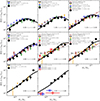 |
Fig. 8. IRX-M* relationship for the 0.5 < z ≤ 5.0 sample of this work. The black circles with error bars show IRX values median-stacked in bins of M* (Table A.3; same as color points in Figure 6). The black curves show corresponding best-fit functional forms summarized in Table 2 (same as color curves in Figure 6). For comparison, recent literature data of Whitaker et al. (2014), Heinis et al. (2014), Pannella et al. (2015), McLure et al. (2018), Koprowski et al. (2018), Álvarez-Márquez et al. (2019), Bouwens et al. (2020) and Fudamoto et al. (2020a) are also plotted, the discussion of which is presented in Section 4.5. |
The IRX-M* data found in Álvarez-Márquez et al. (2019) follows a significantly flatter relationship. As the authors explain in Álvarez-Márquez et al. (2019), the inconsistencies at low stellar masses are most likely caused by the incompleteness of their LBGs sample in terms of M*. Assuming the dependence of the stellar mass on the IRAC 3.6 μm flux density, the mass completeness at log(M*/M⊙) < 10 is between 80% and 50%, with lower-IRX sources missed from the sample. The IRX-M* data and the corresponding functional form found in Bouwens et al. (2020) is in a very good agreement with our results, with some inconsistencies at high stellar masses. At the highest redshift bin we can see the reported IRX stacked values of Fudamoto et al. (2020a) lying significantly below our data, likely due to the selection effects. As explained in Fudamoto et al. (2020a), the UV-selected samples at z > 4 may be missing a significant population of UV-undetected, massive galaxies (e.g., Wang et al. 2019; Alcalde Pampliega et al. 2019). Because the parent ALPINE sample of Fudamoto et al. (2020a) is UV-selected (MUV < −20.2), it inherently excludes a fraction of highly dust-obscured galaxies from their stacks. This selection bias explains why the discrepancy with our stacked values becomes more pronounced at higher stellar masses, where such heavily dusty sources constitute a larger fraction of the population. Between redshifts 3.0 and 4.0 at the highest mass bins our analysis produced somewhat elevated values of the IRX. We attribute these discrepancies to the fact that we were not able to remove all the starbursts from our sample. As explained in Section 3.1, starbursts were identified using the available ALMA data, which is not only incomplete in the COSMOS field, but is also biased against detecting sources with low dust masses and high dust temperatures. Since starbursts are known to exhibit very high dust content (e.g., Koprowski et al. 2018), their presence in the high-mass sample is expected to boost the resulting IRX values.
5. Summary
In this work, we investigate a K-band selected, mass-complete sample of 135,596 star-forming galaxies (spanning stellar masses of 9.5 ≤ log(M*/M⊙)≤11.5) from the UDS and COSMOS fields. The sample spans a combined ∼2 deg2 with extensive UV–near-IR coverage and FIR/sub-mm imaging from Herschel and JCMT. We established the quantitative dependence of IRX on UV slope, stellar mass, and redshift out to z ∼ 5 to provide functional prescriptions suitable for the dust correction of high-redshift galaxy samples. We adopted the available photometric redshifts and stellar masses from McLeod et al. (2021) and removed quiescent systems and ALMA-identified starbursts where possible. IR luminosities were obtained via inverse-variance stacking at 850 μm adopting Casey (2012) SEDs and a redshift-dependent dust temperature relation from Koprowski et al. (2024). UV slopes were derived from SED fits in the rest-frame 125–250 nm range, and the IRX was computed as the median of individual IRX values. The main results and key quantities can be summarized as follows:
-
(i)
The stacking in the UV slope bins reveals that at β ≳ −1.0, the IRX-β relation is consistent with a Calzetti-like attenuation law, yielding a best-fit dust-reddening slope of dA1600/dβ = 1.97, a bolometric correction BC(1600) = 1.51 ± 0.11, and an intrinsic UV slope of βint = −2.30 ± 0.10. At bluer UV slopes, however, the stacked values of the IRX increase with redshift. We find this systematic trend to be a direct consequence of the different mass-completeness limits imposed in each redshift bin, with higher z data effectively probing higher-mass galaxies at a given β.
-
(ii)
Stacking in stellar-mass bins between 2.0 < z ≤ 5.0, we find the IRX to systematically increase, at a given β, with mass relative to the nominal Calzetti-like IRX-β relation. This behavior demonstrates that dust-rich, massive systems are characterized by flatter (grayer) attenuation curves, likely driven by the combined effects of radiative transfer processes and increasingly disturbed dust-star relative morphologies. We explicitly quantified this through the effective slope of the reddening law, finding it follows a tight quadratic dependence on stellar mass: dA1600/dβ = ( − 0.30 ± 0.07)ℳ2 + (7.06 ± 1.40)ℳ − (38.8 ± 7.5), where ℳ = log(M*/M⊙), making IRX a bivariate function of β and M*.
-
(iii)
Expressing IRX directly as a function of M* yields a monotonic rise with mass out to z = 5.0. However, at z ≲ 2 − 3, a clear high-mass turnover is detected. This turnover indicates a rapid reduction in dust-obscured star formation (LIR, tracing young stars ≲10 Myr) relative to unobscured star formation (LUV, tracing older populations up to ∼100 Myr), most likely driven by supersonic shocks halting cold-gas accretion and starving massive galaxies of the fuel needed for dust growth. Accounting for a sSFR-dependent dust temperature would push our high-mass, low-redshift stacked IRX values lower, making the IRX-M* turnover even more pronounced. While our derived β–M* track tightly constrains the median behavior of this relation, individual galaxies exhibit a substantial intrinsic physical scatter around this median, widening from σβ,intr ≈ 0.3 at log(M*/M⊙) = 9.5 to σβ,intr ≈ 0.7 at log(M*/M⊙) = 11.5.
The results of this work are in broad agreement with previous stacking-based measurements (e.g., McLure et al. 2018; Álvarez-Márquez et al. 2019; Bouwens et al. 2020), while providing a comprehensive framework that resolves many literature inconsistencies. Much of the discrepancy in recently published relations can be largely resolved by incorporating the stellar-mass dependence of the reddening law and a careful SED-based estimation of β. Some of the remaining differences can be attributed to the dust emission curve modeling, where adopting a fixed dust temperature (e.g., Td = 30 K) ends up shifting our low-redshift stacked IRX values higher by ∼0.3 dex, as well as the selection effects, with purely UV-selected samples missing a substantial fraction of dust-obscured galaxies at high stellar masses. These effects result in significantly lower reported IRX values.
Data availability
Machine-readable versions of Table 1 and the Appendix tables are publicly available on Zenodo at https://doi.org/10.5281/zenodo.20392672.
Acknowledgments
This research was funded in whole or in part by the National Science Center, Poland (grant no. 2020/39/D/ST9/03078 and 2023/49/B/ST9/00066). For the purpose of Open Access, the author has applied a CC-BY public copyright license to any Author Accepted Manuscript (AAM) version arising from this submission. JSD, DJM acknowledge the support of the Royal Society through the award of a Royal Society University Research Professorship to JSD. KL acknowledges the support of the National Science Centre, Poland, through the PRELUDIUM grant UMO-2023/49/N/ST9/00746. This paper used data from project MJLSC02 on the James Clerk Maxwell Telescope, which is operated by the East Asian Observatory on behalf of The National Astronomical Observatory of Japan, Academia Sinica Institute of Astronomy and Astrophysics, the Korea Astronomy and Space Science Institute, the National Astronomical Observatories of China and the Chinese Academy of Sciences (Grant No. XDB09000000), with additional funding support from the Science and Technology Facilities Council of the United Kingdom and participating universities in the United Kingdom and Canada. This work is based in part on data products from observations made with ESO Telescopes at the La Silla Paranal Observatory under ESO program ID 179.A-2005 and ID 179.A-2006 and on data products produced by CALET and the Cambridge Astronomy Survey Unit on behalf of the UltraVISTA and VIDEO consortia. This work is based in part on data obtained as part of the UKIRT Infrared Deep Sky Survey. UKIRT is owned by the University of Hawaii (UH) and operated by the UH Institute for Astronomy; operations are enabled through the cooperation of the East Asian Observatory. When (some of) the data reported here were acquired, UKIRT was supported by NASA and operated under an agreement among the University of Hawaii, the University of Arizona, and Lockheed Martin Advanced Technology Center; operations were enabled through the cooperation of the East Asian Observatory. When (some of) the data reported here were acquired, UKIRT was operated by the Joint Astronomy Centre on behalf of the Science and Technology Facilities Council of the U.K. This work is also based in part on observations made with the Spitzer Space Telescope, which is operated by the Jet Propulsion Laboratory, California Institute of Technology under NASA contract 1407. This work is based in part on observations obtained with MegaPrime/MegaCam, a joint project of CFHT and CEA/IRFU, at the Canada-France-Hawaii Telescope (CFHT) which is operated by the National Research Council (NRC) of Canada, the Institut National des Science de l’Univers of the Centre National de la Recherche Scientifique (CNRS) of France, and the University of Hawaii.
References
- Alcalde Pampliega, B., Pérez-González, P. G., Barro, G., et al. 2019, ApJ, 876, 135 [NASA ADS] [CrossRef] [Google Scholar]
- Álvarez-Márquez, J., Burgarella, D., Buat, V., Ilbert, O., & Pérez-González, P. G. 2019, A&A, 630, A153 [NASA ADS] [CrossRef] [EDP Sciences] [Google Scholar]
- Ashby, M. L. N., Willner, S. P., Fazio, G. G., et al. 2013, ApJ, 769, 80 [Google Scholar]
- Ashby, M. L. N., Willner, S. P., Fazio, G. G., et al. 2015, ApJS, 218, 33 [NASA ADS] [CrossRef] [Google Scholar]
- Boquien, M., Burgarella, D., Roehlly, Y., et al. 2019, A&A, 622, A103 [NASA ADS] [CrossRef] [EDP Sciences] [Google Scholar]
- Bouwens, R. J., Aravena, M., Decarli, R., et al. 2016, ApJ, 833, 72 [NASA ADS] [CrossRef] [Google Scholar]
- Bouwens, R., González-López, J., Aravena, M., et al. 2020, ApJ, 902, 112 [NASA ADS] [CrossRef] [Google Scholar]
- Bruzual, G., & Charlot, S. 2003, MNRAS, 344, 1000 [NASA ADS] [CrossRef] [Google Scholar]
- Calzetti, D., Kinney, A. L., & Storchi-Bergmann, T. 1994, ApJ, 429, 582 [Google Scholar]
- Calzetti, D., Armus, L., Bohlin, R. C., et al. 2000, ApJ, 533, 682 [NASA ADS] [CrossRef] [Google Scholar]
- Calzetti, D., Wu, S.-Y., Hong, S., et al. 2010, ApJ, 714, 1256 [Google Scholar]
- Capak, P. L., Carilli, C., Jones, G., et al. 2015, Nature, 522, 455 [NASA ADS] [CrossRef] [Google Scholar]
- Casey, C. M. 2012, MNRAS, 425, 3094 [Google Scholar]
- Chabrier, G. 2003, PASP, 115, 763 [Google Scholar]
- Cullen, F., McLure, R. J., Khochfar, S., et al. 2018, MNRAS, 476, 3218 [Google Scholar]
- Daddi, E., Delvecchio, I., Dimauro, P., et al. 2022, A&A, 661, L7 [NASA ADS] [CrossRef] [EDP Sciences] [Google Scholar]
- Drew, P. M., & Casey, C. M. 2022, ApJ, 930, 142 [NASA ADS] [CrossRef] [Google Scholar]
- Dudzevičiūtė, U., Smail, I., Swinbank, A. M., et al. 2020, MNRAS, 494, 3828 [Google Scholar]
- Elbaz, D., Leiton, R., Nagar, N., et al. 2018, A&A, 616, A110 [NASA ADS] [CrossRef] [EDP Sciences] [Google Scholar]
- Fisher, R., Bowler, R. A. A., Stefanon, M., et al. 2025, MNRAS, 539, 109 [Google Scholar]
- Fudamoto, Y., Oesch, P. A., Faisst, A., et al. 2020a, A&A, 643, A4 [NASA ADS] [CrossRef] [EDP Sciences] [Google Scholar]
- Fudamoto, Y., Oesch, P. A., Magnelli, B., et al. 2020b, MNRAS, 491, 4724 [Google Scholar]
- Furusawa, H., Kosugi, G., Akiyama, M., et al. 2008, ApJS, 176, 1 [NASA ADS] [CrossRef] [Google Scholar]
- Geach, J. E., Dunlop, J. S., Halpern, M., et al. 2017, MNRAS, 465, 1789 [Google Scholar]
- Gebek, A., Diemer, B., Martorano, M., et al. 2025, A&A, 695, A90 [NASA ADS] [CrossRef] [EDP Sciences] [Google Scholar]
- Griffin, M. J., Abergel, A., Abreu, A., et al. 2010, A&A, 518, L3 [EDP Sciences] [Google Scholar]
- Gwyn, S. D. J. 2012, AJ, 143, 38 [Google Scholar]
- Heinis, S., Buat, V., Béthermin, M., et al. 2013, MNRAS, 429, 1113 [Google Scholar]
- Heinis, S., Buat, V., Béthermin, M., et al. 2014, MNRAS, 437, 1268 [Google Scholar]
- Ilbert, O., McCracken, H. J., Le Fèvre, O., et al. 2013, A&A, 556, A55 [NASA ADS] [CrossRef] [EDP Sciences] [Google Scholar]
- Ismail, D., Beelen, A., Buat, V., et al. 2023, A&A, 678, A27 [Google Scholar]
- Jarvis, M. J., Bonfield, D. G., Bruce, V. A., et al. 2013, MNRAS, 428, 1281 [Google Scholar]
- Kennicutt, R. C., & Evans, N. J. 2012, ARA&A, 50, 531 [NASA ADS] [CrossRef] [Google Scholar]
- Koprowski, M. P., Coppin, K. E. K., Geach, J. E., et al. 2018, MNRAS, 479, 4355 [NASA ADS] [CrossRef] [Google Scholar]
- Koprowski, M. P., Wijesekera, J. V., Dunlop, J. S., et al. 2024, A&A, 691, A164 [NASA ADS] [CrossRef] [EDP Sciences] [Google Scholar]
- Kriek, M., & Conroy, C. 2013, ApJ, 775, L16 [NASA ADS] [CrossRef] [Google Scholar]
- Lawrence, A., Warren, S. J., Almaini, O., et al. 2007, MNRAS, 379, 1599 [Google Scholar]
- Leslie, S. K., Schinnerer, E., Liu, D., et al. 2020, ApJ, 899, 58 [Google Scholar]
- Liang, L., Feldmann, R., Kereš, D., et al. 2019, MNRAS, 489, 1397 [NASA ADS] [CrossRef] [Google Scholar]
- Lisiecki, K., Donevski, D., Man, A. W. S., et al. 2025, arXiv e-prints [arXiv:2509.10117] [Google Scholar]
- Liu, D., Lang, P., Magnelli, B., et al. 2019, ApJS, 244, 40 [Google Scholar]
- Lo Faro, B., Buat, V., Roehlly, Y., et al. 2017, MNRAS, 472, 1372 [NASA ADS] [CrossRef] [Google Scholar]
- Lutz, D., Poglitsch, A., Altieri, B., et al. 2011, A&A, 532, A90 [NASA ADS] [CrossRef] [EDP Sciences] [Google Scholar]
- Madau, P. 1995, ApJ, 441, 18 [NASA ADS] [CrossRef] [Google Scholar]
- Madau, P., & Dickinson, M. 2014, ARA&A, 52, 415 [Google Scholar]
- Magnelli, B., Lutz, D., Saintonge, A., et al. 2014, A&A, 561, A86 [NASA ADS] [CrossRef] [EDP Sciences] [Google Scholar]
- McCracken, H. J., Milvang-Jensen, B., Dunlop, J., et al. 2012, A&A, 544, A156 [NASA ADS] [CrossRef] [EDP Sciences] [Google Scholar]
- McLeod, D. J., McLure, R. J., Dunlop, J. S., et al. 2021, MNRAS, 503, 4413 [NASA ADS] [CrossRef] [Google Scholar]
- McLure, R. J., Dunlop, J. S., Cullen, F., et al. 2018, MNRAS, 476, 3991 [Google Scholar]
- Mehta, V., Scarlata, C., Capak, P., et al. 2018, ApJS, 235, 36 [NASA ADS] [CrossRef] [Google Scholar]
- Meiksin, A. 2006, MNRAS, 365, 807 [Google Scholar]
- Mérida, R. M., Pérez-González, P. G., Sánchez-Blázquez, P., et al. 2023, ApJ, 950, 125 [CrossRef] [Google Scholar]
- Meurer, G. R., Heckman, T. M., & Calzetti, D. 1999, ApJ, 521, 64 [Google Scholar]
- Morales, A. M., Finkelstein, S. L., Leung, G. C. K., et al. 2024, ApJ, 964, L24 [NASA ADS] [CrossRef] [Google Scholar]
- Narayanan, D., Conroy, C., Davé, R., Johnson, B. D., & Popping, G. 2018, ApJ, 869, 70 [Google Scholar]
- Oliver, S. J., Bock, J., Altieri, B., et al. 2012, MNRAS, 424, 1614 [NASA ADS] [CrossRef] [Google Scholar]
- Pannella, M., Elbaz, D., Daddi, E., et al. 2015, ApJ, 807, 141 [Google Scholar]
- Pilbratt, G. L., Riedinger, J. R., Passvogel, T., et al. 2010, A&A, 518, L1 [NASA ADS] [CrossRef] [EDP Sciences] [Google Scholar]
- Poglitsch, A., Waelkens, C., Geis, N., et al. 2010, A&A, 518, L2 [NASA ADS] [CrossRef] [EDP Sciences] [Google Scholar]
- Popesso, P., Concas, A., Cresci, G., et al. 2023, MNRAS, 519, 1526 [Google Scholar]
- Reddy, N. A., Erb, D. K., Pettini, M., Steidel, C. C., & Shapley, A. E. 2010, ApJ, 712, 1070 [NASA ADS] [CrossRef] [Google Scholar]
- Reddy, N., Dickinson, M., Elbaz, D., et al. 2012, ApJ, 744, 154 [NASA ADS] [CrossRef] [Google Scholar]
- Reddy, N. A., Oesch, P. A., Bouwens, R. J., et al. 2018, ApJ, 853, 56 [NASA ADS] [CrossRef] [Google Scholar]
- Rogers, A. B., McLure, R. J., & Dunlop, J. S. 2013, MNRAS, 429, 2456 [Google Scholar]
- Salim, S., & Narayanan, D. 2020, ARA&A, 58, 529 [NASA ADS] [CrossRef] [Google Scholar]
- Salmon, B., Papovich, C., Long, J., et al. 2016, ApJ, 827, 20 [NASA ADS] [CrossRef] [Google Scholar]
- Shivaei, I., Naidu, R. P., Rodríguez Montero, F., et al. 2026, A&A, in press, https://doi.org/10.1051/0004-6361/202557064 [Google Scholar]
- Stach, S. M., Dudzevičiūtė, U., Smail, I., et al. 2019, MNRAS, 487, 4648 [Google Scholar]
- Tomczak, A. R., Quadri, R. F., Tran, K.-V. H., et al. 2016, ApJ, 817, 118 [Google Scholar]
- van der Wel, A., Martorano, M., Marchesini, D., et al. 2025, A&A, 701, A30 [NASA ADS] [CrossRef] [EDP Sciences] [Google Scholar]
- Viero, M. P., Sun, G., Chung, D. T., Moncelsi, L., & Condon, S. S. 2022, MNRAS, 516, L30 [NASA ADS] [CrossRef] [Google Scholar]
- Wang, L., Pearson, W. J., Cowley, W., et al. 2019, A&A, 624, A98 [NASA ADS] [CrossRef] [EDP Sciences] [Google Scholar]
- Whitaker, K. E., Franx, M., Leja, J., et al. 2014, ApJ, 795, 104 [NASA ADS] [CrossRef] [Google Scholar]
Appendix A: Additional tables
IRX values median-stacked in bins of β and redshift.
IRX values median-stacked in bins of β.
IRX-M* stacked values.
All Tables
All Figures
|
Fig. 1. IRX-β relationship for 2.0 < z ≤ 5.0 sample studied in this work. The color points with error bars show the stacked values of the IRX in bins of β, summarized in Table A.1. The black solid line represents the best-fit functional form (Equation 9), with dA1600/dβ = 1.97 being consistent with the attenuation curve of Calzetti et al. (2000). The scatter at β ≲ −1 is caused by different stellar mass completeness limits imposed at each redshift bin (see Section 4.1 for details). For reference, the SMC curve is plotted in dashed line. |
| In the text | |
|
Fig. 2. Relationship between the UV slope and the stellar mass for the sample presented in Figure 1. Green background image shows a 2D histogram of the β–M* distribution, with 1, 10, 100 and 1000 sources contours displayed with black curves. It can be seen that due to different mass-completeness limits imposed at each redshift bin (Table A.1), the median stellar masses at bluest β bins increase with redshift, which in turn drives the scatter in Figure 1 (see Section 4.1 for details). |
| In the text | |
|
Fig. 3. IRX-β relationship in bins of stellar mass. The black circles show the stacked data (Table 1), with a clear correlation between the stellar mass and the slope of the reddening law, dA1600/dβ. Adopting Equation (9), with dA1600/dβ set as free parameter, best-fit values for the reddening slope were found (last column in Table 1), with the corresponding correlation with the stellar mass derived in Section 4.2 and plotted in Figure 4. For reference, this work’s best-fit relationship (consistent with the Calzetti curve), together with the SMC curve are plotted in solid and dashed lines, respectively. |
| In the text | |
|
Fig. 4. Relationship between the dust reddening slope, dA1600/dβ, and the stellar mass for the sample plotted in Figure 3, where a clear correlation can be seen, with more massive systems being characterized by flatter attenuation curves. The functional form of the relation is derived and discussed in Section 4.2 and summarized in Equation (9). |
| In the text | |
|
Fig. 5. IRX-β relationship derived for the 2.0 < z ≤ 5.0 sample of this work (gray circles; Table A.2). Top panel. Our median data lying slightly below the best-fit curve at blue UV slopes is driven by variations in the corresponding median stellar masses. We compare our data with the recent literature results of Heinis et al. (2013), Reddy et al. (2018), McLure et al. (2018), Koprowski et al. (2018), Álvarez-Márquez et al. (2019), Fudamoto et al. (2020b) and Bouwens et al. (2020). For reference, this work’s best-fit relationship and the SMC-like curve are plotted in solid and dashed lines, respectively. Bottom panel. To investigate the literature scatter, we highlight how varying data treatment methodologies alters our results (gray circles). Adopting a dust temperature of Td = 40 K with a restricted stellar mass of log(M*/M⊙)∼10.5 (green squares), or deriving UV slopes via photometric power-law fitting instead of best-fit SEDs (red crosses), radically changes the shape and normalization of the relation, mirroring the scatter seen in the top panel. See Section 4.3 for details. |
| In the text | |
|
Fig. 6. IRX values median-stacked in bins of M* and redshift (color points with error bars; Table A.3). The black line shows the best-fit functional form for the 2.0 < z ≤ 5.0 sample of Figure 3, while the color solid lines depict the functional forms found at the individual redshift bins, as explained in detail in Section 4.4. |
| In the text | |
|
Fig. 7. The relationship between the observed UV slope and stellar mass for the 2.0 < z ≤ 5.0 sample of this work. Green background image represents a 2D histogram of the β–M* distribution, with 1, 10, 100 and 1000 sources contours displayed with thin black curves. Top panel. Black circles with error bars show median values of β in bins of M* (Table 1), with the thick black solid curve depicting the best-fit functional form of Equation (12). For comparison, the relationships found in McLure et al. (2018), Álvarez-Márquez et al. (2019) and Bouwens et al. (2020) are shown. Bottom panel. Black curve as in the top panel with the color curves determined for individual redshift bins, following the procedure explained in Section 4.4. |
| In the text | |
|
Fig. 8. IRX-M* relationship for the 0.5 < z ≤ 5.0 sample of this work. The black circles with error bars show IRX values median-stacked in bins of M* (Table A.3; same as color points in Figure 6). The black curves show corresponding best-fit functional forms summarized in Table 2 (same as color curves in Figure 6). For comparison, recent literature data of Whitaker et al. (2014), Heinis et al. (2014), Pannella et al. (2015), McLure et al. (2018), Koprowski et al. (2018), Álvarez-Márquez et al. (2019), Bouwens et al. (2020) and Fudamoto et al. (2020a) are also plotted, the discussion of which is presented in Section 4.5. |
| In the text | |
Current usage metrics show cumulative count of Article Views (full-text article views including HTML views, PDF and ePub downloads, according to the available data) and Abstracts Views on Vision4Press platform.
Data correspond to usage on the plateform after 2015. The current usage metrics is available 48-96 hours after online publication and is updated daily on week days.
Initial download of the metrics may take a while.