


| Issue |
A&A
Volume 711, July 2026
|
|
|---|---|---|
| Article Number | A49 | |
| Number of page(s) | 15 | |
| Section | Galactic structure, stellar clusters and populations | |
| DOI | https://doi.org/10.1051/0004-6361/202659254 | |
| Published online | 02 July 2026 | |
The intrinsic dispersion of elemental abundance ratios in nearby metal-poor halo stars★
1
Department of Physics and Astronomy, Aarhus University,
Ny Munkegade 120,
8000
Aarhus C,
Denmark
2
Theoretical Astrophysics, Department of Physics and Astronomy, Uppsala University,
Box 516,
751 20
Uppsala,
Sweden
★★ Corresponding author: This email address is being protected from spambots. You need JavaScript enabled to view it.
Received:
31
January
2026
Accepted:
27
April
2026
Abstract
Context. Elemental abundance ratios in halo stars provide information on nucleosynthesis, chemical evolution, and accretion of dwarf galaxies at early times in the Milky Way because these ratios depend on the initial mass function (IMF) of core-collapse supernovae (CC SNe) and on the role of Type Ia SNe in making the elements.
Aims. By determining very precise stellar parameters and abundances for a sample of intermediate-metallicity halo stars, we aim to estimate the intrinsic dispersion of various abundance ratios.
Methods. We determined differential abundances of C, O, Mg, Al, Ca, Sc, Ti, V, Cr, Mn, Fe, Co, Ni, Zn, Y, and Zr from high signal-to-noise VLT/UVES spectra for 25 turnoff stars with −2.4 < [Fe/H] < −1.3. Effective temperatures were obtained from profiles of the Hβ line and surface gravities from Gaia parallaxes. The spectral analysis was based on 1D model atmospheres assuming local thermodynamic equilibrium (LTE), but we applied 3D non-LTE corrections for several elements.
Results. The dispersion in linear fits to the [X/Fe]-[Fe/H] relations is around a factor of two smaller than that found in previous studies. After correction for measurement errors, the 1σ intrinsic dispersion of [X/Fe] at a given metallicity is 0.09 dex for Y and Zr, 0.05-0.07 dex for C, O, and Al, 0.03-0.05 dex for Mg, Ca, Sc, Ti, V, Mn, and Zn, and <0.03 dex for Cr, Co, and Ni. We find strong correlations between the residuals in the [X/Fe]-[Fe/H] fits for the α-capture elements (Mg, Al, Ca, Sc, and Ti) and between the residuals for Y and Zr.
Conclusions. Correlations between the residuals in the [X/Fe]-[Fe/H] fits and the effective temperature can be explained by differential atomic diffusion between elements, but its contribution to the scatter of [X/Fe] is of minor importance. Both stochastic effects in sampling the IMF of CC SNe and differences in the Type Ia to CC SNe enrichment ratio between star-forming regions are likely required to explain the intrinsic dispersion of [X/Fe].
Key words: stars: abundances / stars: atmospheres / supernovae: general / Galaxy: formation / Galaxy: halo
Based on data products from observations made with ESO Telescopes at the La Silla Paranal Observatory under programmes 67.D-0106 and 73.D-0024.
© The Authors 2026
 Open Access article, published by EDP Sciences, under the terms of the Creative Commons Attribution License (https://creativecommons.org/licenses/by/4.0), which permits unrestricted use, distribution, and reproduction in any medium, provided the original work is properly cited.
This article is published in open access under the Subscribe to Open model. This email address is being protected from spambots. You need JavaScript enabled to view it. to support open access publication.
1 Introduction
Trends in abundance ratios as a function of metallicity ([Fe/H]1) provide important constraints on Galactic chemical evolution (GCE) models, but the scatter at a given metallicity is also of great interest, as shown in high-precision studies of the Galactic disc (Edvardsson et al. 1993; Fuhrmann 1998; Gratton et al. 2000; Adibekyan et al. 2012) and the Galactic halo (Cayrel et al. 2004; Cohen et al. 2004; Arnone et al. 2005). It came as a surprise that these studies found that very metal-poor halo stars (−4.0 < [Fe/H] < −2.5) showed a 1σ dispersion of only ∼0.1 dex in the abundances of α-capture elements relative to iron ([α/Fe]). In comparison, GCE models, in which only a few core-collapse supernovae (CC SNe) contributed to the enrichment of interstellar clouds, predicted dispersions of the order of 0.4 dex in [α/Fe] (Audouze & Silk 1995; Argast et al. 2000, 2002). This discrepancy led to new stochastic GCE models (e.g. Karlsson 2005; Karlsson & Gustafsson 2005; Cescutti 2008) and further studies of the dispersion of abundance ratios in very metal-poor stars, of which Li et al. (2022) is the most precise and extensive. Based on high-resolution spectra of 385 stars covering the metallicity range –4.3 < [Fe/H] < –1.7, they find dispersions in [Mg/Fe], [Ca/Fe], and [Ti/Fe] ≲ 0.08 dex, whereas the dispersion in the abundance of neutron-capture elements relative to iron is about 0.15 dex.
In the more metal-rich part of the Galactic halo, that is, for stars with metallicities [Fe/H] > –1.3, the dispersion in [X/Fe] for many elements, including Na, Mg, Al, Ca, Ti, and Ni, is larger than in very metal-poor stars. A high-precision study of abundances of 94 dwarf stars by Nissen & Schuster (2010, 2011, hereafter NS10, NS11), later confirmed by Hawkins et al. (2015) and Hayes et al. (2018) using a larger sample of K giants with APOGEE spectra, shows that the more metal-rich part of the halo splits into two populations: high-α stars born in situ in the Milky Way and low-α stars accreted from dwarf galaxies, of which the so-called Gaia-Sausage-Enceladus (GSE) galaxy is the most important (Helmi 2020). According to NS11, the mean separation of [Mg/Fe] at [Fe/H] = –0.9 between high-a and low-α stars is 0.22 dex and the measured dispersion for the accreted population, σ[Mg/Fe] = 0.055 dex, is significantly higher than that for in situ stars, σ[Mg/Fe] = 0.029 dex. This can be explained by variations in the Type Ia SNe contribution to iron among dwarf galaxies and by the formation of high-α stars in regions where only CC SNe contributed to the chemical evolution. Furthermore, there are significant differences in [X/Fe] between in situ and accreted stars for other elements, for example, Na, Ca, Ti, and Ni, with the dispersion for accreted stars always being the highest (e.g. Figs. 4 and 8 of NS11).
The dispersions reported in NS11 were challenged by Belokurov & Kravtsov (2022), who used [Al/Fe] abundance ratios from APOGEE and kinematics from Gaia data to separate a large sample of red giant stars into in situ and accreted populations. According to their Fig. 7, the dispersions in [X/Fe] for the two populations are about the same at [Fe/H] = –1.0 and about a factor of two higher than the estimated measurement error, σcbs – 0.02 dex. There is, however, a sharp increase in the dispersion of [X/Fe] for the in situ stars towards lower metallicities, i.e. [Fe/H] = –1.4, especially for N, Al, Mg, and Si, whereas the dispersion is approximately constant for the accreted stars. This is interpreted as arising from a period of chaotic pre-disc evolution of the Galaxy, dubbed Aurora, with bursty star formation.
It is also interesting to compare the measured dispersions in NS11 with those determined by Griffith et al. (2023) in a high-precision abundance study of a sample of 86 subgiant stars with –2.0 < [Fe/H] < –1.0. After correcting for measurement errors, Griffith et al. derived intrinsic dispersions in linear fits of [X/Fe] as a function of [Fe/H] and [α/Fe]. For the α-capture elements, Mg, Si, Ca, and Ti, they find σintrin ≃ 0.05 dex, i.e. about a factor of two higher than the measured dispersions in NS11 for the high-α population. They ascribe this intrinsic scatter to stochastic sampling of the CCSNe progenitor mass distribution and estimate that ejecta from –50 CC SNe are mixed over gas masses of ∼6 × 10⁴ M⊙.
For intermediate-metallicity (–2.5 < [Fe/H] < –1.5) halo stars, high-precision abundance studies aimed at determining intrinsic dispersions are sparse. The most precise study is that of Reggiani et al. (2017), who determined differential abundance ratios for a sample of 23 nearby stars situated in the turnoff region of the HR diagram. The standard deviation in linear fits of [X/Fe] versus [Fe/H] is close to 0.06 dex for Mg, Si, Ca, and Ti, which is of the same order of size as the estimated measurement error, leaving very little room for intrinsic dispersion, in contrast to the results of Griffith et al. (2023).
These studies typically employ 1D hydrostatic model atmospheres and assume local thermodynamic equilibrium (LTE). The wider the span in stellar parameters, particularly effective temperature (Teff), surface gravity (log g), and metallicity, the greater the potential for errors due to the 1D LTE assumption to affect the measured dispersion (e.g. Nissen & Gustafsson 2018; Amarsi et al. 2019c). The exact span in stellar parameters at which the 3D non-LTE effects must be accounted for depends on the line and stellar parameters in question. For example, the resonant Mg I 4571.1 Å intercombination line is a severe case: changes of around 200 K in Teff, 0.25 dex in log g, or 0.5 dex in [Fe/H], produce differential 3D non-LTE versus 1D LTE abundance corrections of around 0.05 dex relative to HD 110621, according to the models used in the present study. The subordinate Mg I 4703.0 Å permitted line is less sensitive and requires changes at least twice as large to produce similar differential corrections. Griffith et al. (2023) found that 1D non-LTE effects do not significantly affect the scatter in their sample; however, this has yet to be confirmed with independent and more recent model atoms, as well as with a consistent 3D non-LTE approach.
In this paper, we aim to determine very precise abundance ratios for a sample of 25 dwarf stars with –2.4 < [Fe/H] < –1.3 and VLT/UVES spectra with signal-to-noise ratios (S/N) ≳ 200. By determining Teff with a precision of ±30 K, log g with a precision of ±0.03 dex, and by considering 3D non-LTE effects in the abundance analysis, errors of determining [X/Fe] approach a level of ±0.02 dex, making it possible to improve estimates of intrinsic scatter and thus learn more about the nucleosynthesis of elements in the early Galaxy.
2 Sample selection and stellar spectra
We selected stars from a sample of 40 dwarf and subgiant stars for which we previously determined sulphur and zinc abundances (Nissen et al. 2004, 2007), as well as carbon and oxygen abundances (Akerman et al. 2004; Fabbian et al. 2009; Amarsi et al. 2019b). Only stars in the turnoff region (6000 K ≲ Teff ≲ 6400 K and 3.8 < log g < 4.4) were included to minimise possible effects of errors in effective temperature and surface gravity as well as parameter-dependent errors in the 1D LTE spectroscopic models. Furthermore, we excluded stars with [Fe/H] < –2.4 because the spectral lines applied are too weak for such stars to be used for precise abundance determinations. We also omitted a few stars with [Fe/H] > –1.3, as they belong to the more metal-rich part of the halo, where the splitting into high-a and low-α stars is already well established. These selection criteria resulted in a sample of 25 stars.
The papers cited above describe the UVES spectral reduction. The spectra include a blue region (3750-5000 Å) previously used to determine Fe and Zn abundances and a near-IR region (6700-10500 Å) used to derive C, O, and S abundances. The spectral resolution is λ/∆λ = 60000 and the S/N per spectral resolution element is 200-300. In this study, we used only the blue part, taking advantage of the fact that this region contains lines suitable for precise determinations of the abundances of Mg, Al, Ca, Sc, Ti, V, Cr, Mn, Fe, Co, Ni, Zn, Y, and Zr (see Table A.1). We measured equivalent widths (EWs) of these lines with the IRAF splot task, using the same nearby line-free spectral windows to set the continuum for all stars. Most of the lines have EW< 80 mÅ and can be well fitted with a Gaussian profile. Exceptions are the Mg I 4703.0 and Al I 3961.5 Å lines, which we fitted with Voigt profiles.
The typical error of the EWs measured in the blue UVES spectra was estimated by Nissen et al. (2004, see their Fig. 3) to be ±0.6 mÅ, based on a comparison of EWs measured for six stars that have two spectra observed on different nights. As an example of the quality of the spectra, Fig. 1 shows a few lines for two stars with similar atmospheric parameters and metallicities. The small differences between the two stars in the EWs of the lines are mainly due to differences in log g and [Fe/H]; they have almost identical [Ca/Fe] and [Ti/Fe] ratios.
3 Stellar parameters
3.1 Effective temperature
We adopted the effective temperatures of the stars from Amarsi et al. (2019b), who determined Teff by fitting 3D non-LTE profiles of the Hβ line (Amarsi et al. 2018b) to the profiles in our spectra. The surface gravities in the present study are slightly different from those in Amarsi et al. (2019b) because we updated the Gaia parallaxes from DR2 to DR3; the metallicities also differ slightly. However, since the Hβ profiles are only weakly sensitive to log g and [Fe/H] (with effective temperature variations of about 20 K for changes of 0.3 dex in log g or [Fe/H] in metal-poor dwarfs; see Table 3 of Amarsi et al. 2018b), we did not correct for these small changes.
As discussed in Nissen et al. (2007), spectra obtained on different nights for a given star suggest that Teff derived from Hβ profiles can be determined with an internal 1σ precision of 20 K. To obtain an external estimate of the error, we compared the Teff values in Amarsi et al. (2019b) with those determined by Giribaldi et al. (2021) from fitting observed Hα profiles to the grid of 3D non-LTE line profiles in Amarsi et al. (2018b). Figure 2 shows the comparison for 15 stars in common. There is a systematic difference of about 100 K demonstrating the well-known difficulty in establishing an accurate absolute Teff scale. Amarsi et al. (2018b) show that the two features have different dominant uncertainties: Hα is particularly sensitive to departures from LTE, which tend to raise the inferred Teff, whereas Hß shows a high sensitivity to the atmospheric structure (as indicated by a higher sensitivity to mixing-length parameters in 1D models). From a modelling perspective, it is unclear which should be preferred.
Nevertheless, the standard deviation around the fitted line in Fig. 2 is only 44 K. This corresponds to a precision of about 30 K for each of the two ways of determining Teff, assuming that the two Teff measurements are independent and have similar random uncertainties. This is close to the median uncertainty of 34 K in Table 2 of Giribaldi et al. (2021). This level of precision matters when discussing differential abundance ratios for our sample of stars.
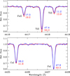 |
Fig. 1 Comparison of Ca, Ti, and Fe lines in spectra of two stars with similar atmospheric parameters and abundances. The spectrum of G59-27 (Teff = 6232K, log g = 4.22, [Fe/H] = −1.90, [Ca/Fe] = 0.42, and [Ti/Fe] = 0.33) is shown in blue, and that of CD–3018140 (Teff = 6241K, log g = 4.15, [Fe/H] = −1.84, [Ca/Fe] = 0.42, and [Ti/Fe] = 0.34) in red. For each line the measured equivalent widths for the two stars are given in mÅ with an estimated uncertainty of ±0.6 mÅ. |
3.2 Surface gravity
We determined the surface gravity of a star from the relation
 (1)
(1)
where M is the mass and Mbol is the absolute bolometric magnitude. The Gaia DR3 parallax (Gaia Collaboration 2023) was used to derive the absolute visual MV magnitude from the V magnitude based on Strömgren photometry (Nissen et al. 2007, Table B.1). The interstellar absorption (AV) was estimated from the colour excess E(b - y) using the (b - y)0 - β relation of Schuster & Nissen (1989), adopting a spectroscopic Hβ index instead of the photometric one to improve precision (Nissen et al. 2007). The bolometric correction (BC) was derived from V - K with the K magnitude from Cutri et al. (2003) using the calibration by Casagrande et al. (2010), and the stellar mass was obtained by interpolating in the luminosity - log Teff diagram between the Yonsei -Yale evolutionary tracks (Yi et al. 2003), assuming [α/Fe] = 0.4.
In estimating the uncertainty of log g, we accounted for the parallax error, ±30 K for Teff, and errors of ±0.02 mag for V and AV (Nissen et al. 2007) and BC (Casagrande et al. 2010). These errors propagate to an error of ±0.05 M⊙ in the stellar mass determined from the evolutionary tracks in the luminosity - log Teff diagram. When adding the corresponding errors in log g in quadrature, we obtain errors in the surface gravity of around 0.03 dex. The high precision of the Gaia DR3 parallaxes, together with distances from the Sun of less than 300 pc for our sample, makes the parallax-induced error in log g smaller than the other error sources, in contrast to Amarsi et al. (2019b), who used DR2 parallaxes.
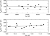 |
Fig. 2 Comparison of effective temperatures determined by Giribaldi et al. (2021) from Hα profiles and those of Amarsi et al. (2019b) from Hβ profiles. |
4 Elemental abundances
4.1 1D LTE analysis
Assuming LTE, we used the Uppsala EQWIDTH or BSYN programmes to calculate EWs as a function of element abundance for model atmospheres obtained by linear interpolation2 in the standard ([α/Fe] = 0.4) 1D MARCS grid (Gustafsson et al. 2008) matched to the Teff, log g, and [Fe/H] values of the stars. We then determined the abundance corresponding to a given line from the observed EW and obtained microturbulence (ξturb) values by requiring that Fe abundances derived from ∼60 Fe I lines have zero slope as a function of reduced equivalent width (EW/λ).
The analysis is differential with respect to a standard star, HD 110621, which has a spectrum with a particularly high S/N (∼400) and a metallicity [Fe/H] = –1.53. We first performed an abundance analysis of this star adopting the gf-values given in Table A.1. The resulting abundances are subject to systematic and statistical errors in the gf values, which are typically of order ±0.05 dex. For a given element, we then adopted the mean of the derived abundances for HD 110621 and altered the gf-values so that all lines of the element provide this mean abundance. These revised gf-values were used in the analysis of the other stars, which means that their differential abundances with respect to HD 110621 are not affected by errors in the gf-values. It also allows for the determination of differential values of ξturb with a precision of ±0.1 km s−1, as estimated from the error of the slope of the Fe abundance versus reduced EW.
Van der Waals broadening due to collisions with neutral hydrogen and helium atoms follows the Anstee-Barklem-O’Mara (ABO) calculations (see Barklem 2016) for lines marked ‘A’ in Table A.1. For lines marked ‘U’, we applied the Unsöld (1955) approximation with an enhancement factor of 1.5.
We accounted for hyperfine structure (hfs) broadening for the lines of Al, Sc, V, Mn, and Co by adopting data from the following sources: Al (Brown & Evenson 1999, VALD3), Sc (Lawler et al. 2019), V (Wood et al. 2014a), Mn (McWilliam et al. 1995), and Co (Lawler et al. 2015). Whereas the effect on the derived abundances of Al, Sc, V, and Mn is negligible due to a relatively small hfs splitting, the effect on the Co abundances derived from the 4121.3 Å Co I line is appreciable. The standard deviation of the linear fit to [Co/Fe] versus [Fe/H] decreases from 0.036 dex without hfs to 0.024 dex when hfs splitting is included. In addition, the slope of [Co/Fe] versus [Fe/H] is significantly affected.
We calculated the error in the abundance determination of an element X for a given star arising from the uncertainties in the EW measurements as  , where σX,line is the standard deviation in the line-to-line scatter of the abundance of X and NX is the number of lines4. As the S/N of the spectra and the number of lines applied for the various stars are much the same, we calculated an average error 〈σX〉. This average error was employed for the whole sample on a per-element basis. The corresponding average error of [X/Fe] is then
 (2)
(2)
To this we added in quadrature the uncertainties in [X/Fe] arising from Teff (±30 K), log g (±0.03 dex), and ξturb (±0.1 km s−1), which are similar for all stars because of their similarity in the parameters. In this way, we obtain a representative 1σ ‘observational’ error, σobs, for [X/Fe] which we used when calculating the intrinsic dispersion of linear fits of [X/Fe] as a function of [Fe/H] (see Sect. 5).
4.2 Corrections for 3D (non)-LTE effects
For some elements, we used 3D LTE or 3D non-LTE radiative transfer calculations to obtain corrections to the derived 1D LTE abundances. In the following, we describe these calculations and discuss the impact of the corrections on the abundances. For brevity, we use the following notation:
3N-1L = A (3D non-LTE) - A (1D LTE)
3L-1L = A (3D LTE) - A (1D LTE),
where A denotes the logarithmic abundance. We stress that in the [X/Fe]-[Fe/H] plots presented in subsequent sections, the abundance of the reference element Fe appearing in both [X/Fe] and [Fe/H] is based on 3D LTE abundances inferred from Fe II lines, regardless of the type of model used for the diagnostic element X. As the 3D corrections for Fe are not a strong function of stellar parameters and the non-LTE effects are negligible (Sect. 4.2.6), the trends would not be significantly affected if 1D LTE or 3D non-LTE Fe abundances were instead adopted in the ratio [X/Fe].
We based the 3D LTE and 3D non-LTE abundance corrections on the Stagger grid of 3D stellar atmosphere models by Magic et al. (2013) (see also Rodríguez Díaz et al. (2024) and Stein et al. (2024). For C, O, Mg, Ca, and Fe, we post-processed these models using the 3D non-LTE code Balder (Amarsi et al. 2018a), an offshoot of Multi3D (Botnen & Carlsson 1999; Leenaarts & Carlsson 2009). For the lines of ionised Ti, we instead calculated corrections using the 3D LTE code Scate (Hayek et al. 2011), with updates to the input data described in Amarsi et al. (2021). Historically, the accuracy of non-LTE modelling has been hampered by unrealistic treatments of inelastic collisions with neutral hydrogen; these limitations could potentially introduce additional scatter into the abundances (e.g. Caliskan et al. 2025). In the present study, all of the model atoms used for 3D non-LTE corrections employ modern descriptions for these processes that are based on asymptotic model approaches (e.g. Barklem et al. 2021) rather than the outdated Drawin approximation.
The 3D models naturally take into account line broadening caused by stellar granulation without additional free parameters, whereas in 1D, we accounted for the effect of the small-scale velocity field on the EWs with the microturbulence ‘nuisance’ parameter (e.g. Ludwig & Steffen 2016). The 3N - 1L and 3L-1L abundance corrections are a function of the microturbulence parameter adopted in the 1D LTE analysis. This ensures that the 3D abundances are independent of the choice of the 1D microturbulence parameter.
4.2.1 Carbon and oxygen
Carbon abundances were derived from up to seven C I lines in the 9000-9500 Å spectral range, and O abundances from the OI triplet at 7772-7775 Å by Nissen et al. (2002), Akerman et al. (2004), and Fabbian et al. (2009) using EWs measured in VLT/UVES spectra. Amarsi et al. (2019b) used the same data to derive C and O abundances for our sample, but we updated their results using the new stellar parameters.
We adopted 3N - 1L corrections from Amarsi et al. (2019c), which are based on model atoms described in Amarsi et al. (2018a) and Amarsi et al. (2019a). The provided routines were used to interpolate to the updated stellar parameters (Teff, log g, [Fe/H], ξturb, and A(C) or A(O)) used in this work. For carbon, the 3N - 1L corrections range from about –0.05 dex at [Fe/H] = –1.3 to –0.15 dex at [Fe/H] = –2.3, with a dispersion of 0.025 dex. The oxygen corrections have the opposite trend, ranging from about –0.13 dex to –0.07 dex over the same metallicity range, and a dispersion of only 0.017 dex for our sample. All three O I lines arise from the same multiplet; therefore, the 3D non-LTE effects for the O I lines have the same sign, are of similar magnitude, and show similar sensitivities to stellar parameters. This also applies to the CI lines, of which six belong to the same multiplet, while the seventh has an excitation energy close to that of the other six (see Table 1 of Amarsi et al. 2019a). Consequently, the line-to-line scatter is essentially unchanged after introducing the 3N-1L corrections, as are the standard deviations of the fits of [X/Fe] versus [Fe/H]. However, the slopes of the [X/Fe]-[Fe/H] relations are significantly affected due to the rather strong dependence of the 3N-1L corrections on [Fe/H].
 |
Fig. 3 Difference in Mg abundances derived from the 4703.0 and 4571.1 Å lines as a function of [Fe/H] normalised to zero for the standard star, HD 110621. |
4.2.2 Magnesium
We derived the Mg abundances from two Mg I lines: the 4571.1 Å line with a lower-level excitation potential χexc = 0.00 eV and the 4703.0 Å line with χexc = 4.34 eV. The first line is quite weak with the EWs ranging from ∼3 to ∼30 mÅ over the metallicity range of our stars, whereas the EW of the 4703.0 Å line ranges from ∼40 to ∼130 mÅ.
We based the 3N - 1L corrections on the calculations presented in Matsuno et al. (2024), which adopt the model atom described in Asplund et al. (2021). These data were interpolated onto the stellar parameters Teff, log g, ξturb, and A (Mg). The correction for the 4571.1 Å line varies strongly with [Fe/H], from approximately –0.05 dex at [Fe/H] = –1.3 to +0.15 dex at [Fe/H] = –2.3. The correction for the 4703.0 Å line is more constant, at a level of 0.10-0.15 dex depending on Teff and log g. Interestingly, applying the 3N-1L corrections improves the agreement between the Mg abundances derived from the two lines (Fig. 3). The trend in the difference in A (Mg) is flatter, and the dispersion is smaller in 3D non-LTE compared to 1D LTE; 〈σMg〉 calculated from the line-to-line scatter decreases from 0.026 dex in 1D LTE to 0.019 dex in 3D non-LTE. Despite this improvement in 〈σMg〉, the standard deviation of the fit to [Mg/Fe] versus [Fe/H] does not change significantly due to the 3N- 1L corrections. However, this does not imply that the 3N-1L corrections are unimportant. As discussed in Sect. 5, the corrections strengthen the correlation between the residuals in the [Mg/Fe]- [Fe/H] relation and those of the other α-capture elements.
4.2.3 Aluminium
The only lines in our spectra available for determining Al abundances are the resonance doublet at 3944.0 and 3961.5 Å. The 3944.0 Å line is distorted by Cr II and Ce II lines (Ernandes et al. 2025) and is not suitable for precise abundance determinations.
The 3961.5 Å line has a good profile but lies in the broad wings of the hydrogen Hε line at 3970.1 Å and the Ca II line at 3968.5 Å, which depress the flux at the wavelength of the Al I line by 510% for our stars. To account for this, we measured the EW of the Al I line relative to the flux in the wings of He and Ca II lines and calculated a corresponding EW from a synthetic spectrum that includes the contribution to the line absorption coefficient from the two broad lines. We calculated the He profile as in Barklem et al. (2002) and for the calculation of the Ca II line we adopted log gf = –0.18 from the NIST database (Kramida et al. 2024) and Ca abundances from the present work.
We computed 3N- 1L corrections specifically for this study using the model atom of Nordlander & Lind (2017). The calculations used 3D models with Teff of approximately 6000 and 6500 K, log g of 4.0 and 4.5, and [Fe/H] of –1, –2, and –3. For post-processing calculations, we varied [Al/Fe] between –0.8 dex and +0.4 dex in steps of 0.4 dex. We downsampled the 3D models horizontally by a factor of three (number of mesh points: 2402 → 802) and upsampled them vertically, and performed post-processing for five snapshots; this approach is sufficient for determining reliable abundance corrections based on EWs (Rodríguez Díaz et al. 2024). For the mean radiation field, we used 26 rays across the unit sphere, based on the eightpoint Lobatto quadrature between –1 ≤ μ ≤ 1 and the four-point trapezoidal quadrature between 0 ≤ φ ≤ 2π. For emergent disc-integrated flux, we used 41 rays across the unit hemisphere, based on the seven-point Lobatto quadrature between 0 ≤ μ ≤ 1 and the eight-point trapezoidal quadrature between 0 ≤ φ ≤ 2π. We also performed 1D LTE and 1D non-LTE calculations on ATMO model atmospheres (the 1D equivalent of the Stagger models; see Appendix A of Magic et al. 2013). These calculations were performed in an analogous way, but covering a wider and finer grid of [X/Fe] and also introducing a microturbulence parameter, ξturb = 0, 1, 1.5, and 2 km s−1.
The EW of the 3961.5 Å line ranges from about 60 mÅ to more than 150 mÅ over the metallicity range of our stars. At [Fe/H] = –2.3, the 3N-1L correction is as large as ∼0.6dex, decreasing to ∼0.4 dex at [Fe/H] = –1.3. At a given metallicity, variations in 3N- 1L of up to 0.1 dex occur depending on Teff and log g. The 3N - 1L corrections have little effect on the dispersion of the [Al/Fe]-[Fe/H] relation, but, as in the case of Mg, the corrections are very important for the correlations between the [Al/Fe] residuals and the residuals in the [X/Fe]-[Fe/H] relations for α-capture elements (see Sect. 5).
Skúladóttir et al. (2025) and Ernandes et al. (2025) recently used the 3961.5 Å Al I line to derive Al abundances for the NS10 high-α and low-α stars, which span the metallicity range –1.6 < [Fe/H] < –0.7. Based on the grids of Ezzeddine et al. (2018), they find 1D non-LTE corrections of order 0.2 dex, which agree well with the 1N - 1L corrections we derive for the more metalrich stars in our sample. The 3D effects add another ∼0.2 dex to the corrections; consequently, our 3N - 1L corrections are of order 0.4 dex at [Fe/H] = –1.3. As a consequence, we find a level of [Al/Fe] of about –0.35 dex (see Sect. 5), compared to –0.55 dex for the low-α stars in Ernandes et al. (2025). We note that our level of [Al/Fe] agrees fairly well with the value of [Al/Fe] = –0.3 for low-α stars obtained from APOGEE spectra (Hayes et al. 2018) in 1D LTE (García Pérez et al. 2016). The deeper-forming infrared Al I lines used in APOGEE (Shetrone et al. 2015) show only mild 1D non-LTE effects in metal-poor giants (e.g. Fig. 13 of Nordlander & Lind 2017 and Table A3 of Lind et al. 2022). However, 3D non-LTE effects remain to be investigated.
4.2.4 Calcium
We derived the Ca abundances from five weak Ca I lines (see Table A.1). As for Al, we computed 3N-1L corrections specifically for this work using the model atom described in Asplund et al. (2021), which Lagae et al. (2023) showed to provide consistent results between the neutral and ionised lines at low metallicity. The calculations were performed in almost the same way for Al (see Sect. 4.2.3), but with a smaller abundance range ([Ca/Fe] between –0.4 dex to +0.4 dex for the 3D runs), because of the larger computational cost and lower severity in the abundance corrections.
The 3N-1L corrections are very similar for the five Ca I lines, and the line-to-line scatter is only slightly improved by the corrections, that is, from 〈σCa〉 = 0.013 dex in 1L to 0.012 dex in 3N. The mean 3N - 1L correction increases with decreasing [Fe/H], but the dependence on Teff and log g is negligible. Consequently, there is no significant effect on the dispersion in the [Ca/Fe]-[Fe/H] relation or on the correlation between the residuals and those of other [X/Fe]-[Fe/H] relations.
4.2.5 Titanium
We derived Ti abundances from up to 16 Ti II lines with EWs ranging from 8 to 67 mÅ in the standard star HD 110621. Using 1D model atmospheres, Mallinson et al. (2022, 2023, 2024) show that non-LTE effects on Ti abundances derived from Ti II lines are very small. We assumed that this is also the case for 3D models and calculated 3L- 1L corrections on a slightly more expanded grid than for Al and Ca, also covering models with Teff=6000 K and log g=3.5, as well as Teff=5500 K and log g = 3.5, 4.0, and 4.5. The calculations were performed on a line-byline basis, varying the oscillator strength in steps of 0.2 dex. The resulting 3L- 1L corrections are small, at a level of 0.01 dex with no dependence on Teff and log g. Hence, the corrections have no significant effect on the slope or scatter of [Ti/Fe] as a function of [Fe/H].
4.2.6 Iron
We derived iron abundances from 14 Fe II lines with EWs ranging from 9 to 70 mÅ in the standard star HD 110621. As is well documented (e.g. Lind et al. 2012), Fe II lines have the advantage of being much less sensitive to departures from LTE than FeI lines. As discussed in Amarsi et al. (2016) and Amarsi et al. (2022), the 3D non-LTE versus 3D LTE abundance differences for such lines are only around 0.02 dex for F-dwarfs with [Fe/H] = –2; the differential corrections relative to the standard star are even smaller. In contrast, the corresponding differences for Fe I lines usually exceed a factor of two (0.3 dex). We therefore applied 3L-1L corrections from Amarsi et al. (2019c), using the same interpolation tools as for C and O (see Sect. 4.2.1). The mean corrections for the 14 Fe II lines are nearly constant at a level of 0.10 dex, with a dispersion of only 0.006 dex for our sample of stars.
4.2.7 Other elements
For five of the remaining elements (Sc, V, Cr, Y, and Zr), lines from the ionised majority species were applied. As most species are less sensitive to the effects of over-ionisation and over-recombination, and as these elements are all found in the d-block with dense energy structures, one expects small non-LTE effects. As the 3D LTE corrections are small for Ti II (also in the d-block), we speculate that the overall 3D non-LTE effects on the trends and scatter of the [X/Fe]-[Fe/H] relations are probably also small. An exception is Cr II, for which the ground state has a more stable half-filled 3d5 configuration; consequently, the energy levels have much larger separations. For the other d-block elements, namely Mn, Co, Ni, and Zn, only lines of neutral atoms were available, and we cannot exclude the possibility that 3N −1L corrections significantly affect the slopes and scatter of the [X/Fe]-[Fe/H] relations. Hence, the results for these elements should be considered as preliminary.
5 Results
We show the derived atmospheric parameters, [Fe/H] abundances, and [X/Fe] ratios in Table A.2 and [X/Fe] as a function of [Fe/H] in Fig. 4. The lines in this figure show least-squares linear fits, [X/Fe] = a + b · [Fe/H], to the data after excluding a few peculiar stars for some abundance ratios (see the discussion of these stars in Sect. 6.1).
Table 1 lists the slopes of the fits. For most elements, the slopes are not significantly different from zero; exceptions are Ca, Co, and Zn, for which there is a clear decreasing trend of [X/Fe] with [Fe/H].
Table 1 also lists the standard deviation of the fits, σfit, together with the estimated observational error of [X/Fe], σobs (see Sect. 4.1), and the intrinsic dispersion derived as
 (3)
(3)
where σexp is the scatter around the fitted line expected from the observational errors
![Mathematical equation: \sigma_{\rm exp}^2 = \sigma_{\rm obs,[X/Fe]}^2 + b^2 \cdot \sigma_{\rm obs,[Fe/H]}^2,](/articles/aa/full_html/2026/07/aa59254-26/aa59254-26-eq5.png) (4)
(4)
where σobs,[Fe/H] = 0.015 dex.
We calculated the listed errors for the intrinsic dispersions in Table 1 as the quadratic sum of the statistical error of the standard deviation of the fit (σfit/ ) and the error in σobs. The latter term is dominated by possible errors in our estimates of the uncertainties in Teff and log g here taken as 30%, corresponding to errors of ±40 K and ±0.04 dex, respectively, instead of the adopted errors of ±30 K and ±0.03 dex. Taking into account these errors of σfit and σobs, there is a 3σ or more significant intrinsic dispersion for all elements except Cr, Co, and Ni, as seen from Table 1. Notably, these elements may be susceptible to 3D non-LTE effects (Sect. 4.2.7), which we do not account for here.
Our intrinsic dispersions are smaller than those obtained by Griffith et al. (2023) in their high-resolution abundance study of 86 subgiant stars with metallicities in the range –2.1 < [Fe/H] < –1.0. Based on linear fits of [X/Fe] as a function of [Fe/H], they find intrinsic dispersions for Mg, Ca, Sc, Ti, and V that are approximately a factor of two higher than our values (see Table 4 of Griffith et al. (2023), and for the iron-peak elements the discrepancy is even greater.
During the analysis of the data shown in Fig. 4, we found that the residuals (individual star minus linear fit) of the [X/Fe]-[Fe/H] relations for Mg, Al, Ca, Sc, and Ti are correlated. As an example, Fig. 5 shows the residuals for Mg and Al versus the residuals for Ti. After applying 3N - 1L corrections to the Mg and Al abundances, we find clear correlations. We therefore also determined dispersions relative to linear regressions,
 (5)
(5)
where [α/Fe] is the mean value of [Mg/Fe], [Ca/Fe], and [Ti/Fe]5. Table 2 lists the results. We again determined the intrinsic dispersion from Eq. (3), where the error expected from observational errors is given by
![Mathematical equation: \sigma_{\rm exp}^2 = \sigma_{\rm obs,[X/Fe]}^2 + b^2 \cdot \sigma_{\rm obs,[Fe/H]}^2 +c^2 \cdot \sigma_{\rm obs,[\alpha/Fe]}^2,](/articles/aa/full_html/2026/07/aa59254-26/aa59254-26-eq8.png) (6)
(6)
where σobs,[α/Fe] = 0.013 dex.
Table 2 shows that the c coefficients, that is, the slopes of [X/Fe] versus [α/Fe], are well defined and close to unity for Mg, Al, Ca, Sc, and Ti, and the intrinsic dispersions for these elements are much smaller than the corresponding intrinsic dispersions from the [X/Fe] = a + b ∙[Fe/H] fits given in Table 1. This reflects the strong correlations between the residuals of the [X/Fe]-[Fe/H] fits for the α-elements, as further discussed in Sect. 6.3. For Cr, Mn, Co, Ni, and Zn, the c coefficients are not significantly different from zero, indicating that there is no correlation between their [X/Fe] residuals and those of the α-elements. These elements are, however, discussed in Sect. 4.2.7 as potentially having significant 3D non-LTE effects, so the question of a correlation should be reconsidered when 3N - 1L corrections become available.
Tables 1 and 2 show that the intrinsic dispersion for the neutron capture elements, Y and Zr, is larger than for the other elements. Interestingly, there is nevertheless a clear correlation between the residuals of Y and Zr in the [X/Fe] = a + b ∙ [Fe/H] fits, as illustrated in Fig. 6 and discussed in Sect. 6.5.
 |
Fig. 4 Trends of [X/Fe] as a function of [Fe/H] for 15 elements. Each panel shows the atomic species of the spectral lines used for abundance determinations and the method of analysis. Straight lines show least-squares fits to stars marked by filled black circles. Stars marked by filled red circles for some elements are considered peculiar and are not included in the fits. In the Al, Y, and Zr panels, HD 106038 lies above the upper frame, as indicated by a red arrow. Error bars shown in this and the following figures refer to the values of σobs given in Table 1. |
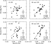 |
Fig. 5 Correlations of the residuals (individual star minus linear fit) of the [X/Fe]-[Fe/H] relations for Mg, Al, and Ti using 1D LTE (left panels) and 3D non-LTE (right panels) abundances of Mg and Al. The lines show maximum-likelihood linear fits to the data, accounting for errors in both coordinates. The values of the slope, s, the Pearson correlation coefficient, r, and the reduced chi-square of the fits are given. |
6 Discussion
This section explores possible explanations for the intrinsic dispersion of abundance ratios at a given metallicity and for correlations of the residuals in the [X/Fe] - [Fe/H] relations.
Linear regression parameters for the [X/Fe] = a + b∙ [Fe/H] + c ∙ [α/Fe] fits to our abundances.
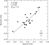 |
Fig. 6 Correlations of the residuals of the [X/Fe]-[Fe/H] fits for Y and Zr. |
6.1 Binaries and peculiar stars
Three stars in our sample have been identified as single-lined spectroscopic binaries, namely G 126-62 and G 59-27 (Latham et al. 2002) and CD –71 1234 (Ryan et al. 1999). None of them show particular large deviations from the fitted [X/Fe] - [Fe/H] relations, indicating that the components are too faint to significantly affect the derived abundance ratios. These three stars also have high values of the Gaia RUWE parameter (Castro-Ginard et al. 2024), i.e. RUWE > 1.3, indicating the presence of unresolved components. Of the remaining 22 stars in our sample, only one, LP 635-14, has a RUWE parameter suggesting the existence of an unseen component, but again there is no indication of effects on the derived [X/Fe] ratios. We conclude that the binarity of some stars in our sample is unimportant when discussing sources of the intrinsic dispersions in [X/Fe].
However, it is important to identify stars with peculiar abundances of some elements. In our sample, two stars, G 24-03 and HD 160617, belong to the class of nitrogen-rich dwarf stars. Spite et al. (2022) determined abundances for six such stars (including G 24-03 and HD 160617) relative to six ‘normal’ stars and find them to have [N/Fe] ≃ 1.0 and to be somewhat under-abundant in C and O and overabundant in Na and Al. Based on this, they suggested that the N-rich dwarfs were originally born as second-generation stars in globular clusters from gas enriched in N, Na, and Al through the CNO, Ne-Na, and Mg-Al cycles of hydrogen burning (Gratton et al. 2019). Possible first-generation gas polluters include intermediate-mass AGB stars (Ventura et al. 2001) and fast-rotating massive stars (Decressin et al. 2007). Our abundances of G 24-03 and HD 160617 agree with this scenario; Fig. 4 illustrates how they stand out by having low values of [C/Fe] and [O/Fe] and high values of [Al/Fe]. Consequently, we excluded them when fitting the [X/Fe] - [Fe/H] trends for these elements.
Another star with peculiar abundances is HD 106038. Nissen & Schuster (1997) showed that it had [X/Fe] ratios for Si, Ni, Y, and Ba enhanced by more than 0.20 dex relative to ‘normal’ halo stars with the same metallicity ([Fe/H]~ −1.4). Later Smiljanic et al. (2008) showed that the beryllium abundance of HD 106038 was enhanced by a factor of ten relative to halo dwarf stars with similar metallicity and evolutionary stage, and lithium was enhanced by a factor of two. They suggested that these enhancements were due to spallation production of Li and Be in CC SNe with exceptional high energy, so-called hypernovae (Fields et al. 2002; Nakamura & Shigeyama 2004).
Fig. 4 shows that HD 106038 stands out with [X/Fe] enhancements in C, Mg, Al, Sc, Cr, Mn, Co, Ni, Zn, Y, and Zr, exceeding three times the standard deviation of the linear fits to the [X/Fe] - [Fe/H] trends. For these elements, we excluded HD 106038 from the fits. According to the review by Nomoto et al. (2013), hypernova nucleosynthesis can explain only the enhancements of Co and Zn, while we did not observe the predicted enhancement of Ca and Ti in our abundances. The origin of the abundance pattern of HD 106038 is therefore unclear, but our precise abundances may help identify its origin.
6.2 Atomic diffusion effects
Differences in atomic diffusion of elements may contribute to the dispersion of [X/Fe] at a given metallicity even if the Teff-range of our stars is relatively small. As shown by Dotter et al. (2017), models of old metal-poor stars including atomic diffusion with radiative acceleration and turbulent mixing predict that [O/Fe] is decreased by ∼0.1 dex in turnoff stars relative to [O/Fe] in cooler main-sequence or subgiant stars, while [Ca/Fe] is enhanced in turnoff stars (see Fig. 9, lower panel in Dotter et al. 2017). Furthermore, Korn et al. (2007) and Nordlander et al. (2012), in studies of elemental abundances in turnoff and red giant stars in the globular cluster NGC 6397, found Fe to be more depleted than Ca and Ti in turnoff stars, which they ascribed to differential atomic diffusion between the elements. This interpretation was supported by calculations based on the atomic diffusion models described in Richard et al. (2005).
In view of these results, we investigated whether there is a significant dependence of the residuals in the [X/Fe]-[Fe/H] fits on effective temperature. Table 3 shows this is not the case for most elements; however, for Ca, Sc, Ti, and V, the slope of Res.[X/Fe] versus Teff has a significance greater than 2σ. As an example, Fig. 7 shows the trend of [Ca/Fe]. From Teff = 6000K to Teff = 6300 K, [Ca/Fe] increases by 0.056 dex. This is qualitatively in agreement with the predictions by Dotter et al. (2017). Furthermore, we find a negative [O/Fe]-Teff gradient, although it is only significant at the 1σ level, which is also consistent with the Dotter et al. prediction.
The effect of differential atomic diffusion on the dispersion of [X/Fe] versus [Fe/H] is, however, small. As shown in the two σfit columns in Table 3, the standard deviations of the Res. [X/Fe] = a + b · Teff fits for Ca, Sc, Ti, and V are about 10% smaller than those of the corresponding [X/Fe] = a + b · [Fe/H] fits, while for the other elements there is no significant differences. Thus, we estimate that correction for atomic diffusion effects decreases the derived intrinsic dispersions by less than about 10%, which is smaller than the estimated error of σintrin in Table 1.
Linear regressions parameters for the relation Res. [X/Fe] = a + b ∙ Teff using residuals from the [X/Fe]-[Fe/H] fits.
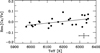 |
Fig. 7 Residuals of the [Ca/Fe]-[Fe/H] fit versus Teff. The line shows the linear regression fit to the data. |
6.3 Variations in the la/CC SN enrichment ratio
The strong correlation between the residuals of the [X/Fe]-[Fe/H] fits for the α-capture elements described in Sect. 5 suggests that the intrinsic dispersion of abundance ratios at a given [Fe/H] is connected to variations in the ratio of element production by Type Ia and CC SNe among star-forming regions. This is the canonical explanation of the difference in [X/Fe] between high-α and low-α stars found by NS10: the high-α stars were formed in situ in our Galaxy with only CC SNe contributing to the chemical evolution until a metallicity of [Fe/H]−0.7 was reached, whereas the low-α stars were accreted from dwarf galaxies (primarily from the GSE galaxy) with a slower evolution allowing significant contributions from Type Ia SNe at [Fe/H] ≳ - 1.4. We therefore see an increasing difference of [α/Fe] between high-α and low-a stars as [Fe/H] increases from –1.4 to –0.7. There is, however, evidence that Type Ia SNe begin contributing elements at a lower metallicity than [Fe/H] ≃ −1.4 in surviving dwarf spheroidal galaxies such as Fornax (Hendricks et al. 2014), Sculptor (Hill et al. 2019), and Sextans (Theler et al. 2020). Furthermore, stars in some kinematic substructures of the Galactic halo, whose progenitors are likely small dwarf galaxies, have lower [α/Fe] than GSE stars in the metallicity range –1.8 < [Fe/H] < –1.4 by as much as 0.15 dex. This includes the prograde Helmi stream (Matsuno et al. 2022a) and the high-energy, retrograde Sequoia structure (Matsuno et al. 2022b; Ceccarelli et al. 2024).
In view of these results, we investigated whether there is a correlation between [α/Fe] and the kinematics of our stars. Figure 8 shows [α/Fe] as a function of [Fe/H]. Furthermore, Fig. 9 shows the Toomre diagram with the velocity components U, Vφ, and W calculated from Gaia DR3 data as described in Nissen et al. (2021), using the same symbols as in Fig. 8. As shown, there is no obvious correlation between [α/Fe] enhancement or deficiency and the kinematics; however, a larger sample of stars is needed to test for such correlations.
We also investigated whether there is any relation between [α/Fe] and stellar age, as determined by interpolating between Yonsei-Yale isochrones (Kim et al. 2002) in the Teff- luminosity diagram using the heavy-element mass fraction Z of the star calculated from the abundances in Table A.26. Fig. 10 shows the resulting ages as a function of [Fe/H] with error bars estimated from the 1σ errors in Teff, luminosity, and Z. These error bars reflect the uncertainty on age differences relative to the standard star; the absolute ages are more uncertain because they are more sensitive to stellar-model parameters such as the mixing length. We also note that the age error varies strongly; it is large for stars on the main sequence, where the isochrones are tighter than near the turnoff.
The line shown in Fig. 10 is a linear regression fit to the ages using the inverse squared age errors as weights. The reduced chi-square of the fit is 0.92, indicating that the age scatter can be explained by the estimated errors. Nevertheless, there is a tendency for stars with slightly lower α-element abundances than the majority of stars to lie above those with higher α-element abundances. We obtained the same result using PARSEC isochrones (Bressan et al. 2012) to determine ages. The sign of this difference, which is significant at the 2-sigma level, is surprising. If the stars with lower α-element abundances were accreted from dwarf galaxies with low star formation rates, one would expect them to be younger than the stars with higher α-element abundances that are more likely to be formed in situ in regions with a high star formation rate, assuming both populations began forming stars at similar epochs. If the age difference between the stars of lower and higher α-element abundances shown in Fig. 10 is confirmed in a larger sample, it would suggest that star formation in accreted dwarf galaxies began earlier than in the Galactic halo.
A difficulty in explaining the scatter of [α/Fe] at a given [Fe/H] in terms of variations in the Ia/ CC SNe enrichment ratio is the weak correlation between the residuals of [O/Fe] and [α/Fe]. Oxygen is thought to be produced primarily in CC SNe, as are Mg, Ca, and Ti, and a correlation would therefore be expected. Fig. 11 shows that the correlation is weak, with a Pearson coefficient of 0.23 and a reduced chi-square  . If we include corrections for the Teff dependence of Res.[O/Fe] and Res.[α/Fe] (see right panel of Fig. 11), the correlation improves somewhat, but remains weak. Hence, variations in the Ia/CC SNe enrichment ratio cannot explain all the intrinsic scatter of [O/Fe].
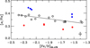 |
Fig. 8 [α/Fe] versus [Fe/H]. The line shows the linear regression to the whole sample. Stars having positive residuals (stellar [α/Fe] – linear fit) three times larger than the estimated observational error of [α/Fe] (σobs = 0.013 dex) are shown with filled blue circles and those with Δ < 3σobs are shown with filled red circles The rest of the stars are shown with open circles. |
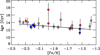 |
Fig. 10 Stellar age as a function of [Fe/H] using the same symbols as in Fig. 8, with 1-sigma error bars on the ages. The line shows the linear regression fit to all stars, weighted by the inverse squared age errors. |
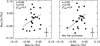 |
Fig. 11 Correlations of the residuals of the [O/Fe]-[Fe/H] and [α/Fe]-[Fe/H] fits. In the right panel, the residuals are corrected for their Teff dependence. |
6.4 Stochastic effects in sampling the IMF of CC SNe
Because the [X/Fe] yields from CC SNe depend strongly on stellar mass, stochastic sampling of the IMF will introduce scatter in abundance ratios at a given [Fe/H] between star-forming regions. Following the method of Griffith et al. (2023), we calculated the standard deviation of [X/Fe] as a function of the number of CC SNe, NCCSN, enriching a star-forming region. This was done by repeating the sampling 10000 times, randomly drawing SNe with progenitor masses between 13 and 80 M⊙ from a Salpeter (1955) IMF weighted distribution (see Fig. 12 for an example). We adopted yields corresponding to [Fe/H] = –2.0 from Limongi & Chieffi (2018) using either their ‘set M’ yields, for which the whole mass of a SN is expelled, or their ‘set R’ yields, in which SNe with M > 25M⊙ are assumed to collapse into black holes and therefore only contribute to the yields via stellar winds. In both cases, yields are available for initial stellar rotational velocities Vrot = 0, 150, and 300 km s−1.
Fig. 12 shows that the best agreement between the predicted and measured dispersions of [X/Fe] is obtained for NCCSN between 30 and 100. Excluding Co and Ni, for which there is no significant variation in the calculated dispersion, and noting that the calculated dispersion scales as  , the data suggest a weighted mean value of 〈NCCSN〉 = 64 ± 14. We obtain a similar number for ‘set M’ yields, corresponding to Vrot = 0 and 150 km s−1and also when using the yields corresponding to [Fe/H] = –3.0. ‘Set R’ yields suggest a somewhat smaller value, typically NCCSN ≃ 50. Griffith et al. (2023) obtain a similar number. Although their derived intrinsic dispersions are about a factor of two larger than ours, this is compensated by their use of solar-metallicity yields from Sukhbold et al. (2016), which lead to larger standard deviations of [X/Fe] for a given number of SNe than the yields of Limongi & Chieffi (2018). As discussed by Griffith et al. (2023, see their Eq. (6)), the region over which the products of 50 CC SNe are mixed must have a gas mass of about 105 M⊙ in order to reach an oxygen abundance similar to that of our stars. Interestingly, this is a typical mass of giant molecular clouds (Fukui & Kawamura 2010).
6.5 Yttrium and zirconium
Yttrium (Y) and Zr belong to the group of light neutron-capture elements, which also includes strontium. At the metallicities of our stars, these elements are likely produced by both the r-process and the weak s-process in massive stars, although we cannot exclude a contribution from the main s-process in low-mass (M = 1 – 3M⊙) AGB stars (Cristallo et al. 2011). Table 1 shows that the intrinsic dispersion for [Y/Fe] and [Zr/Fe] as a function of [Fe/H] is about a factor of two higher than the dispersion for the α-elements. Li et al. (2022) obtain a similar result for a larger sample of halo stars with –3.5 < [Fe/H] < –2.0. They also find a strong correlation between the residuals for Y and Zr, similar to Fig. 6, indicating that both elements originate from the same nucleosynthetic processes. It should also be noted that Griffith et al. (2026) recently measured the dispersion of several neutron-capture elements in their sample of 86 subgiant stars with –2.0 < [Fe/H] < –1.0. For [Y/Fe] and [Zr/Fe], they find intrinsic dispersions of 0.20 dex and 0.17 dex, respectively, which are about a factor of two larger than our value of 0.09 dex.
Based on the stochastic chemical evolution model of Cescutti (2008), Cescutti & Chiappini (2014) showed that the large scatter of neutron-capture elements in metal-poor halo stars can be explained by combining the weak s-process in fast-rotating stars with various r-process scenarios in massive stars. Scannapieco et al. (2022) simulated these processes in a hydrodynamical cosmological model that also includes the formation of the α elements and accretion from dwarf galaxies. Interestingly, the model predicts that the ratio of the scatter of [Sr/Fe] is about twice as large as that in [Mg/Fe] (see Fig. 9 in Scannapieco et al. 2022), in agreement with the ratio of the intrinsic dispersions in our Table 1.
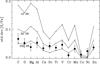 |
Fig. 12 Calculated standard deviations of [X/Fe] as a function of the number of CC SNe enriching a star-forming region (open circles connected by lines) for ‘set M’ yields from Limongi & Chieffi (2018) corresponding to [Fe/H] = −2.0 and Vrot = 300 km s−1, compared with the intrinsic dispersion (filled circles with error bars) of the [X/Fe]-[Fe/H] trends. |
7 Summary and conclusions
Based on VLT/UVES blue spectra, we determined abundance ratios in a sample of 25 halo stars with –2.4 < [Fe/H] < –1.3 belonging to the turnoff region of the HR diagram. As the spectra have S/N ≳ 200, and we derived Teff from Hß line profiles and log g from Gaia parallaxes, we kept the errors of the differential [X/Fe] values at a level of 0.02-0.04 dex, which allowed us to determine reliable values of the intrinsic dispersion in linear fits of [X/Fe] as a function of [Fe/H]. The derived dispersions are smaller than those found in previous investigations (Belokurov & Kravtsov 2022; Griffith et al. 2023, 2026), and the correlations between the residuals in the fits for different elements provide useful constraints on possible explanations for the intrinsic dispersions.
We derived abundances using a 1D LTE model-atmosphere analysis of measured equivalent widths of spectral lines. We applied 3D non-LTE corrections to C, O, Mg, Al, and Ca, for which only neutral atomic lines were available, and 3D LTE corrections to Ti and Fe, for which lines of ionised species were used. The corrections affect the slopes of the [X/Fe]-[Fe/H] relations, but have limited effects on the scatter at a given [Fe/H], which can be attributed to the relatively small range in Teff and log g for our sample of stars. For Mg and Al, the 3D non-LTE corrections are nevertheless important for the correlations between residuals in the [X/Fe]-[Fe/H] fits and those of other elements (Fig. 5). It would therefore be important to obtain 3D non-LTE corrections for the remaining elements, especially Mn, Co, Ni, and Zn, for which only lines from neutral atoms are available.
Correlations between residuals in the [X/Fe]-[Fe/H] fits and effective temperature suggest that differential atomic diffusion, including radiative acceleration, has a significant effect on [Ca/Fe], [Sc/Fe], [Ti/Fe], and [V/Fe]. However, the effect is small over the narrow Teff range of our stars and contributes at most 10% to the intrinsic scatter of the abundance ratios.
Variations in the Ia / CC SNe enrichment ratio between starforming regions in the Milky Way halo and dwarf galaxies may explain the intrinsic scatter in the [X/Fe]-[Fe/H] relations. This is indeed the canonical explanation for the striking difference between high-α and low-α stars at metallicities [Fe/H] > –1.3. At lower metallicities, such as those considered here, there is evidence that variations in [α/Fe] remain significant; this may extend down to [Fe/H]~ −2.0 for stars with extreme kinematics (Matsuno et al. 2022a,b; Ceccarelli et al. 2024). Correlations between the residuals of [X/Fe] for Mg, Al, Ca, and Ti (Table 2 and Fig. 5) support this scenario, but the lack of a clear correlation between the residuals for oxygen and those of the α-elements (Fig. 11) is puzzling, and there is no obvious correlation between the kinematics of our stars and [α/Fe] (Fig. 9). Clearly, a larger sample of halo stars with high-precision abundances is needed to investigate these issues further.
Another possible explanation for the intrinsic scatter in the [X/Fe]-[Fe/H] relations is stochastic effects in sampling the IMF of CC SNe in star-forming regions. Nissen et al. (1994) also discussed such effects, using upper limits on the scatter of [O/Fe], [Mg/Fe], and [Ca/Fe] in nine metal-poor halo stars, and estimated that NCCSN ≳ 20 is required to reproduce the observed scatters. In Sect. 6.4, we used the yields from Limongi & Chieffi (2018) to estimate that NCCSN ∼ 50-70 is required to explain the small intrinsic scatter of [X/Fe] derived in this work (Fig. 12). Griffith et al. (2023) estimate a similar number of CC SNe from the scatter of abundance ratios in 86 subgiant stars, and show that this implies that CC SNe ejecta are mixed over a gas mass of ∼105M⊙, comparable to the typical mass of giant molecular clouds.
Among the iron-peak elements (Cr, Mn, Ni, Co, and Zn), Nissen & Schuster (2010, 2011) found differences in [Ni/Fe] and [Zn/Fe] between high-α and low-α halo stars at [Fe/H] > –1.3. However, for the present sample of more metal-poor stars, we find no correlation of [Ni/Fe] and [Zn/Fe] with [α/Fe] (Table 2 compared with Table 1). Conversely, predictions of the stochastic effect for iron-peak elements agree with the derived intrinsic dispersions of the [X/Fe]-[Fe/H] fits, predicting higher values for Mn and Zn than for Cr, Co, and Ni (Fig. 12). However, 3D non-LTE corrections for the iron-peak elements should be taken into account before firm conclusions can be drawn.
It is likely that both variations in the Ia / CC SNe enrichment ratio and stochastic effects in sampling the IMF contribute to the scatter in the [X/Fe]-[Fe/H] relations. The small intrinsic scatter that we have determined for the metallicity range –2.4 < [Fe/H] < –1.3 places important constraints on these effects and also constrains other possible sources of the scatter, such as variations in the IMF between star-forming regions (Bastian et al. 2010) and bursts of star formation (Gilmore & Wyse 1991).
Acknowledgements
We thank Bengt Gustafsson for very useful comments on a first version of this paper, and the referee is thanked for many detailed suggestions that helped to clarify the text. A.M.A. acknowledges support from the Swedish Research Council (VR 2020-03940, VR 2025-05167), and the Crafoord Foundation via the Royal Swedish Academy of Sciences (CR 2024-0015). This research was supported by computational resources provided by the Australian Government through the National Computational Infrastructure (NCI) under the National Computational Merit Allocation Scheme and the ANU Merit Allocation Scheme (project y89). The computations were also made possible thanks to resources at the National Supercomputing Centre (NSC, Tetralith cluster) provided by the National Academic Infrastructure for Supercomputing in Sweden (NAISS), partially funded by the Swedish Research Council through grant agreement no. 2022-06725. This research has made use of data from the European Space Agency (ESA) mission Gaia (https://www.cosmos.esa.int/gaia), processed by the Gaia Data Processing and Analysis Consortium (DPAC, https://www.cosmos.esa.int/web/gaia/dpac/consortium). Funding for the DPAC has been provided by national institutions, in particular the institutions participating in the Gaia Multilateral Agreement. This research has made use of the SIMBAD database operated at CDS, Strasbourg, France (Wenger et al. 2000).
References
- Adibekyan, V. Z., Sousa, S. G., Santos, N. C., et al. 2012, A&A, 545, A32 [NASA ADS] [CrossRef] [EDP Sciences] [Google Scholar]
- Akerman, C.J., Carigi, L., Nissen, P. E., Pettini, M., & Asplund, M. 2004, A&A, 414, 931 [NASA ADS] [CrossRef] [EDP Sciences] [Google Scholar]
- Amarsi, A. M., Lind, K., Asplund, M., Barklem, P. S., & Collet, R. 2016, MNRAS, 463, 1518 [NASA ADS] [CrossRef] [Google Scholar]
- Amarsi, A. M., Barklem, P. S., Asplund, M., Collet, R., & Zatsarinny, O. 2018a, A&A, 616, A89 [NASA ADS] [CrossRef] [EDP Sciences] [Google Scholar]
- Amarsi, A. M., Nordlander, T., Barklem, P. S., et al. 2018b, A&A, 615, A139 [NASA ADS] [CrossRef] [EDP Sciences] [Google Scholar]
- Amarsi, A. M., Barklem, P. S., Collet, R., Grevesse, N., & Asplund, M. 2019a, A&A, 624, A111 [NASA ADS] [CrossRef] [EDP Sciences] [Google Scholar]
- Amarsi, A. M., Nissen, P. E., Asplund, M., Lind, K., & Barklem, P. S. 2019b, A&A, 622, L4 [NASA ADS] [CrossRef] [EDP Sciences] [Google Scholar]
- Amarsi, A. M., Nissen, P. E., & Skúladóttir, Á. 2019c, A&A, 630, A104 [NASA ADS] [CrossRef] [EDP Sciences] [Google Scholar]
- Amarsi, A. M., Grevesse, N., Asplund, M., & Collet, R. 2021, A&A, 656, A113 [NASA ADS] [CrossRef] [EDP Sciences] [Google Scholar]
- Amarsi, A. M., Liljegren, S., & Nissen, P. E. 2022, A&A, 668, A68 [NASA ADS] [CrossRef] [EDP Sciences] [Google Scholar]
- Argast, D., Samland, M., Gerhard, O. E., & Thielemann, F. K. 2000, A&A, 356, 873 [Google Scholar]
- Argast, D., Samland, M., Thielemann, F. K., & Gerhard, O. E. 2002, A&A, 388, 842 [NASA ADS] [CrossRef] [EDP Sciences] [Google Scholar]
- Arnone, E., Ryan, S. G., Argast, D., Norris, J. E., & Beers, T. C. 2005, A&A, 430, 507 [NASA ADS] [CrossRef] [EDP Sciences] [Google Scholar]
- Asplund, M., Amarsi, A. M., & Grevesse, N. 2021, A&A, 653, A141 [NASA ADS] [CrossRef] [EDP Sciences] [Google Scholar]
- Audouze, J., & Silk, J. 1995, ApJ, 451, L49 [Google Scholar]
- Barklem, P. S. 2016, A&A Rev., 24, 9 [Google Scholar]
- Barklem, P. S., Stempels, H. C., Allende Prieto, C., et al. 2002, A&A, 385, 951 [NASA ADS] [CrossRef] [EDP Sciences] [Google Scholar]
- Barklem, P. S., Amarsi, A. M., Grumer, J., et al. 2021, ApJ, 908, 245 [NASA ADS] [CrossRef] [Google Scholar]
- Bastian, N., Covey, K. R., & Meyer, M. R. 2010, ARA&A, 48, 339 [Google Scholar]
- Belokurov, V., & Kravtsov, A. 2022, MNRAS, 514, 689 [NASA ADS] [CrossRef] [Google Scholar]
- Biemont, E., & Godefroid, M. 1980, A&A, 84, 361 [NASA ADS] [Google Scholar]
- Booth, A. J., Blackwell, D. E., Petford, A. D., & Shallis, M. J. 1984, MNRAS, 208, 147 [NASA ADS] [CrossRef] [Google Scholar]
- Botnen, A., & Carlsson, M. 1999, Astrophys. Space Sci. Lib., 240, 379 [NASA ADS] [CrossRef] [Google Scholar]
- Bressan, A., Marigo, P., Girardi, L., et al. 2012, MNRAS, 427, 127 [NASA ADS] [CrossRef] [Google Scholar]
- Brown, J. M., & Evenson, K. M. 1999, Phys. Rev. A, 60, 956 [Google Scholar]
- Caliskan, S., Amarsi, A. M., Racca, M., et al. 2025, A&A, 696, A210 [NASA ADS] [CrossRef] [EDP Sciences] [Google Scholar]
- Casagrande, L., Ramírez, I., Meléndez, J., Bessell, M., & Asplund, M. 2010, A&A, 512, A54 [NASA ADS] [CrossRef] [EDP Sciences] [Google Scholar]
- Castro-Ginard, A., Penoyre, Z., Casey, A. R., et al. 2024, A&A, 688, A1 [NASA ADS] [CrossRef] [EDP Sciences] [Google Scholar]
- Cayrel, R., Depagne, E., Spite, M., et al. 2004, A&A, 416, 1117 [NASA ADS] [CrossRef] [EDP Sciences] [Google Scholar]
- Ceccarelli, E., Massari, D., Mucciarelli, A., et al. 2024, A&A, 684, A37 [NASA ADS] [CrossRef] [EDP Sciences] [Google Scholar]
- Cescutti, G. 2008, A&A, 481, 691 [NASA ADS] [CrossRef] [EDP Sciences] [Google Scholar]
- Cescutti, G., & Chiappini, C. 2014, A&A, 565, A51 [NASA ADS] [CrossRef] [EDP Sciences] [Google Scholar]
- Cohen, J. G., Christlieb, N., McWilliam, A., et al. 2004, ApJ, 612, 1107 [CrossRef] [Google Scholar]
- Cristallo, S., Piersanti, L., Straniero, O., et al. 2011, ApJS, 197, 17 [NASA ADS] [CrossRef] [Google Scholar]
- Cutri, R. M., Skrutskie, M. F., van Dyk, S., et al. 2003, VizieR Online Data Catalog: II/246 [Google Scholar]
- Decressin, T., Charbonnel, C., & Meynet, G. 2007, A&A, 475, 859 [CrossRef] [EDP Sciences] [Google Scholar]
- Den Hartog, E. A., Lawler, J. E., Sneden, C., et al. 2021, ApJS, 255, 27 [NASA ADS] [CrossRef] [Google Scholar]
- Dotter, A., Conroy, C., Cargile, P., & Asplund, M. 2017, ApJ, 840, 99 [Google Scholar]
- Edvardsson, B., Andersen, J., Gustafsson, B., et al. 1993, A&A, 275, 101 [NASA ADS] [Google Scholar]
- Ernandes, H., Skúladóttir, Á., Feltzing, S., & Feuillet, D. 2025, A&A, 703, A256 [NASA ADS] [CrossRef] [EDP Sciences] [Google Scholar]
- Ezzeddine, R., Merle, T., Plez, B., et al. 2018, A&A, 618, A141 [NASA ADS] [CrossRef] [EDP Sciences] [Google Scholar]
- Fabbian, D., Nissen, P. E., Asplund, M., Pettini, M., & Akerman, C. 2009, A&A, 500, 1143 [NASA ADS] [CrossRef] [EDP Sciences] [Google Scholar]
- Fields, B. D., Daigne, F., Cassé, M., & Vangioni-Flam, E. 2002, ApJ, 581, 389 [NASA ADS] [CrossRef] [Google Scholar]
- Fuhrmann, K. 1998, A&A, 338, 161 [NASA ADS] [Google Scholar]
- Fukui, Y., & Kawamura, A. 2010, ARA&A, 48, 547 [Google Scholar]
- Gaia Collaboration (Vallenari, A., et al.) 2023, A&A, 674, A1 [NASA ADS] [CrossRef] [EDP Sciences] [Google Scholar]
- García Pérez, A. E., Allende Prieto, C., Holtzman, J. A., et al. 2016, AJ, 151, 144 [Google Scholar]
- Gilmore, G., & Wyse, R. F. G. 1991, ApJ, 367, L55 [NASA ADS] [CrossRef] [Google Scholar]
- Giribaldi, R. E., da Silva, A. R., Smiljanic, R., & Cornejo Espinoza, D. 2021, A&A, 650, A194 [NASA ADS] [CrossRef] [EDP Sciences] [Google Scholar]
- Gratton, R. G., Carretta, E., Matteucci, F., & Sneden, C. 2000, A&A, 358, 671 [NASA ADS] [Google Scholar]
- Gratton, R., Bragaglia, A., Carretta, E., et al. 2019, A&A Rev., 27, 8 [Google Scholar]
- Greenlee, T. R., & Whaling, W. 1979, J. Quant. Spec. Radiat. Transf., 21, 55 [Google Scholar]
- Griffith, E. J., Johnson, J. A., Weinberg, D. H., et al. 2023, ApJ, 944, 47 [NASA ADS] [CrossRef] [Google Scholar]
- Griffith, E. J., Blum, M., Weinberg, D. H., et al. 2026, ApJ, 1001, 193 [Google Scholar]
- Gustafsson, B., Edvardsson, B., Eriksson, K., et al. 2008, A&A, 486, 951 [NASA ADS] [CrossRef] [EDP Sciences] [Google Scholar]
- Hannaford, P., Lowe, R. M., Grevesse, N., Biemont, E., & Whaling, W. 1982, ApJ, 261, 736 [NASA ADS] [CrossRef] [Google Scholar]
- Hawkins, K., Jofré, P., Masseron, T., & Gilmore, G. 2015, MNRAS, 453, 758 [NASA ADS] [CrossRef] [Google Scholar]
- Hayek, W., Asplund, M., Collet, R., & Nordlund, Â. 2011, A&A, 529, A158 [NASA ADS] [CrossRef] [EDP Sciences] [Google Scholar]
- Hayes, C. R., Majewski, S. R., Shetrone, M., et al. 2018, ApJ, 852, 49 [NASA ADS] [CrossRef] [Google Scholar]
- Helmi, A. 2020, ARA&A, 58, 205 [Google Scholar]
- Hendricks, B., Koch, A., Walker, M., et al. 2014, A&A, 572, A82 [NASA ADS] [CrossRef] [EDP Sciences] [Google Scholar]
- Hill, V., Skúladóttir, Á., Tolstoy, E., et al. 2019, A&A, 626, A15 [NASA ADS] [CrossRef] [EDP Sciences] [Google Scholar]
- Jönsson, P., & Froese Fischer, C. 1997, J. Phys. B Atom. Mol. Phys., 30, 5861 [Google Scholar]
- Karlsson, T. 2005, A&A, 439, 93 [NASA ADS] [CrossRef] [EDP Sciences] [Google Scholar]
- Karlsson, T., & Gustafsson, B. 2005, A&A, 436, 879 [NASA ADS] [CrossRef] [EDP Sciences] [Google Scholar]
- Kim, Y.-C., Demarque, P., Yi, S. K., & Alexander, D. R. 2002, ApJS, 143, 499 [Google Scholar]
- Korn, A. J., Grundahl, F., Richard, O., et al. 2007, ApJ, 671, 402 [NASA ADS] [CrossRef] [Google Scholar]
- Kostyk, R. I. 1982, Astrometriia i Astrofizika, 46, 58 [Google Scholar]
- Kostyk, R. I., & Orlova, T. V. 1983, Astrometriia i Astrofizika, 49, 39 [Google Scholar]
- Kramida, A., Yu. Ralchenko, Reader, J., & and NIST ASD Team 2024, NIST Atomic Spectra Database (ver. 5.12). Available: https://physics.nist.gov/asd. National Institute of Standards and Technology, Gaithersburg, MD. [Google Scholar]
- Lagae, C., Amarsi, A. M., Rodríguez Díaz, L. F., et al. 2023, A&A, 672, A90 [NASA ADS] [CrossRef] [EDP Sciences] [Google Scholar]
- Latham, D. W., Stefanik, R. P., Torres, G., et al. 2002, AJ, 124, 1144 [NASA ADS] [CrossRef] [Google Scholar]
- Lawler, J. E., Sneden, C., & Cowan, J. J. 2015, ApJS, 220, 13 [NASA ADS] [CrossRef] [Google Scholar]
- Lawler, J. E., Sneden, C., Nave, G., et al. 2017, ApJS, 228, 10 [CrossRef] [Google Scholar]
- Lawler, J. E., Hala, Sneden, C., et al. 2019, ApJS, 241, 21 [NASA ADS] [CrossRef] [Google Scholar]
- Leenaarts, J., & Carlsson, M. 2009, ASP Conf. Ser., 415, 87 [Google Scholar]
- Li, H., Aoki, W., Matsuno, T., et al. 2022, ApJ, 931, 147 [NASA ADS] [CrossRef] [Google Scholar]
- Limongi, M., & Chieffi, A. 2018, ApJS, 237, 13 [NASA ADS] [CrossRef] [Google Scholar]
- Lind, K., Bergemann, M., & Asplund, M. 2012, MNRAS, 427, 50 [Google Scholar]
- Lind, K., Nordlander, T., Wehrhahn, A., et al. 2022, A&A, 665, A33 [NASA ADS] [CrossRef] [EDP Sciences] [Google Scholar]
- Ljung, G., Nilsson, H., Asplund, M., & Johansson, S. 2006, A&A, 456, 1181 [NASA ADS] [CrossRef] [EDP Sciences] [Google Scholar]
- Ludwig, H. G., & Steffen, M. 2016, Astron. Nachr., 337, 844 [NASA ADS] [CrossRef] [Google Scholar]
- Magic, Z., Collet, R., Asplund, M., et al. 2013, A&A, 557, A26 [NASA ADS] [CrossRef] [EDP Sciences] [Google Scholar]
- Mallinson, J. W. E., Lind, K., Amarsi, A. M., et al. 2022, A&A, 668, A103 [NASA ADS] [CrossRef] [EDP Sciences] [Google Scholar]
- Mallinson, J. W. E., Lind, K., Amarsi, A. M., et al. 2023, A&A, 673, C1 [NASA ADS] [CrossRef] [EDP Sciences] [Google Scholar]
- Mallinson, J. W. E., Lind, K., Amarsi, A. M., & Youakim, K. 2024, A&A, 687, A5 [NASA ADS] [CrossRef] [EDP Sciences] [Google Scholar]
- Matsuno, T., Dodd, E., Koppelman, H. H., et al. 2022a, A&A, 665, A46 [NASA ADS] [CrossRef] [EDP Sciences] [Google Scholar]
- Matsuno, T., Koppelman, H. H., Helmi, A., et al. 2022b, A&A, 661, A103 [NASA ADS] [CrossRef] [EDP Sciences] [Google Scholar]
- Matsuno, T., Amarsi, A. M., Carlos, M., & Nissen, P. E. 2024, A&A, 688, A72 [NASA ADS] [CrossRef] [EDP Sciences] [Google Scholar]
- McWilliam, A., Preston, G. W., Sneden, C., & Searle, L. 1995, AJ, 109, 2757 [Google Scholar]
- Meléndez, J., & Barbuy, B. 2009, A&A, 497, 611 [NASA ADS] [CrossRef] [EDP Sciences] [Google Scholar]
- Nakamura, K., & Shigeyama, T. 2004, ApJ, 610, 888 [Google Scholar]
- Nissen, P. E., & Gustafsson, B. 2018, A&A Rev., 26, 6 [Google Scholar]
- Nissen, P. E., & Schuster, W. J. 1997, A&A, 326, 751 [NASA ADS] [Google Scholar]
- Nissen, P. E., & Schuster, W. J. 2010, A&A, 511, L10 [NASA ADS] [CrossRef] [EDP Sciences] [Google Scholar]
- Nissen, P. E., & Schuster, W. J. 2011, A&A, 530, A15 [NASA ADS] [CrossRef] [EDP Sciences] [Google Scholar]
- Nissen, P. E., Gustafsson, B., Edvardsson, B., & Gilmore, G. 1994, A&A, 285, 440 [NASA ADS] [Google Scholar]
- Nissen, P. E., Primas, F., Asplund, M., & Lambert, D. L. 2002, A&A, 390, 235 [NASA ADS] [CrossRef] [EDP Sciences] [Google Scholar]
- Nissen, P. E., Chen, Y. Q., Asplund, M., & Pettini, M. 2004, A&A, 415, 993 [NASA ADS] [CrossRef] [EDP Sciences] [Google Scholar]
- Nissen, P. E., Akerman, C., Asplund, M., et al. 2007, A&A, 469, 319 [NASA ADS] [CrossRef] [EDP Sciences] [Google Scholar]
- Nissen, P. E., Silva-Cabrera, J. S., & Schuster, W. J. 2021, A&A, 651, A57 [NASA ADS] [CrossRef] [EDP Sciences] [Google Scholar]
- Nomoto, K., Kobayashi, C., & Tominaga, N. 2013, ARA&A, 51, 457 [Google Scholar]
- Nordlander, T., & Lind, K. 2017, A&A, 607, A75 [NASA ADS] [CrossRef] [EDP Sciences] [Google Scholar]
- Nordlander, T., Korn, A. J., Richard, O., & Lind, K. 2012, ApJ, 753, 48 [NASA ADS] [CrossRef] [Google Scholar]
- Pehlivan Rhodin, A., Hartman, H., Nilsson, H., & Jönsson, P. 2017, A&A, 598, A102 [NASA ADS] [CrossRef] [EDP Sciences] [Google Scholar]
- Reggiani, H., Meléndez, J., Kobayashi, C., Karakas, A., & Placco, V. 2017, A&A, 608, A46 [NASA ADS] [CrossRef] [EDP Sciences] [Google Scholar]
- Richard, O., Michaud, G., & Richer, J. 2005, ApJ, 619, 538 [Google Scholar]
- Roberts, J. R., Andersen, T., & Sorensen, G. 1973, ApJ, 181, 567 [Google Scholar]
- Rodríguez Díaz, L. F., Lagae, C., Amarsi, A. M., et al. 2024, A&A, 688, A212 [NASA ADS] [CrossRef] [EDP Sciences] [Google Scholar]
- Ryan, S. G., Norris, J. E., & Beers, T. C. 1999, ApJ, 523, 654 [CrossRef] [Google Scholar]
- Salpeter, E. E. 1955, ApJ, 121, 161 [Google Scholar]
- Scannapieco, C., Cescutti, G., & Chiappini, C. 2022, MNRAS, 516, 6075 [NASA ADS] [CrossRef] [Google Scholar]
- Schuster, W. J., & Nissen, P. E. 1989, A&A, 221, 65 [NASA ADS] [Google Scholar]
- Shetrone, M., Bizyaev, D., Lawler, J. E., et al. 2015, ApJS, 221, 24 [Google Scholar]
- Skúladóttir, Á., Ernandes, H., Feuillet, D. K., et al. 2025, ApJ, 986, L21 [Google Scholar]
- Smiljanic, R., Pasquini, L., Primas, F., et al. 2008, MNRAS, 385, L93 [NASA ADS] [CrossRef] [Google Scholar]
- Spite, M., Spite, F., Caffau, E., Bonifacio, P., & François, P. 2022, A&A, 667, A139 [NASA ADS] [CrossRef] [EDP Sciences] [Google Scholar]
- Stein, R. F., Nordlund, Â., Collet, R., & Trampedach, R. 2024, ApJ, 970, 24 [NASA ADS] [CrossRef] [Google Scholar]
- Sukhbold, T., Ertl, T., Woosley, S. E., Brown, J. M., & Janka, H.-T. 2016, ApJ, 821, 38 [Google Scholar]
- Theler, R., Jablonka, P., Lucchesi, R., et al. 2020, A&A, 642, A176 [NASA ADS] [CrossRef] [EDP Sciences] [Google Scholar]
- Unsöld, A. 1955, Physik der Sternatmospharen, MIT besonderer Berucksichtigung der Sonne. (Berlin: Springer) [Google Scholar]
- Ventura, P., D’Antona, F., Mazzitelli, I., & Gratton, R. 2001, ApJ, 550, L65 [CrossRef] [Google Scholar]
- Wenger, M., Ochsenbein, F., Egret, D., et al. 2000, A&AS, 143, 9 [NASA ADS] [Google Scholar]
- Wood, M. P., Lawler, J. E., Sneden, C., & Cowan, J. J. 2013, ApJS, 208, 27 [NASA ADS] [CrossRef] [Google Scholar]
- Wood, M. P., Lawler, J. E., Den Hartog, E. A., Sneden, C., & Cowan, J. J. 2014a, ApJS, 214, 18 [Google Scholar]
- Wood, M. P., Lawler, J. E., Sneden, C., & Cowan, J. J. 2014b, ApJS, 211, 20 [NASA ADS] [CrossRef] [Google Scholar]
- Yi, S. K., Kim, Y.-C., & Demarque, P. 2003, ApJS, 144, 259 [Google Scholar]
For two elements, X and Y, with number densities NX and NY, [X/Y] ≡ log(NX/NY)star – log(NX/NY)⊙.
We verified that linear interpolation errors in the MARCS grid affect the dispersion of the [X/Fe]-[Fe/H] relations by less than 0.003 dex.
For the elements Al, Co, and Zr with only one line available, we estimated σX,line from the error of the EW corresponding to the S/N of the spectrum.
When fitting [X/Fe] for Mg, Ca, or Ti, the element itself is not included in the calculation of [α/Fe].
For the elements N, Ne, and Si, which make a significant contribution to Z and are missing in Table A.2, we assumed that [Ne/Fe] and [Si/Fe] are equal to [α/Fe] and that [N/Fe]= 0.0 except for the two nitrogen-rich stars, G 24-03 and HD 160617, for which [N/Fe]=1.0 was adopted.
Appendix A Atomic data and derived abundances
List of spectral lines.
All Tables
Linear regression parameters for the [X/Fe] = a + b∙ [Fe/H] + c ∙ [α/Fe] fits to our abundances.
Linear regressions parameters for the relation Res. [X/Fe] = a + b ∙ Teff using residuals from the [X/Fe]-[Fe/H] fits.
All Figures
|
Fig. 1 Comparison of Ca, Ti, and Fe lines in spectra of two stars with similar atmospheric parameters and abundances. The spectrum of G59-27 (Teff = 6232K, log g = 4.22, [Fe/H] = −1.90, [Ca/Fe] = 0.42, and [Ti/Fe] = 0.33) is shown in blue, and that of CD–3018140 (Teff = 6241K, log g = 4.15, [Fe/H] = −1.84, [Ca/Fe] = 0.42, and [Ti/Fe] = 0.34) in red. For each line the measured equivalent widths for the two stars are given in mÅ with an estimated uncertainty of ±0.6 mÅ. |
| In the text | |
|
Fig. 2 Comparison of effective temperatures determined by Giribaldi et al. (2021) from Hα profiles and those of Amarsi et al. (2019b) from Hβ profiles. |
| In the text | |
|
Fig. 3 Difference in Mg abundances derived from the 4703.0 and 4571.1 Å lines as a function of [Fe/H] normalised to zero for the standard star, HD 110621. |
| In the text | |
|
Fig. 4 Trends of [X/Fe] as a function of [Fe/H] for 15 elements. Each panel shows the atomic species of the spectral lines used for abundance determinations and the method of analysis. Straight lines show least-squares fits to stars marked by filled black circles. Stars marked by filled red circles for some elements are considered peculiar and are not included in the fits. In the Al, Y, and Zr panels, HD 106038 lies above the upper frame, as indicated by a red arrow. Error bars shown in this and the following figures refer to the values of σobs given in Table 1. |
| In the text | |
|
Fig. 5 Correlations of the residuals (individual star minus linear fit) of the [X/Fe]-[Fe/H] relations for Mg, Al, and Ti using 1D LTE (left panels) and 3D non-LTE (right panels) abundances of Mg and Al. The lines show maximum-likelihood linear fits to the data, accounting for errors in both coordinates. The values of the slope, s, the Pearson correlation coefficient, r, and the reduced chi-square of the fits are given. |
| In the text | |
|
Fig. 6 Correlations of the residuals of the [X/Fe]-[Fe/H] fits for Y and Zr. |
| In the text | |
|
Fig. 7 Residuals of the [Ca/Fe]-[Fe/H] fit versus Teff. The line shows the linear regression fit to the data. |
| In the text | |
|
Fig. 8 [α/Fe] versus [Fe/H]. The line shows the linear regression to the whole sample. Stars having positive residuals (stellar [α/Fe] – linear fit) three times larger than the estimated observational error of [α/Fe] (σobs = 0.013 dex) are shown with filled blue circles and those with Δ < 3σobs are shown with filled red circles The rest of the stars are shown with open circles. |
| In the text | |
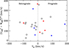 |
Fig. 9 Toomre diagram using the same symbols as defined in Fig. 8. |
| In the text | |
|
Fig. 10 Stellar age as a function of [Fe/H] using the same symbols as in Fig. 8, with 1-sigma error bars on the ages. The line shows the linear regression fit to all stars, weighted by the inverse squared age errors. |
| In the text | |
|
Fig. 11 Correlations of the residuals of the [O/Fe]-[Fe/H] and [α/Fe]-[Fe/H] fits. In the right panel, the residuals are corrected for their Teff dependence. |
| In the text | |
|
Fig. 12 Calculated standard deviations of [X/Fe] as a function of the number of CC SNe enriching a star-forming region (open circles connected by lines) for ‘set M’ yields from Limongi & Chieffi (2018) corresponding to [Fe/H] = −2.0 and Vrot = 300 km s−1, compared with the intrinsic dispersion (filled circles with error bars) of the [X/Fe]-[Fe/H] trends. |
| In the text | |
Current usage metrics show cumulative count of Article Views (full-text article views including HTML views, PDF and ePub downloads, according to the available data) and Abstracts Views on Vision4Press platform.
Data correspond to usage on the plateform after 2015. The current usage metrics is available 48-96 hours after online publication and is updated daily on week days.
Initial download of the metrics may take a while.