


| Issue |
A&A
Volume 711, July 2026
|
|
|---|---|---|
| Article Number | A285 | |
| Number of page(s) | 24 | |
| Section | Extragalactic astronomy | |
| DOI | https://doi.org/10.1051/0004-6361/202558490 | |
| Published online | 23 July 2026 | |
Euclid Quick Data Release (Q1)
XXXVIII. Euclid spectroscopy of quasars. 1. Identification and redshift determination of 3500 bright quasars
1
Leiden Observatory, Leiden University, Einsteinweg 55, 2333 CC, Leiden, The Netherlands
2
Kapteyn Astronomical Institute, University of Groningen, PO Box 800, 9700 AV, Groningen, The Netherlands
3
Cosmic Dawn Center (DAWN)
4
INAF-Osservatorio di Astrofisica e Scienza dello Spazio di Bologna, Via Piero Gobetti 93/3, 40129 Bologna, Italy
5
Dipartimento di Fisica e Astronomia, Università di Firenze, Via G. Sansone 1, 50019 Sesto Fiorentino, Firenze, Italy
6
University of Trento, Via Sommarive 14, I-38123 Trento, Italy
7
INAF-Osservatorio Astrofisico di Arcetri, Largo E. Fermi 5, 50125 Firenze, Italy
8
SRON Netherlands Institute for Space Research, Landleven 12, 9747 AD, Groningen, The Netherlands
9
School of Physics & Astronomy, University of Southampton, Highfield Campus, Southampton SO17 1BJ, UK
10
Max-Planck-Institut für Astronomie, Königstuhl 17, 69117 Heidelberg, Germany
11
Department of Physical Sciences, Ritsumeikan University, Kusatsu, Shiga 525-8577, Japan
12
Academia Sinica Institute of Astronomy and Astrophysics (ASIAA), 11F of ASMAB, No. 1, Section 4, Roosevelt Road, Taipei 10617, Taiwan
13
INAF-Osservatorio Astronomico di Capodimonte, Via Moiariello 16, 80131 Napoli, Italy
14
Department of Astronomy, University of Geneva, ch. d’Ecogia 16, 1290 Versoix, Switzerland
15
Institute for Particle Physics and Astrophysics, Dept. of Physics, ETH Zurich, Wolfgang-Pauli-Strasse 27, 8093 Zurich, Switzerland
16
Dipartimento di Fisica e Astronomia, Università di Bologna, Via Gobetti 93/2, 40129 Bologna, Italy
17
Faculdade de Ciências da Universidade do Porto, Rua do Campo de Alegre, 4150-007 Porto, Portugal
18
Instituto de Astrofísica e Ciências do Espaço, Universidade do Porto, CAUP, Rua das Estrelas, PT4150-762 Porto, Portugal
19
DTx – Digital Transformation CoLAB, Building 1, Azurém Campus, University of Minho, 4800-058 Guimarães, Portugal
20
INAF-IASF Milano, Via Alfonso Corti 12, 20133 Milano, Italy
21
Department of Mathematics and Physics, Roma Tre University, Via della Vasca Navale 84, 00146 Rome, Italy
22
INAF-Osservatorio Astronomico di Roma, Via Frascati 33, 00078 Monteporzio Catone, Italy
23
Department of Physics, Centre for Extragalactic Astronomy, Durham University, South Road, Durham DH1 3LE, UK
24
INAF-Istituto di Astrofisica e Planetologia Spaziali, Via del Fosso del Cavaliere, 100, 00100 Roma, Italy
25
School of Physics, HH Wills Physics Laboratory, University of Bristol, Tyndall Avenue, Bristol BS8 1TL, UK
26
Jet Propulsion Laboratory, California Institute of Technology, 4800 Oak Grove Drive, Pasadena, CA 91109, USA
27
Mullard Space Science Laboratory, University College London, Holmbury St Mary, Dorking, Surrey RH5 6NT, UK
28
Max Planck Institute for Extraterrestrial Physics, Giessenbachstr. 1, 85748 Garching, Germany
29
Université Claude Bernard Lyon 1, CNRS/IN2P3, IP2I Lyon, UMR 5822, Villeurbanne F-69100, France
30
Univ. Lille, CNRS, Centrale Lille, UMR 9189 CRIStAL, 59000 Lille, France
31
Université Paris-Saclay, CNRS, Institut d’astrophysique spatiale, 91405 Orsay, France
32
Department of Physics and Astronomy, University of British Columbia, Vancouver, BC V6T 1Z1, Canada
33
Institute for Astronomy, University of Edinburgh, Royal Observatory, Blackford Hill, Edinburgh EH9 3HJ, UK
34
Instituto de Astrofísica de Canarias, E-38205 La Laguna; Universidad de La Laguna, Dpto. Astrofísica, E-38206 La Laguna, Tenerife, Spain
35
Institute of Space Sciences (ICE, CSIC), Campus UAB, Carrer de Can Magrans, s/n, 08193 Barcelona, Spain
36
INAF-Osservatorio Astronomico di Brera, Via Brera 28, 20122 Milano, Italy
37
IFPU, Institute for Fundamental Physics of the Universe, Via Beirut 2, 34151 Trieste, Italy
38
INAF-Osservatorio Astronomico di Trieste, Via G. B. Tiepolo 11, 34143 Trieste, Italy
39
INFN, Sezione di Trieste, Via Valerio 2, 34127 Trieste TS, Italy
40
SISSA, International School for Advanced Studies, Via Bonomea 265, 34136 Trieste TS, Italy
41
INFN-Sezione di Bologna, Viale Berti Pichat 6/2, 40127 Bologna, Italy
42
INAF-Osservatorio Astronomico di Padova, Via dell’Osservatorio 5, 35122 Padova, Italy
43
Dipartimento di Fisica, Università di Genova, Via Dodecaneso 33, 16146 Genova, Italy
44
INFN-Sezione di Genova, Via Dodecaneso 33, 16146 Genova, Italy
45
Department of Physics “E. Pancini”, University Federico II, Via Cinthia 6, 80126 Napoli, Italy
46
European Southern Observatory, Karl-Schwarzschild-Str. 2, 85748 Garching, Germany
47
Dipartimento di Fisica, Università degli Studi di Torino, Via P. Giuria 1, 10125 Torino, Italy
48
INFN-Sezione di Torino, Via P. Giuria 1, 10125 Torino, Italy
49
INAF-Osservatorio Astrofisico di Torino, Via Osservatorio 20, 10025 Pino Torinese (TO), Italy
50
European Space Agency/ESTEC, Keplerlaan 1, 2201 AZ, Noordwijk, The Netherlands
51
Centro de Investigaciones Energéticas, Medioambientales y Tecnológicas (CIEMAT), Avenida Complutense 40, 28040 Madrid, Spain
52
Port d’Informació Científica, Campus UAB, C. Albareda s/n, 08193 Bellaterra (Barcelona), Spain
53
Institute for Theoretical Particle Physics and Cosmology (TTK), RWTH Aachen University, 52056 Aachen, Germany
54
Deutsches Zentrum für Luft- und Raumfahrt e. V. (DLR), Linder Höhe, 51147 Köln, Germany
55
INFN section of Naples, Via Cinthia 6, 80126 Napoli, Italy
56
Institute for Astronomy, University of Hawaii, 2680 Woodlawn Drive, Honolulu, HI 96822, USA
57
Dipartimento di Fisica e Astronomia “Augusto Righi” – Alma Mater Studiorum Università di Bologna, Viale Berti Pichat 6/2, 40127 Bologna, Italy
58
Instituto de Astrofísica de Canarias, E-38205 La Laguna, Tenerife, Spain
59
Jodrell Bank Centre for Astrophysics, Department of Physics and Astronomy, University of Manchester, Oxford Road, Manchester M13 9PL, UK
60
European Space Agency/ESRIN, Largo Galileo Galilei 1, 00044 Frascati, Roma, Italy
61
ESAC/ESA, Camino Bajo del Castillo, s/n., Urb. Villafranca del Castillo, 28692 Villanueva de la Cañada, Madrid, Spain
62
Aix-Marseille Université, CNRS, CNES, LAM, Marseille, France
63
Institut de Ciències del Cosmos (ICCUB), Universitat de Barcelona (IEEC-UB), Martí i Franquès 1, 08028 Barcelona, Spain
64
Institució Catalana de Recerca i Estudis Avançats (ICREA), Passeig de Lluís Companys 23, 08010 Barcelona, Spain
65
UCB Lyon 1, CNRS/IN2P3, IUF, IP2I Lyon, 4 rue Enrico Fermi, 69622 Villeurbanne, France
66
Departamento de Física, Faculdade de Ciências, Universidade de Lisboa, Edifício C8, Campo Grande, PT1749-016 Lisboa, Portugal
67
Instituto de Astrofísica e Ciências do Espaço, Faculdade de Ciências, Universidade de Lisboa, Campo Grande, 1749-016 Lisboa, Portugal
68
INFN-Padova, Via Marzolo 8, 35131 Padova, Italy
69
Aix-Marseille Université, CNRS/IN2P3, CPPM, Marseille, France
70
Universitäts-Sternwarte München, Fakultät für Physik, Ludwig-Maximilians-Universität München, Scheinerstr. 1, 81679 München, Germany
71
INFN-Bologna, Via Irnerio 46, 40126 Bologna, Italy
72
Institut d’Estudis Espacials de Catalunya (IEEC), Edifici RDIT, Campus UPC, 08860 Castelldefels, Barcelona, Spain
73
University Observatory, LMU Faculty of Physics, Scheinerstr. 1, 81679 Munich, Germany
74
Dipartimento di Fisica “Aldo Pontremoli”, Università degli Studi di Milano, Via Celoria 16, 20133 Milano, Italy
75
INFN-Sezione di Milano, Via Celoria 16, 20133 Milano, Italy
76
Institute of Theoretical Astrophysics, University of Oslo, P.O. Box 1029 Blindern 0315, Oslo, Norway
77
Department of Physics, Lancaster University, Lancaster LA1 4YB, UK
78
Felix Hormuth Engineering, Goethestr. 17, 69181 Leimen, Germany
79
Technical University of Denmark, Elektrovej 327, 2800 Kgs. Lyngby, Denmark
80
Cosmic Dawn Center (DAWN), Denmark
81
NASA Goddard Space Flight Center, Greenbelt, MD 20771, USA
82
Department of Physics and Astronomy, University College London, Gower Street, London WC1E 6BT, UK
83
Department of Physics and Helsinki Institute of Physics, Gustaf Hällströmin katu 2, University of Helsinki, 00014 Helsinki, Finland
84
Université de Genève, Département de Physique Théorique and Centre for Astroparticle Physics, 24 quai Ernest-Ansermet, CH-1211 Genève 4, Switzerland
85
Department of Physics, P.O. Box 64, University of Helsinki, 00014 Helsinki, Finland
86
Helsinki Institute of Physics, Gustaf Hällströmin katu 2, University of Helsinki, 00014 Helsinki, Finland
87
Laboratoire d’etude de l’Univers et des phenomenes eXtremes, Observatoire de Paris, Université PSL, Sorbonne Université, CNRS, 92190 Meudon, France
88
SKAO, Jodrell Bank, Lower Withington, Macclesfield SK11 9FT, UK
89
Centre de Calcul de l’IN2P3/CNRS, 21 avenue Pierre de Coubertin, 69627 Villeurbanne Cedex, France
90
University of Applied Sciences and Arts of Northwestern Switzerland, School of Computer Science, 5210 Windisch, Switzerland
91
Universität Bonn, Argelander-Institut für Astronomie, Auf dem Hügel 71, 53121 Bonn, Germany
92
INFN-Sezione di Roma, Piazzale Aldo Moro, 2 – c/o Dipartimento di Fisica, Edificio G. Marconi, 00185 Roma, Italy
93
Dipartimento di Fisica e Astronomia “Augusto Righi” – Alma Mater Studiorum Università di Bologna, Via Piero Gobetti 93/2, 40129 Bologna, Italy
94
Department of Physics, Institute for Computational Cosmology, Durham University, South Road, Durham DH1 3LE, UK
95
Université Paris Cité, CNRS, Astroparticule et Cosmologie, 75013 Paris, France
96
CNRS-UCB International Research Laboratory, Centre Pierre Binétruy, IRL2007, CPB-IN2P3 Berkeley, USA
97
University of Applied Sciences and Arts of Northwestern Switzerland, School of Engineering, 5210 Windisch, Switzerland
98
Institut d’Astrophysique de Paris, 98bis Boulevard Arago, 75014 Paris, France
99
Institut d’Astrophysique de Paris, UMR 7095, CNRS, and Sorbonne Université, 98 bis boulevard Arago, 75014 Paris, France
100
Institute of Physics, Laboratory of Astrophysics, Ecole Polytechnique Fédérale de Lausanne (EPFL), Observatoire de Sauverny, 1290 Versoix, Switzerland
101
Telespazio UK S.L. for European Space Agency (ESA), Camino bajo del Castillo, s/n, Urbanizacion Villafranca del Castillo, Villanueva de la Cañada, 28692 Madrid, Spain
102
Institut de Física d’Altes Energies (IFAE), The Barcelona Institute of Science and Technology, Campus UAB, 08193 Bellaterra (Barcelona), Spain
103
School of Mathematics and Physics, University of Surrey, Guildford, Surrey GU2 7XH, UK
104
DARK, Niels Bohr Institute, University of Copenhagen, Jagtvej 155, 2200 Copenhagen, Denmark
105
Waterloo Centre for Astrophysics, University of Waterloo, Waterloo, Ontario N2L 3G1, Canada
106
Department of Physics and Astronomy, University of Waterloo, Waterloo, Ontario N2L 3G1, Canada
107
Perimeter Institute for Theoretical Physics, Waterloo, Ontario N2L 2Y5, Canada
108
Université Paris-Saclay, Université Paris Cité, CEA, CNRS, AIM, 91191 Gif-sur-Yvette, France
109
Space Science Data Center, Italian Space Agency, Via del Politecnico snc, 00133 Roma, Italy
110
Centre National d’Etudes Spatiales – Centre spatial de Toulouse, 18 avenue Edouard Belin, 31401 Toulouse Cedex 9, France
111
Institute of Space Science, Str. Atomistilor, nr. 409 Măgurele, Ilfov 077125, Romania
112
Consejo Superior de Investigaciones Cientificas, Calle Serrano 117, 28006 Madrid, Spain
113
Universidad de La Laguna, Dpto. Astrofísica, E-38206 La Laguna, Tenerife, Spain
114
Dipartimento di Fisica e Astronomia “G. Galilei”, Università di Padova, Via Marzolo 8, 35131 Padova, Italy
115
Institut für Theoretische Physik, University of Heidelberg, Philosophenweg 16, 69120 Heidelberg, Germany
116
Institut de Recherche en Astrophysique et Planétologie (IRAP), Université de Toulouse, CNRS, UPS, CNES, 14 Av. Edouard Belin, 31400 Toulouse, France
117
Université St Joseph; Faculty of Sciences, Beirut, Lebanon
118
Departamento de Física, FCFM, Universidad de Chile, Blanco Encalada, 2008 Santiago, Chile
119
Universität Innsbruck, Institut für Astro- und Teilchenphysik, Technikerstr. 25/8, 6020 Innsbruck, Austria
120
Satlantis, University Science Park, Sede Bld, 48940 Leioa-Bilbao, Spain
121
Infrared Processing and Analysis Center, California Institute of Technology, Pasadena, CA 91125, USA
122
Instituto de Astrofísica e Ciências do Espaço, Faculdade de Ciências, Universidade de Lisboa, Tapada da Ajuda, 1349-018 Lisboa, Portugal
123
Niels Bohr Institute, University of Copenhagen, Jagtvej 128, 2200 Copenhagen, Denmark
124
Universidad Politécnica de Cartagena, Departamento de Electrónica y Tecnología de Computadoras, Plaza del Hospital 1, 30202 Cartagena, Spain
125
Dipartimento di Fisica e Scienze della Terra, Università degli Studi di Ferrara, Via Giuseppe Saragat 1, 44122 Ferrara, Italy
126
Istituto Nazionale di Fisica Nucleare, Sezione di Ferrara, Via Giuseppe Saragat 1, 44122 Ferrara, Italy
127
INAF, Istituto di Radioastronomia, Via Piero Gobetti 101, 40129 Bologna, Italy
128
Astronomical Observatory of the Autonomous Region of the Aosta Valley (OAVdA), Loc. Lignan 39, I-11020 Nus (Aosta Valley), Italy
129
Université Côte d’Azur, Observatoire de la Côte d’Azur, CNRS, Laboratoire Lagrange, Bd de l’Observatoire, CS 34229, 06304 Nice cedex 4, France
130
Department of Physics, Oxford University, Keble Road, Oxford OX1 3RH, UK
131
Université PSL, Observatoire de Paris, Sorbonne Université, CNRS, LERMA, 75014 Paris, France
132
Université Paris-Cité, 5 Rue Thomas Mann, 75013 Paris, France
133
Aurora Technology for European Space Agency (ESA), Camino bajo del Castillo, s/n, Urbanizacion Villafranca del Castillo, Villanueva de la Cañada, 28692 Madrid, Spain
134
Department of Mathematics and Physics E. De Giorgi, University of Salento, Via per Arnesano, CP-I93, 73100 Lecce, Italy
135
INFN, Sezione di Lecce, Via per Arnesano, CP-193, 73100 Lecce, Italy
136
INAF-Sezione di Lecce, c/o Dipartimento Matematica e Fisica, Via per Arnesano, 73100 Lecce, Italy
137
ICL, Junia, Université Catholique de Lille, LITL, 59000 Lille, France
138
ICSC – Centro Nazionale di Ricerca in High Performance Computing, Big Data e Quantum Computing, Via Magnanelli 2, Bologna, Italy
139
Instituto de Física Teórica UAM-CSIC, Campus de Cantoblanco, 28049 Madrid, Spain
140
CERCA/ISO, Department of Physics, Case Western Reserve University, 10900 Euclid Avenue, Cleveland, OH 44106, USA
141
Technical University of Munich, TUM School of Natural Sciences, Physics Department, James-Franck-Str. 1, 85748 Garching, Germany
142
Max-Planck-Institut für Astrophysik, Karl-Schwarzschild-Str. 1, 85748 Garching, Germany
143
Laboratoire Univers et Théorie, Observatoire de Paris, Université PSL, Université Paris Cité, CNRS, 92190 Meudon, France
144
Departamento de Física Fundamental. Universidad de Salamanca, Plaza de la Merced s/n, 37008 Salamanca, Spain
145
IRFU, CEA, Université Paris-Saclay, 91191 Gif-sur-Yvette Cedex, France
146
Université de Strasbourg, CNRS, Observatoire astronomique de Strasbourg, UMR 7550, 67000 Strasbourg, France
147
Center for Data-Driven Discovery, Kavli IPMU (WPI), UTIAS, The University of Tokyo, Kashiwa, Chiba 277-8583, Japan
148
Dipartimento di Fisica – Sezione di Astronomia, Università di Trieste, Via Tiepolo 11, 34131 Trieste, Italy
149
California Institute of Technology, 1200 E California Blvd, Pasadena, CA 91125, USA
150
Department of Physics & Astronomy, University of California Irvine, Irvine, CA 92697, USA
151
Departamento Física Aplicada, Universidad Politécnica de Cartagena, Campus Muralla del Mar, 30202 Cartagena, Murcia, Spain
152
Instituto de Física de Cantabria, Edificio Juan Jordá, Avenida de los Castros, 39005 Santander, Spain
153
Observatorio Nacional, Rua General Jose Cristino, 77-Bairro Imperial de Sao Cristovao, Rio de Janeiro, 20921-400, Brazil
154
CEA Saclay, DFR/IRFU, Service d’Astrophysique, Bat. 709, 91191 Gif-sur-Yvette, France
155
Institute of Cosmology and Gravitation, University of Portsmouth, Portsmouth PO1 3FX, UK
156
Department of Computer Science, Aalto University, PO Box 15400 Espoo FI-00 076, Finland
157
Ruhr University Bochum, Faculty of Physics and Astronomy, Astronomical Institute (AIRUB), German Centre for Cosmological Lensing (GCCL), 44780 Bochum, Germany
158
Department of Physics and Astronomy, Vesilinnantie 5, University of Turku, 20014 Turku, Finland
159
Serco for European Space Agency (ESA), Camino bajo del Castillo, s/n, Urbanizacion Villafranca del Castillo, Villanueva de la Cañada, 28692 Madrid, Spain
160
ARC Centre of Excellence for Dark Matter Particle Physics, Melbourne, Australia
161
Centre for Astrophysics & Supercomputing, Swinburne University of Technology, Hawthorn, Victoria 3122, Australia
162
Department of Physics and Astronomy, University of the Western Cape, Bellville, Cape Town, 7535, South Africa
163
DAMTP, Centre for Mathematical Sciences, Wilberforce Road, Cambridge CB3 0WA, UK
164
Kavli Institute for Cosmology Cambridge, Madingley Road, Cambridge CB3 0HA, UK
165
Department of Astrophysics, University of Zurich, Winterthurerstrasse 190, 8057 Zurich, Switzerland
166
Oskar Klein Centre for Cosmoparticle Physics, Department of Physics, Stockholm University, Stockholm SE-106 91, Sweden
167
Astrophysics Group, Blackett Laboratory, Imperial College London, London SW7 2AZ, UK
168
Univ. Grenoble Alpes, CNRS, Grenoble INP, LPSC-IN2P3, 53, Avenue des Martyrs, 38000 Grenoble, France
169
Dipartimento di Fisica, Sapienza Università di Roma, Piazzale Aldo Moro 2, 00185 Roma, Italy
170
Centro de Astrofísica da Universidade do Porto, Rua das Estrelas, 4150-762 Porto, Portugal
171
HE Space for European Space Agency (ESA), Camino bajo del Castillo, s/n, Urbanizacion Villafranca del Castillo, Villanueva de la Cañada, 28692 Madrid, Spain
172
INAF – Osservatorio Astronomico d’Abruzzo, Via Maggini, 64100 Teramo, Italy
173
Theoretical astrophysics, Department of Physics and Astronomy, Uppsala University, Box 516, 751 37 Uppsala, Sweden
174
Minnesota Institute for Astrophysics, University of Minnesota, 116 Church St SE, Minneapolis, MN 55455, USA
175
Mathematical Institute, University of Leiden, Einsteinweg 55, 2333 CA, Leiden, The Netherlands
176
Institute of Astronomy, University of Cambridge, Madingley Road, Cambridge CB3 0HA, UK
177
Department of Astrophysical Sciences, Peyton Hall, Princeton University, Princeton, NJ 08544, USA
178
Space physics and astronomy research unit, University of Oulu, Pentti Kaiteran katu 1, FI-90014 Oulu, Finland
179
Center for Computational Astrophysics, Flatiron Institute, 162 5th Avenue, 10010 New York, NY, USA
180
Department of Physics, Massachusetts Institute of Technology, Cambridge, MA 02139, USA
181
MIT Kavli Institute for Astrophysics and Space Research, Massachusetts Institute of Technology, Cambridge, MA 02139, USA
★ Corresponding author: This email address is being protected from spambots. You need JavaScript enabled to view it.
Received:
9
December
2025
Accepted:
13
February
2026
Abstract
The slitless spectroscopy mode of the Near-Infrared Spectrometer and Photometer (NISP) on board the Euclid telescope has enabled efficient spectroscopy of objects within a large field of view. Nevertheless, the relatively low spectral resolution, overlapping spectra, and contamination pose challenges to source classification and redshift determination using the NISP spectra alone. In this work, we present a large and homogeneous sample of bright quasars identified from the Euclid Quick Data Release (Q1), constructed by combining high-purity candidate selections from Gaia and WISE with the new spectroscopic capabilities of Euclid. Through visual inspection of the Euclid spectra of these quasar candidates, we identify approximately 3500 quasars and determine reliable redshifts in the range of 0 < z ≲ 4.8. Of these, 2686 are new spectroscopic identifications relative to existing public compilations. We generated the first Euclid composite spectrum of quasars covering rest-frame near-ultraviolet (NUV) to near-infrared (NIR) wavelengths without telluric lines, which will be pivotal to NIR quasar spectral analysis. We obtained an empirical spectroscopic depth of JE ≲ 21.5 and HE ≲ 21.3 at the sensitivity of the Wide Field Survey, beyond which the number of securely identified quasars declines sharply. Accordingly, the sample presented in this paper comprises spectroscopically confirmed quasars brighter than these limits. We analysed morphological parameters from the Visible Camera (VIS) using Sérsic and model-independent (CAS) metrics, and a deep-learning point spread function fraction (fPSF) to track nuclear dominance. The VIS morphologies show a clear redshift dependence: at low redshift (z < 0.5), obvious host structures are common and a single Sérsic model fits about half of the sources; at intermediate redshift (0.5 < z < 2), the nuclear component dominates, with 90% of the Sérsic fits saturating at the upper index limit. In this intermediate redshift regime, fPSF is available, and we use it as a more reliable compactness measure than the single-Sérsic and CAS parameters to quantify nuclear versus host emission. We also explore the novel Euclid NIR colour space and discuss the role of these quasars in refining active galactic nucleus selection techniques for future Euclid data releases.
Key words: techniques: spectroscopic / catalogs / galaxies: active / galaxies: distances and redshifts / quasars: general / infrared: galaxies
Deceased.
© The Authors 2026
 Open Access article, published by EDP Sciences, under the terms of the Creative Commons Attribution License (https://creativecommons.org/licenses/by/4.0), which permits unrestricted use, distribution, and reproduction in any medium, provided the original work is properly cited.
This article is published in open access under the Subscribe to Open model. This email address is being protected from spambots. You need JavaScript enabled to view it. to support open access publication.
1. Introduction
Powered by accreting supermassive black holes, quasars are among the most luminous and distant objects in the Universe. Quasars act as beacons that allow us to probe recent to early cosmic epochs and trace the large-scale structure of the cosmos (e.g. Blanton et al. 2017; Neveux et al. 2020; Fan et al. 2023). Traditionally, quasar surveys have primarily relied on multi-colour selection techniques to isolate candidates, with subsequent slit or multi-fibre spectroscopy to confirm their nature and determine precise redshifts (e.g. Richards et al. 2002; Croom et al. 2004; Myers et al. 2015; Chaussidon et al. 2023). Ground-based quasar surveys have adopted slitless spectroscopy to find quasars in a cost-effective way. However, such slitless campaigns suffer from low spectral resolution, overlapping spectra, and contamination, often necessitating follow-up slit spectroscopy for confirmation (e.g. Schmidt et al. 1986; Osmer & Hewett 1991; Schneider et al. 1999).
The advent of space-based observations and improvements in data reduction have substantially improved the quality of slitless spectroscopic data. For example, the Hubble Space Telescope’s (HST) Advanced Camera for Surveys (ACS) and Wide Field Camera 3 (WFC3) have produced high-quality grism data (e.g. Momcheva et al. 2016; Estrada-Carpenter et al. 2019) that are processed with dedicated pipelines (e.g. Kümmel et al. 2009; Brammer 2019). More recently, with the low background, high sensitivity, and high spatial resolution of the James Webb Space Telescope (JWST), the Near Infrared Camera (NIRCam; Rieke et al. 2005, 2023) and the Near Infrared Imager and Slitless Spectrograph (NIRISS; Willott et al. 2022; Doyon et al. 2023) on board JWST have enabled unprecedented studies of distant galaxies (e.g. Roberts-Borsani et al. 2022; Sun et al. 2023; Oesch et al. 2023; Meyer et al. 2024).
The European Space Agency’s (ESA) Euclid mission (Euclid Collaboration: Mellier et al. 2025) is designed to probe the dark matter and dark energy of the Universe by studying weak lensing and galaxy clustering over approximately one third of the sky in both the optical and near-infrared using the Visible Camera (VIS; Euclid Collaboration: Cropper et al. 2025) and the Near-Infrared Spectrometer and Photometer (NISP; Euclid Collaboration: Jahnke et al. 2025). A key feature of Euclid is the slitless spectroscopic mode of NISP, which can simultaneously capture spectra of sources in a large field of view of 0.57 deg2. Three red grisms covering the same RGE band (1206–1892 nm) are adopted in the Euclid Wide Survey to provide spectra with different dispersion directions of 0°, 180°, and 270° with respect to the detector columns. Dispersed slitless images of the three grims are combined to disentangle overlapping spectra from multiple sources, and generate the final clean spectra. The red grims have a resolving power of  for a source with a
  diameter (Euclid Collaboration: Jahnke et al. 2025; Euclid Collaboration: Mellier et al. 2025). This spectroscopic capability enables a census of bright quasars and enhances the efficiency of quasar discovery by leveraging the high sensitivity and spatial resolution from space. For example, Bañados et al. (2025) have recently discovered a z = 5.404 quasar, EUCL J181530.01+652054.0, using NISP spectroscopy.
Euclid Collaboration: Lusso et al. (2024) provide a detailed prediction of the NISP spectroscopic mode for active galactic nuclei (AGNs) using mock spectra. They demonstrate that redshift measurements are robust when the H α emission line is visible within the spectral coverage of RGE (0.89 < z < 1.83) at a line flux greater than 2 × 10⁻¹⁶ erg s−1 cm−2. Outside this redshift range, however, redshift measurements are inefficient due to a low signal-to-noise ratio (S/N) or a lack of prominent emission lines or both.
Early investigations of AGNs in the first Euclid Quick Data Release (Q1; Euclid Collaboration: Aussel et al. 2026) already demonstrate the potential of Euclid for AGN science. For example, Euclid Collaboration: Matamoro Zatarain et al. (2026) present an AGN candidate catalogue with a total of 229 779 objects selected with multi-wavelength data, while Euclid Collaboration: Roster et al. (2026) identify Euclid counterparts to X-ray sources in the Deep Fields, most of which are AGNs, using catalogues from eROSITA (Merloni et al. 2024), XMM-Newton (Webb et al. 2020), and Chandra (Evans et al. 2024).
In this work, we present a homogenous bright quasar sample identified with spectroscopic data of Q1, complementary to the efforts of Euclid Collaboration: Matamoro Zatarain et al. (2026) and Euclid Collaboration: Roster et al. (2026). We select quasar candidates from all-sky optical and mid-infrared databases, and identify the objects based on prominent emission lines in the Euclid slitless spectra. Our analysis demonstrates that slitless spectroscopy, as implemented in the Euclid mission, not only overcomes some of the limitations of colour-based quasar selection techniques, but also provides a valuable dataset for studying the large-scale structure of the Universe through quasar clustering and cross-correlation with galaxy and weak lensing maps (e.g. Myers et al. 2003; Pullen et al. 2015; Petter et al. 2023; Alonso et al. 2023). Spectral properties of these quasars obtained with multi-component fitting, including spectral indices, line widths, and black hole masses, will be reported in Euclid Collaboration: Calhau et al. (in preparation).
The paper is organised as follows. Section 2 describes the sample selections of quasar candidates and the crossmatch to the Euclid spectral catalogue. Section 3 describes the identification and redshift determination procedure. We present our results in Sect. 4 and discuss their implications in Sect. 5. Finally, Sect. 6 concludes with a summary of our findings and prospects for future studies. All magnitudes are in the AB system (Oke & Gunn 1983) unless stated otherwise.
2. Data
In this work, we use external quasar candidates from Gaia and AllWISE as the input sample for the identification with Euclid spectroscopy. Below, we briefly introduce the Q1 data we use, and describe the contents of the input quasar candidate sample and the matched Q1 spectroscopic sample.
2.1. Q1 photometry and spectroscopy
The Q1 (Euclid Collaboration: Aussel et al. 2026; Euclid Quick Release Q1 2025) dataset contains images and photometric catalogues from both VIS (IE band) and NISP (YE, JE, and HE bands), and one-dimensional (1D) spectra of the NISP spectroscopic mode. In this work, we use the main photometric catalogue (catalogue.mercatalogue in the Euclid Science Archive1) generated by the MERge Processing Function (MER; Euclid Collaboration: Romelli et al. 2026), which include aperture fluxes, template-fit and Sérsic-fit fluxes, and quality flags in each band, as well as morphological information for all sources detected in the Euclid Deep Fields. We also use the main morphology catalogue (catalogue.mer_morphology; Euclid Collaboration: Quilley et al. 2026) to assess the morphological properties of the final sample.
Combined 1D slitless spectroscopic data of sources brighter than HE = 22.5 have been generated by the dedicated SIR spectroscopic processing function (Euclid Collaboration: Copin et al. 2026). The slitless spectra used in this work are retrieved from ESA Datalabs2 (Navarro et al. 2024).
Because the observed slitless spectrum of an object is the convolution of its intrinsic spectrum with its wavelength-dependent spatial light profile along the dispersion direction, sources with larger extents will have lower spectral resolution. In addition, the blue and red ends of the observed spectrum tend to show upturns due to the convolution nature of the observed spectrum, and the lower S/N at both ends (see e.g. Pirzkal et al. 2004). Each of the original 1D spectra contains 531 data points, covering 11 900–19 002 Å with a wavelength interval of 13.4 Å. To keep only the useful data from the slitless spectra, we trim the blue and red ends, retaining 12 047–18 734 Å, which yields 500 data points per spectrum.
2.2. Reliable quasar candidates from Gaia and AllWISE
Gaia DR3 announced a sample of 6.6 million quasar candidates (the qso_candidates table, hereafter the GDR3 QSO candidate catalogue; Gaia Collaboration 2023a,b), which has high completeness thanks to the combination of several different modules, including the Discrete Source Classifier (DSC), the Quasar Classifier (QSOC), the variability classification module, the surface brightness profile module, and the Gaia DR3 Celestial Reference Frame source table. The DSC uses the Gaia Blue (BP) and Red (RP) Photometer (De Angeli et al. 2023) spectrum together with the mean G-band magnitude, the variability in this band, the parallax, and the proper motion to classify each Gaia source probabilistically into five classes: quasars, galaxies, stars, white dwarfs, and physical binary stars. The QSOC determines the redshifts using BP and RP spectra of the sources classified as quasars by the DSC (Delchambre et al. 2023). The variability classification module identifies 25 classes of variable sources (including AGN candidates) from the variability of the Gaia light curves using supervised machine learning (Rimoldini et al. 2023; Carnerero et al. 2023). Both the surface-brightness profile module and the Gaia DR3 Celestial Reference Frame source table are based on external catalogues of quasars and quasar candidates (see Ducourant et al. 2023; Gaia Collaboration 2022, for a complete list). Despite its high completeness, the GDR3 QSO candidate catalogue has an estimated low purity of quasars (52%) and a large scatter of redshift estimates (Gaia Collaboration 2023a).
Instead of using the original GDR3 QSO candidate catalogue, we take its purified subsets to find Euclid counterparts of the sources. These purified catalogues include the following.
-
Quaia (Storey-Fisher et al. 2024) with nearly 1.3 million sources at G < 20.5. This sample is selected using a set of cuts involving proper motion, Gaia and UnWISE (Schlafly et al. 2019) colours and magnitudes, which are designed to remove stellar contaminants of the Milky Way and the Large and Small Magellanic Clouds.
-
CatNorth (Fu et al. 2024) with more than 1.5 million sources down to the Gaia limiting magnitude (G < 21.0) in the 3 π sky of the Pan-STARRS1 (PS1; Chambers et al. 2016) footprint (δ > −30°). This catalogue is primarily built with a machine learning classification model trained on colour and morphological features from Gaia, PS1, and CatWISE2020 (Marocco et al. 2021). An additional probabilistic cut on proper motion (probability density of zero proper motion; see Fu et al. 2021, 2024, for the definition) is applied to further purify the candidates. The CatNorth catalogue has a purity of approximately 90%.
-
CatSouth (Fu et al. 2025) with 0.9 million sources with G < 21.0 covered by the fourth data release (DR4) of the SkyMapper Southern Survey (SMSS; δ ≲ 16°; Onken et al. 2024). This catalogue is built with the same method as CatNorth, while based on data from Gaia, SMSS DR4, and VISTA (Visible and Infrared Survey Telescope for Astronomy) surveys (Emerson et al. 2006; Minniti et al. 2010; Cioni et al. 2011; McMahon et al. 2013; Edge et al. 2013), as well as CatWISE2020.
All three purified catalogues propagate the Gaia DR3 QSOC template-matching redshift and combine it with multi-band photometry to derive improved photometric redshifts. These photometric redshifts reduce the fractions of catastrophic outliers by more than 15% compared to the original QSOC redshift, at the cost of a modest decrease in precision (Storey-Fisher et al. 2024; Fu et al. 2024). The compilation of the three catalogues above contains more than 1.9 million unique (with unique Gaia sourceid) quasar candidates in the entire sky. This purified GDR3 QSO candidate catalogue will be referred to as GDR3-QSOs hereafter for simplicity. Together, 4467 sources are matched to the Q1 main photometric catalogue (see Sect. 2.1 for details) using Gaia sourceid, which is listed in both GDR3-QSOs and catalogue.mercatalogue of Q1.
In addition to GDR3-QSOs, which are mainly optically bright quasars, we also include AGN candidates selected with data from the Wide-field Infrared Survey Explorer (WISE; Wright et al. 2010), a NASA mission that has surveyed the entire sky in the 3.4-, 4.6-, 12-, and 22-μm mid-infrared bands (W1, W2, W3, and W4). The AllWISE source catalogue was built by combining data from the WISE cryogenic and NEOWISE (Mainzer et al. 2011) post-cryogenic survey phases, providing positions, proper motions, four-band fluxes, and flux variability statistics for over 747 million objects. Using W1 − W2 colour and W2 magnitude from AllWISE, Assef et al. (2018) constructed two large catalogues of AGN candidates across 75% of the sky: the R90 catalogue with 90% reliability, and the C75 catalogue with 75% completeness. In total, 8202 sources from the R90 AGN candidate catalogue are matched to the Q1 main photometric catalogue using a radius of  .
.
Combining GDR3-QSOs and the R90 AGN candidates yields 10 201 unique Q1 sources. Among them, 5083 are detected by Gaia (including 616 sources from R90), and 5118 are not in Gaia. We refer to these two subsets as Gaia and non-Gaia subsets, the latter only selected using the R90 AGN candidate catalogue. Matching the input quasar candidates with the Q1 spectra source table (sedm.spectra_source in the Euclid Science Archive) gives 9214 sources. The numbers of input sources of different subsets are summarised in Table 1.
Summary of numbers of input sources and identified quasars.
3. Source classification and spectral redshift determination
3.1. Template-matching redshifts for the candidates
For each observed quasar spectrum, we first estimated the redshift by comparing it to a rest-frame template via a Pearson correlation function (PCF, also known as the normalised cross-correlation) method (Sartoretti et al. 2018). We began with the template from Glikman et al. (2006), based on 27 bright quasars observed with the NASA Infrared Telescope Facility (IRTF). After constructing a new composite spectrum in Sect. 4.3, we re-ran the PCF with the new composite as a template to refine the redshift estimates; for the final measurements we adopted a piecewise template that combines Vanden Berk et al. (2001), the mean composite from this work, and Glikman et al. (2006), see Appendix C.2. The PCF algorithm proceeds as follows:
-
The template wavelengths are shifted into the observed frame using the relation
 (1)
(1)where z is the trial redshift.
-
The shifted template is then interpolated onto the observed wavelength grid. Both the observed flux, Fobs(λ), and the interpolated template flux, Ftemp(λ; z), are median-normalised as
![Mathematical equation: $$ \begin{aligned} \tilde{F}_{\mathrm{obs} }(\lambda )&= \frac{F_{\mathrm{obs} }(\lambda )}{\mathrm{median} [F_{\mathrm{obs} }(\lambda )]}, \end{aligned} $$](/articles/aa/full_html/2026/07/aa58490-25/aa58490-25-eq5.gif) (2)
(2)![Mathematical equation: $$ \begin{aligned} \tilde{F}_{\mathrm{temp} }(\lambda ; z)&= \frac{F_{\mathrm{temp} }(\lambda ; z)}{\mathrm{median} [F_{\mathrm{temp} }(\lambda ; z)]}, \end{aligned} $$](/articles/aa/full_html/2026/07/aa58490-25/aa58490-25-eq6.gif) (3)
(3)to minimise the effect of continuum differences.
-
The PCF is computed over the set, ℐ, of overlapping wavelength bins using the median-normalised spectra above:
![Mathematical equation: $$ \begin{aligned} r(z) = \frac{\sum _{i\in \mathcal{I} } \left[\tilde{F}_{\mathrm{obs} ,i} - \langle \tilde{F}_{\mathrm{obs} } \rangle \right]\left[\tilde{F}_{\mathrm{temp} ,i}(z) - \langle \tilde{F}_{\mathrm{temp} }(z) \rangle \right]}{\sqrt{\sum _{i\in \mathcal{I} } \left[\tilde{F}_{\mathrm{obs} ,i} - \langle \tilde{F}_{\mathrm{obs} } \rangle \right]^2 \, \sum _{i\in \mathcal{I} } \left[\tilde{F}_{\mathrm{temp} ,i}(z) - \langle \tilde{F}_{\mathrm{temp} }(z) \rangle \right]^2}}\;, \end{aligned} $$](/articles/aa/full_html/2026/07/aa58490-25/aa58490-25-eq7.gif) (4)
(4)where
 denotes the mean of the median-normalised spectrum.
 -
To account for the logarithmic nature of wavelength shifts, the redshift grid is sampled with a step size that scales with 1 + z:
 (5)
(5)where δ is a base step (e.g. δ = 0.001 in this work).
-
The best-fit template redshift (hereafter ztemp) is then adopted as the value of z that maximises r(z):
 (6)
(6)
A primary advantage of using the PCF is that it constrains the correlation to be in the range between −1 and +1, thereby removing dependence on the absolute flux scale or any additive offsets between the observed spectrum and the template. This normalisation ensures that the metric is driven solely by the relative shapes and positions of spectral features. By employing the PCF method, our analysis emphasises the similarity in spectral features rather than overall flux levels.
3.2. Visual inspection
An interactive visual inspection tool PGSpecPlot, part of the Python package specbox (Fu 2026), was used to check the spectra of the quasar candidates. During visual inspection, each spectrum is displayed sequentially with an overplotted quasar template adjusted to the estimated template redshift (ztemp). Using interactive controls, including a slider with non-linear (1 + z) scaling and a corresponding spin box (a text box with an up-down control), the user can verify the template redshift and adjust it as necessary. Keyboard shortcuts facilitate the rapid classification of each spectrum (e.g. flagging non-quasar objects or uncertain cases). A history of inspected spectra is maintained in a comma-separated value file so that previously processed spectra can be automatically loaded.
In addition to the initial ztemp, a Gaia redshift is displayed in the window when available. The Gaia redshift (hereafter zGaia) is primarily based on the Gaia DR3 low-resolution spectral template-matching redshift from QSOC (redshift_qsoc; Delchambre et al. 2023; Gaia Collaboration 2023b), supplemented by the photometric redshift from CatNorth and CatSouth when redshiftqsoc is not available. Because zGaia and ztemp are independent spectroscopic redshift estimates obtained from different wavelength ranges (zGaia from the BP or RP bands within 330–1050 nm, and ztemp from RGE in the NIR), a ztemp that is close to zGaia (with |ztemp − zGaia|/[1 + ztemp]< 0.15) is taken as a secure visual redshift (zvi) in most cases, even when only one emission line is present in the wavelength range of RGE. Nevertheless, when zGaia is unavailable and only one emission line is seen, the redshift can be highly uncertain. Such single-line spectra are labelled as ‘uncertain-redshift’ objects unless the emission line and continuum fitted the template with high confidence during visual inspection.
As expected from the predictions (Euclid Collaboration: Lusso et al. 2024), quasars with 0.89 < z < 1.83 are most easily identified with the H α emission line, which is the strongest and broadest line among all emission lines detected by RGE. Quasars at lower redshift (z < 0.89) are mainly identified with the combination of several rest-frame NIR emission lines, i.e. [S III] λ9071, Pa δ, He I + Pa γ (blended), and Pa β. At 1.83 < z < 2.85, quasars are identified with H β, [O III], and H γ. At 2.85 < z < 3.3, the quasar spectra lack strong features except for H γ and the pseudo-continuum (‘small blue bump’), and they are mainly identified with the agreement between ztemp and zGaia. At z > 3.3, Mg II enters the wavelength range, and the redshift determination is secured with the combination of ztemp (from the Mg II line) and zGaia. Figure 1 shows example Euclid spectra of identified quasars at different rest-frame wavelength ranges, which correspond to the different emission line features described above.
 |
Fig. 1. Example Euclid spectra of the visually identified quasars in the rest frame. The four columns from left to right show prominent emission lines used for the visual inspection in descending order of redshift: Mg II in the first column; H β, [O III], and H γ in the second column; H α in the third column; and He I + Pa γ, Pa β, Pa δ, and [S III] in the last column. |
Approximately 2300 sources are labelled as ‘uncertain-redshift’ objects, making up 25% of the entire sample (9214 spectra). Given the complexity of the data reduction and limited depth of the slitless spectroscopy, there are also approximately 3400 unidentifiable spectra with: (i) corrupted data with too many invalid or anomalously high flux values; or (ii) featureless spectra due to either weak lines or low S/N. These spectra are currently classified as unknown sources. However, given the high reliability of our input catalogues, it is likely that many of these objects are indeed quasars that could be confirmed with deeper observations or improved data processing in the future.
3.3. Spurious redshift rejection, consistency check with DESI, and the final redshift
To evaluate the performance of our visual redshift zvi, we first examined the source concentration parameter μmax − mag (mumaxminusmag in catalogue.mercatalogue). Here, μmax is the source peak surface brightness above the background, and mag is the magnitude used to compute point-like probability, both given by SourceXtractor++3 (Bertin et al. 2020; Kümmel et al. 2022) during the MER data reduction. The estimator μmax − mag is related to the concentration of light at the peak versus the total magnitude; at a given magnitude, sources with smaller μmax − mag are more point-like (Euclid Collaboration: Romelli et al. 2026). This parameter has also been used in Jauzac et al. (2012), Sharon et al. (2022), Estrada et al. (2023), Euclid Collaboration: Matamoro Zatarain et al. (2026), and Euclid Collaboration: Roster et al. (2026) as input for point/extended source classification.
Figure 2 shows the distribution of visually identified quasars in the μmax − mag-zvi plane. In general, μmax − mag decreases as zvi becomes higher. Most sources exhibit compact morphologies (low μmax − mag values) at zvi ≳ 0.8, consistent with unresolved point-like sources. However, a distinct subset of sources at zvi > 2 shows significantly higher μmax − mag values, indicative of extended or low-concentration profiles that are atypical for high-redshift quasars. These sources are flagged as spurious redshifts and excluded from the final sample using a conservative empirical cut: μmax − mag > −2 at zvi > 2, as indicated by the dashed red lines. This selection removes sources whose morphology and redshift are inconsistent with expectations for high-redshift quasars, improving the redshift accuracy of the final catalogue.
 |
Fig. 2. Concentration parameter μmax − mag as a function of the visual redshift zvi. The rejected region is shaded in pink, and is defined with μmax − mag > −2 at zvi > 2, as indicated by the dashed red lines. Sources inside the rejected region are considered to have spurious redshifts and are marked with black crosses. |
As an external consistency check on our visually confirmed redshifts, we crossmatched our quasar sample with Data Release 1 of the Dark Energy Spectroscopic Instrument (DESI DR1; DESI Collaboration 2025) using a radius of  and obtained 454 objects in common. We flag discrepant cases using the criterion |zvi − zDESI|/(1 + zDESI) > 0.15, yielding 16 outliers. We then visually reinspect both the DESI and Euclid spectra for all 16 sources. In 11 cases, the DESI spectra support the same redshift solution as our Euclid-based identification, while the DESI catalogue redshift is inconsistent with the spectral features. In the remaining five cases, we revise our visual redshifts; the updated zvi values are now consistent with zDESI and are adopted in the released catalogue. The spectra of the 16 initially discrepant sources are shown in Appendix A.
The visually identified quasar sample contains 3468 sources (38% of the entire sample) covering the redshift range of 0 < z ≲ 4.8. In addition to the crossmatch to DESI DR1 above, we also crossmatch the full sample with the Million Quasar Catalogue (Milliquas v8; Flesch 2023) using a radius of  and find 710 sources in common. The union of the DESI DR1 matches (454 objects) and the Milliquas matches (710 objects) contain 782 sources, implying that 2686 quasars in our sample are new spectroscopic identifications.
4. The bright quasar sample identified with Q1 spectroscopy
4.1. Photometric properties
The 3468 sources of the visually identified quasar sample are compiled into a catalogue detailed in Table B.1. This catalogue includes source IDs and coordinates, redshifts, spectroscopic quality indicators, point spread function (PSF) fraction measurements from VIS imaging (Euclid Collaboration: Margalef-Bentabol et al. 2026) for a redshift-limited subsample (0.5 < z < 2), and magnitudes across the Euclid bands. Among them, 2753 are Gaia sources and 715 are non-Gaia sources.
The redshift and magnitude distributions of the full sample, and Gaia or non-Gaia subsets, are shown in Fig. 3. The redshift density distributions peak in the range 0.89 ≲ z ≲ 1.83 when the H α emission line is in the observed wavelength range, and drop sharply at z ≈ 0.89 and z ≈ 1.83 when H α moves out of the wavelength range. As shown in the histograms of Euclid magnitudes, these visually identified quasars represent a bright sample with a median IE of 20.5, and median magnitudes of 19.9 in YE, 19.7 in JE, and 19.5 in HE. The non-Gaia subset is overall 2 magnitudes fainter than the Gaia subset in IE, 0.8 magnitudes fainter in JE and 0.6 magnitudes fainter in HE. The faintest identified quasars in this work have IE ≈ 27, YE ≈ 23, and JE ≈ HE ≈ 22.5.
 |
Fig. 3. Redshift-magnitude distributions for the visually identified quasar sample using Euclid Q1 data. Top: Two-dimensional distribution of HE versus zvi. Gaia-detected sources are shown as blue open squares, and sources not in Gaia DR3 are shown as orange circles. Blue contours trace the density of the Gaia subset, and red contours trace the density of the non-Gaia subset. The marginal histograms for zvi (above) and HE (right) show the full sample (black steps), the Gaia subset (blue steps), and the non-Gaia subset (orange steps). Bottom: One-dimensional histograms of IE, YE, and JE for the same three samples. All histograms are normalised to unit area. |
To assess the effective depth of reliable spectral identification in our sample, we examined the relationship between the median S/N of the NISP spectra within [12 047, 18 734] Å and the JE and HE magnitudes. As shown in Fig. 4, the number of visually confirmed quasars declines steeply below S/N = 2, indicating an empirical limit where spectral identifications become increasingly difficult. By fitting a linear relation to log10(S/N) as a function of magnitude, we find that this empirical transition occurs at approximately JE = 21.5 and HE = 21.3. These values define the practical magnitude limits beyond which reliable redshift determination becomes rare in Q1 slitless spectroscopy for quasars.
 |
Fig. 4. Left: Distribution of the median spectral S/N within [12 047, 18 734] Å for visually identified quasars. The dashed red line at S/N = 2 marks an empirical threshold below which the number of successful identifications declines rapidly. Middle and right: Median S/N versus JE and HE magnitudes, respectively. Blue points show individual quasars, and the black lines indicate linear fits to log10(S/N), with the fitted relations annotated. The dashed red line again marks S/N = 2, and its intersection with the fit defines empirical limiting magnitudes of JE ≈ 21.5 and HE ≈ 21.3, shown by dashed green lines. These values represent practical limits for reliable spectral identification of quasars in Q1. |
We also compare the colour distributions of the Gaia and non-Gaia quasar subsets on the AllWISE and Euclid colour-colour diagrams. To illustrate colour spaces occupied by stars, we show in the diagrams Euclid point-like sources that are selected from catalogue.mercatalogue using These point-like criteria are similar to the definition of Euclid point-like sources in Euclid Collaboration: Matamoro Zatarain et al. (2026).
    mumax_minus_mag<-2.6 AND spurious_flag=0
    AND flux_vis_psf>0 AND flux_y_templfit>0
    AND flux_h_templfit>0 AND flux_j_templfit>0.
The Gaia and non-Gaia quasar subsets share nearly identical colour spaces on the W1 − W2 versus W2 − W3 diagram (Fig. 5). These have been described as AGN regions by many previous studies (e.g. Stern et al. 2012; Wu et al. 2012; Mateos et al. 2012; Assef et al. 2018). On Euclid colour planes (Fig. 6), however, the Gaia and non-Gaia quasar samples become more separable. The non-Gaia subset occupies colour spaces redder than the Gaia subset, while partly overlapping. The optical-faint and infrared-bright selection of the non-Gaia subset makes it a representative sample of red quasars. As shown in Fig. 6, the Euclid colour cuts for red quasars (YE − HE > 0.7, JE − HE > 0.3, and IE − HE > 1.8) from Euclid Collaboration: Tarsitano et al. (2026, hereafter T25) select the redder half of non-Gaia quasars, which only have a small overlap with the Gaia quasars.
 |
Fig. 5. W1 − W2 versus W2 − W3 colour-colour diagram of spectroscopically identified quasars in this work, where Gaia-detected sources are shown as blue open squares, and sources not in Gaia DR3 are shown as orange circles. The density distribution of the full identified quasar sample is indicated with green contour lines. Euclid point-like sources are shown as grey triangles. To ensure the reliability of the colours, only sources with adequate S/N (w1snr > 5, w2snr > 5, and w3snr > 3) are shown. |
 |
Fig. 6. Euclid and external (Hyper Suprime-Cam, HSC; Miyazaki et al. 2018; Aihara et al. 2018) colour-colour diagrams of spectroscopically identified quasars in this work, where Gaia-detected sources are shown as blue open squares, and sources not in Gaia DR3 are shown as orange circles. The density distribution of the Gaia-detected sample is indicated with blue contour lines, and that of the non-Gaia sample is indicated with red contour lines. The density of Euclid point-like sources is shown as grey hexagonal binning plots in the background. |
4.2. A stacked emission-line map and the redshift challenge
To ensure robust composite building and follow-up spectral analysis, we selected a golden sample of 2868 visually identified quasars with the following constraints: (i) median S/N of the spectrum higher than 3 within [12 047, 18 734] Å; and (ii) containing ≤15 invalid pixels (NaN, or zero flux values).
To better understand the systematic effects of the redshift determination using RGE spectra, we constructed a stacked emission-line map of the golden sample on the redshift–wavelength plane (Fig. 7) after normalising each spectrum with a percentile-based scaling,
 (7)
(7)
 |
Fig. 7. Stacked emission-line map of the golden sample of 2868 visually identified quasars. Each row of the pixels represents a spectrum normalised using its 25th and 95th percentiles. Prominent emission lines are marked with text labels. |
where Fobs(λ) is the original flux density array, and P25 and P95 denote the 25th and 95th percentiles of Fobs(λ), respectively. This normalisation reduces the continuum level and enhances the emission lines on the stacked plot.
From Fig. 7, the most prominent emission line among all spectra is H α, which lies in the wavelength range of [12 047, 18 734] Å at redshift 0.83 ≲ z ≲ 1.85. Other prominent emission lines include He I + Pa γ at 0.11 < z < 0.73, H β + [O III] at 1.5 ≲ z ≲ 2.8, and Mg II at z > 3.3. While present in the emission-line map, H γ becomes faint at high redshift, especially when H β + [O III] move out of the observed wavelength range. The low equivalent width (EW) and S/N of H γ pose a challenge to the redshift determination at 2.8 < z < 3.3, which can only be alleviated by combining with data at other wavelengths. In future data releases of Euclid, the blue-grism data of NISP, covering 926–1366 nm, will be available for Euclid Deep and Auxiliary fields (Euclid Collaboration: Mellier et al. 2025). Inclusion of the blue-grism data will increase the efficiency of source identification and redshift determination in these deep fields.
4.3. Composite Euclid spectra of the golden sample of bright quasars
A mean or median composite spectrum of a sample of quasars is useful for understanding the average spectral properties across a wide wavelength range, and for providing a representative spectrum template (e.g. Vanden Berk et al. 2001; Glikman et al. 2006). To generate the mean and median composite quasar spectra spanning the rest-frame optical to NIR wavelengths, we adopted a procedure similar to that described by Vanden Berk et al. (2001), with a 1D ‘drizzle’ technique to improve the sampling of the low-resolution spectra. We briefly introduce the procedure below, and refer to Appendix C for technical details. We first corrected the Milky Way dust extinction of the spectra using E(B − V) values from the Galactic dust map produced by Planck Collaboration XLVIII (2016), and the extinction law of Gordon et al. (2023) assuming RV = 3.1. The packages dustmaps (Green 2018) and dust_extinction (Gordon 2024) are used for the correction. The spectra are then sorted in ascending order of redshift. The spectrum with the lowest redshift is normalised arbitrarily to have a unit mean flux density. Each subsequent spectrum is shifted to the rest-frame based on its measured redshift and normalised to match the mean flux density of the mean composite built from all lower-redshift spectra, within their overlapping wavelength range.
All spectra were resampled onto a common rest-frame wavelength grid with a constant bin size of Δλ = 4 Å, using a flux-conserving re-binning method to preserve the integrated flux density in each bin. This process is mathematically equivalent to a 1D version of the Drizzle algorithm (Fruchter & Hook 2002), which has been widely applied to image reconstructions by combining dithered, undersampled images in HST and JWST surveys (e.g. Koekemoer et al. 2011; Williams et al. 2023; Bagley et al. 2023). We set Δλ = 4 Å to match the smallest native rest-frame pixel size near the blue end while maintaining higher per-pixel S/N at the highest redshifts. For reference, the observed sampling of 13.4 Å at z = 2.35 corresponds to 13.4 Å/(1+2.35) = 4 Å in the rest frame, and the blue-end wavelength at this redshift is 12047 Å/(1+2.35) = 3596 Å. Consequently, the common 4-Å grid oversamples the data at longer rest wavelengths and applies mild downsampling at the shortest rest wavelengths contributed by the highest-redshift quasars. By stacking the oversampled rest-frame spectra of different redshifts through drizzle, the composite recovers some information that is lost in the individual spectra at rest-frame λ > 3596 Å, giving finer emission line features than individual ones.
The arithmetic mean composite (mean composite for short) is calculated as the equal-weight mean of the sigma-clipped normalised flux densities in each bin. The uncertainties of the mean composite are computed through error propagation, assuming uncorrelated input pixels. In parallel, the root mean square (RMS) flux that quantifies the object-to-object dispersion is recorded. A median and a geometric mean composite spectrum are also generated with the same sigma-clipped data as used for the mean composite. The mean, median, and geometric mean composite spectra, along with the uncertainties of the arithmetic and geometric mean composites, RMS flux, S/N, and number of spectra in each wavelength bin (Nspec), are tabulated in Table 2.
Mean, geometric mean, and median Euclid Q1 quasar composite spectra, along with RMS, S/N and the number of spectra in each wavelength bin (Nspec).
Figure 8 presents the mean and median composite spectra derived from our sample, together with the RMS scatter around the mean composite. The mean quasar composite spectrum from Glikman et al. (2006), the mean composite of type 1 AGNs from Euclid Collaboration: Lusso et al. (2024), and a mean composite spectrum constructed by Euclid Collaboration: Lusso et al. (2024) using datasets from Landt et al. (2008, 2011, 2013), are also shown for comparison. Prominent emission lines are marked in the composite spectra for reference, including Mg IIλ2800, [O II] λ3728, Hγ, Hβ, [O III] λλ4960, 5008, Hα, He I, Paγ, and Paβ. The mean and median composite spectra are consistent with each other.
 |
Fig. 8. Mean and median composite quasar spectra constructed from our golden sample (black and red curves, respectively), with the RMS scatter around the mean composite indicated by the shaded blue region. The quasar composite spectrum from Glikman et al. (2006) is plotted in magenta, the type 1 AGN composite from Euclid Collaboration: Lusso et al. (2024) is plotted in green, and the mean composite constructed using data from Landt et al. (2008, 2011, 2013) is plotted in orange. Prominent emission lines are marked for reference. |
The number of contributing spectra (Nspec), the S/N, and the RMS flux of the mean composite as functions of rest-frame wavelength are shown in Fig. 9. Between 100 and more than 1000 spectra contribute to each wavelength bin over the range 0.32–1.48 μm, which yields S/N values above 100 in the majority of bins. The RMS about the mean is typically between 0.1 and 1 in the continuum (in units of the mean flux), and usually increases by less than an order of magnitude at the positions of emission lines, except around Paγ where the RMS rises by about an order of magnitude. This behaviour indicates a moderate level of intrinsic quasar diversity that dominates the variance near strong lines.
 |
Fig. 9. Diagnostics of the Euclid Q1 mean quasar composite as a function of rest-frame wavelength for a bin size of Δλ = 4 Å. Top: number of spectra contributing to each wavelength bin. Middle: S/N of the mean composite per bin. Bottom: RMS dispersion of the contributing spectra about the mean. Vertical dashed lines mark the rest wavelengths of prominent emission lines, which are labelled in the top panel. |
The Glikman et al. (2006) composite (up to 3.52 μm) is constructed using data from 27 bright quasars observed with the NASA IRTF, and the Euclid Collaboration: Lusso et al. (2024) type 1 composite (up to 3.61 μm) is built with 23 quasars from Glikman et al. (2006) and nine additional hard-X-ray-selected AGNs observed with the folded-port infrared echellette (FIRE; Simcoe et al. 2008) from Ricci et al. (2022). The Landt et al. (2008, 2011, 2013) composite covering 0.75–2.3 μm is based on 29 well-known local type 1 AGN observed at the NASA IRTF and the Gemini North observatory. At λ < 0.7 μm, the mean composite spectrum from this work (hereafter the Euclid composite) shows a consistent continuum slope to the composites from Glikman et al. (2006) and Euclid Collaboration: Lusso et al. (2024). At longer wavelengths, both Glikman et al. (2006) and Euclid Collaboration: Lusso et al. (2024) composites display residual telluric absorption features, while the Euclid composite shows a clean continuum, free of telluric absorption. The Landt et al. (2008, 2011, 2013) composite shows a smoother continuum than the other two ground-based composite spectra, and a steeper slope at 0.75 < λ < 0.98 μm.
To quantitatively compare the NIR continuum shape with previous work, we fitted a broken power law in Fλ to the Euclid Q1 geometric mean composite and to three published quasar composites over the wavelength range 0.75–1.35 μm (Fig. 10), using the spectral fitting package QSOFITMORE (Fu 2025). The break was fixed at 0.98 μm based on visual inspection. The upper limit of 1.35 μm was chosen to exclude the strong long-wavelength upturn of the Euclid Collaboration: Lusso et al. (2024) composite and to reduce the impact of small-number statistics in the Q1 composite. We parameterised the power-law model as Fλ ∝ λαλ and describe the broken power law with indices αλ, 1 and αλ, 2 blueward and redward of the break, respectively.
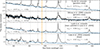 |
Fig. 10. Euclid Q1 geometric mean composite and three literature quasar composites, with NIR continua fitted with broken power laws over 0.75–1.35 μm. From top to bottom, the panels show the Euclid Q1 composite (geometric mean), the geometric mean composite from Glikman et al. (2006), the mean Landt et al. composite as published by Euclid Collaboration: Lusso et al. (2024), and the type 1 AGN composite from Euclid Collaboration: Lusso et al. (2024). The black curves show the composite spectra, the dashed blue lines show the best-fitting broken power laws in Fλ, and the vertical dashed orange lines indicate the break wavelength of 980 nm. The annotated indices αλ, 1 (αν, 1) and αλ, 2 (αν, 2) are the corresponding spectral slopes in Fλ (Fν) blueward and redward of the break. Selected emission lines are labelled in the top panel for reference. |
For the Euclid Q1 composite, we obtain αλ, 1 = −0.97 and αλ, 2 = −0.73. The type 1 composite from Euclid Collaboration: Lusso et al. (2024) has similar slopes, αλ, 1 = −1.00 and αλ, 2 = −0.57, while the Glikman et al. (2006) geometric mean composite yields αλ, 1 = −1.25 and αλ, 2 = −0.68. The mean Landt et al. composite shows a rather steep blue segment with αλ, 1 = −2.28 over 0.75–0.98 μm, then turns over to a much flatter slope, αλ, 2 = −0.56, over 0.98–1.35 μm. In the Fλ representation, all four composites show a mild flattening of the NIR continuum toward longer wavelengths. For comparison with the literature, the corresponding αν values (computed via αν = −[αλ + 2]) are listed in parentheses in Fig. 10. Our Euclid composite has the flattest continuum in the NIR (with the smallest change of slopes at the break), while the Landt et al. mean composite exhibits the largest curvature (change of slopes). As shown by Landt et al. (2013), the NIR spectral energy distribution (SED) of AGNs affected by strong host galaxy light are much flatter than those of AGNs with low host contribution. The flatness of the NIR continuum of our Euclid composite is therefore most likely due to the host galaxy light contribution of the low-redshift AGNs.
The observed central wavelengths of selected emission lines (Table 3) were measured from the mean composite with spectral fitting using QSOFITMORE (Fu 2025). For broad emission lines, including Mg II, Hβ, Hα, O I, He I, Paδ, Paγ, and Paβ, we fitted a narrow Gaussian component (FWHM ≤ 1200 km s−1) and 2–3 broad Gaussian components (FWHM > 1200 km s−1) to each line profile, and report the central wavelengths of the narrow components. For narrow (forbidden) lines, including [O II], [Ne III], [O III], and [S III], we fitted only one narrow component to each profile. The uncertainties are the standard deviations of a Monte Carlo simulation of 50 fits. As shown in Table 3, the line centres of narrow lines typically show lower uncertainties than those of the broad lines ([O III] λ5008 has the lowest wavelength uncertainty), indicating the significance of narrow lines in redshift determination.
Major emission lines identified from the mean composite quasar spectrum.
5. Discussion
5.1. Morphological properties of the bright quasar sample
With a pixel scale of  and stable PSF of VIS imaging, Euclid resolves obvious galaxy structure from the local Universe to at least z = 1.5 (with particularly rich statistics at 0.3 < z < 0.7; see e.g. Euclid Collaboration: Walmsley et al. 2026). These data enable the detailed structural characterisation of quasar hosts through uniform measurements of Sérsic-based and model-independent parameters (Euclid Collaboration: Quilley et al. 2026; Euclid Collaboration: Romelli et al. 2026), as well as the separation of compact nuclear light from extended galaxy emission (Euclid Collaboration: Margalef-Bentabol et al. 2026).
To take advantage of the detailed structural information provided by the VIS images, we examined two redshift regimes separately: (i) a low-redshift (z < 0.5) subset with 341 sources, and (ii) an intermediate-redshift (0.5 < z < 2) subset with 2361 sources. Both subsets are selected to have valid morphological parameters measured from VIS imaging, including parameters from the single-component Sérsic fit (Euclid Collaboration: Quilley et al. 2026): Sérsic index (nVIS), effective radius (Re,VIS), and axis ratio (ρVIS); and the model-independent CAS parameters (Conselice 2003; Euclid Collaboration: Romelli et al. 2026): concentration, asymmetry, and clumpiness (smoothness). The intermediate-redshift subset is further supplemented with a VIS PSF fraction (fPSF), derived by the deep-learning-based fPSF prediction model trained on simulated galaxy images with different levels of fPSF added to them (Euclid Collaboration: Margalef-Bentabol et al. 2026). We choose the redshift range 0.5 < z < 2 because the model was trained and validated in this range.
As shown in Fig. 11 and Table 4, the low-redshift population shows a large source extent with median μmax − mag = −1.67, significantly higher than the median μmax − mag = −2.87 of the intermediate-redshift sample. The μmax − mag value anticorrelates with the Sérsic index and concentration. In particular, the most compact sources in this population (μmax − mag ≈ −2.5) have a Sérsic index around 5.5, which is the upper limit set by Euclid Collaboration: Quilley et al. (2026). They have suggested that fits with Sérsic indices above 5.45 should be removed from any Sérsic-based analysis. In this low-redshift population, 50% of the sources have nVIS higher than 5.45. Such near-boundary Sérsic indices indicate that the single-component Sérsic model cannot describe the light profiles of AGNs with bright cores. When requiring nVIS < 5.45, the median nVIS is 2.31, which is still significantly higher than the peak value of 0.8 among all galaxies in Euclid Collaboration: Quilley et al. (2026). The median Re,VIS of nVIS < 5.45 sources is  , identical to the peak value of Re,VIS in Euclid Collaboration: Quilley et al. (2026).
 |
Fig. 11. Corner plot showing the joint distributions of morphological parameters measured from Euclid VIS imaging for 341 sources at z < 0.5. Displayed parameters include visual-inspection redshift (zvi), Sérsic index (nVIS), axis ratio (ρVIS), logarithmic effective radius (log10(Re,VIS/1″)), concentration (C), asymmetry (A), clumpiness (S), and μmax − mag. |
Median VIS morphology parameters and fPSF.
The CAS parameters further characterise the resolved structure of the low-redshift quasars. The median concentration (C = 4.27) is high compared to the general galaxy population (e.g. C ≈ 2.5, see Euclid Collaboration: Quilley et al. 2026) but with significant scatter, reflecting the coexistence of bright nuclear light and extended hosts. Asymmetry values are moderate (median A = 0.36) with a tail to A > 1, indicating disturbed morphologies or nearby companions. The clumpiness parameter is elevated (median S = 0.19), suggesting clumpy emission in many cases, possibly due to ongoing star formation (e.g. Conselice 2003, 2014). Overall, at z < 0.5, the host galaxies of bright quasars are frequently resolved and often display interacting features and star-forming clumps.
Compared to the low-redshift subset, the intermediate-redshift quasars at 0.5 < z < 2 are markedly more compact (see Fig. 12 and Table 4). More than 90% of the sources (2031) have near-boundary Sérsic indices of nVIS > 5.45, which results in a median nVIS = 5.5 and a median  (1/10 of the VIS pixel size). Such a high fraction of saturated Sérsic fits indicates that the single-component Sérsic model cannot capture the unresolved nuclear dominance of these sources. When restricting to nVIS < 5.45, the median Sérsic index decreases to 2.25 and the median effective radius increases to
  , values more consistent with resolved galaxy light profiles.
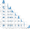 |
Fig. 12. Same as Fig. 11, but for 2361 sources at 0.5 < z < 2 with measurements of AGN PSF contribution fraction (fPSF). |
The VIS PSF fraction (fPSF) provides a more direct handle on this unresolved light. Its distribution peaks around 0.8 with another weaker peak around 0.1 (Fig. 12), confirming that most sources are dominated by their cores, consistent with their Sérsic fits converging to extreme values. Sources with high fPSF values also correspond to the most point-like objects, characterised by μmax − mag ≈ −2.9. However, low fPSF values (e.g. fPSF < 0.1) do not necessarily imply the absence of AGN activity, because uncertainties of the measurements could dominate at such low levels.
As shown in Fig. 12 and Table 4, the CAS parameters of the intermediate-redshift quasars show very different distributions compared to those of the low-redshift quasars. Highly left-skewed distributions of concentration (median C = 2.56) and clumpiness (median S = 0.08) are seen in intermediate-redshift quasars, in contrast to the nearly symmetric distributions of the two parameters for the low-redshift quasars (median C = 4.27 and median S = 0.19). The concentration and clumpiness distributions of the intermediate-redshift quasars appear unphysical, because quasar hosts are expected to be more concentrated and clumpier towards higher redshift. This discrepancy likely arises because the nuclear PSF components were not removed before the measurements. Indeed, sources with low nuclear fractions (fPSF ≲ 0.3) show more realistic Sérsic indices and CAS parameters, reinforcing that uncorrected nuclear light biases the structural measurements of the host galaxies.
Taken together, these results demonstrate that VIS morphology captures a strong redshift dependence in the apparent structure of bright quasars: (i) at z < 0.5, obvious host galaxy structures are frequently resolved, and a single Sérsic model can describe the light profiles of half of the sources; (ii) at 0.5 < z < 2, the nuclear component dominates, driving Sérsic indices of 90% of the sources to their upper limits. In this regime (0.5 < z < 2), fPSF offers a more reliable compactness measure and light profile characterisation than the single Sérsic fits, allowing us to quantify the balance between nuclear and host emission across the bright quasar sample. Representative Euclid 1D spectra and VIS cutouts illustrating these trends are shown in Appendix D for low-redshift sources (z < 0.5; Fig. D.1) and for 0.5 < z < 2 quasars spanning different fPSF levels (Fig. D.2). A more detailed analysis of AGN host galaxy morphology, including re-measurement of morphological parameters with methods tailored to AGN host galaxies, and dedicated tests to quantify measurement sensitivity as a function of host galaxy surface brightness, redshift, and nucleus-to-host contrast, will be presented in a follow-up study.
5.2. Euclid colour space, multi-wavelength selection, and future improvements
The advent of Euclid’s high-quality, wide-area near-infrared photometry opens a novel colour space for quasar selection, providing new opportunities to discover dust-reddened or intrinsically red quasars that are missed by traditional optical or ultraviolet (UV) selection. The extended wavelength coverage of the Euclid NIR bands, combined with precise VIS photometry, enables more robust discrimination of quasars from stars and galaxies, particularly at redshifts and extinction levels where classical techniques are less effective. Our initial exploration demonstrates that red quasars occupy distinct loci in Euclid colour-colour diagrams, highlighting the potential of the survey to identify populations that are heavily underrepresented in previous optical surveys.
Mid-infrared photometry from WISE has already proven highly effective for selecting luminous AGNs and quasars via their characteristic red MIR colours. Our analysis confirms that WISE-based colour cuts efficiently select AGN-dominated sources, as reflected in the properties of our pre-selected sample. However, WISE alone cannot distinguish between the most dust-obscured and less obscured quasars. The synergy between Euclid and WISE thus offers a powerful selection strategy: by combining WISE MIR colours with deep VIS and NIR photometry from Euclid, future quasar searches can achieve high completeness, efficiently probing obscured AGN populations.
Moreover, incorporating multi-band photometric data into the spectroscopic identification process will substantially improve the completeness and reliability of the quasar sample. Photometric pre-selection not only increases the likelihood of identifying genuine quasars, especially those with atypical SEDs, but also enhances redshift determination by providing prior constraints and mitigating degeneracies in the spectral fitting. The inclusion of Euclid and external photometry will be essential for robust identification and breaking redshift degeneracies from only one emission line.
A limitation of the present work is that the initial sample relies on pre-selection using Gaia and WISE catalogues, which may miss quasars outside the colour selection windows or at the limits of the Gaia and WISE sensitivity. In future Euclid data releases, the construction of a more complete quasar sample will be enabled by combining traditional pre-selected candidates with new candidates identified from Euclid photometry and by the SPE pipeline. This composite approach, leveraging the full capability of the Euclid data, will allow for the recovery of quasars with a wider range of colours, luminosities, and host properties.
In addition, we note that measuring the intrinsic spectral properties of quasars requires careful treatment of the host galaxy contribution. As demonstrated in Sect. 5.1, even in AGN-dominated sources, the host can provide a significant fraction of the observed flux, especially in the VIS band. Correctly separating nuclear and host emission is challenging and may introduce additional uncertainties in line and continuum measurements. Future analyses will benefit from improved morphological decomposition and SED modelling to robustly isolate the quasar component and fully exploit Euclid’s spectrophotometric capabilities.
6. Conclusions
In this work, we have presented a large sample of 3468 bright quasars covering the redshift range of 0 < z ≲ 4.8 identified with red-grism spectroscopy of the first Euclid Quick Data Release, including 2686 sources with new spectroscopic identifications relative to existing public compilations. To ensure identification efficiency, we focused on a high-purity input quasar candidate sample of 9214 sources based on GDR3-QSOs (Quaia, CatNorth, and CatSouth) and the AllWISE R90 AGN table. Through a template matching process based on the Pearson correlation function and a visual inspection campaign, we labelled quasars and determine their spectroscopic redshifts. The success rate of the spectroscopic identification is 38%.
From the identified sample, we estimated an empirical spectroscopic depth of JE ≲ 21.5 and HE ≲ 21.3 at the sensitivity of the Wide Field Survey, beyond which the number of securely identified quasars declines sharply. Our investigation of the novel Euclid colour space demonstrates its power in uncovering redder, dust-obscured quasars that may be missed by traditional optical and MIR selections. The synergy between Euclid and WISE photometry promises even greater completeness and diversity in future quasar surveys.
We constructed the first Euclid composite spectrum of bright quasars, covering rest-frame NUV to NIR wavelengths and free from telluric absorption, providing a valuable benchmark for future spectral studies. The spectroscopic bright quasar catalogue of this work, and the composite quasar spectrum, will be available at CDS. In addition, the spectral properties of the quasars will be derived by multi-component fitting (Euclid Collaboration: Calhau et al. in preparation).
We characterised VIS morphologies using single-Sérsic and model-independent (CAS) parameters, supplemented by a deep-learning PSF fraction, fPSF. At low redshift (z < 0.5), obvious host structures are frequently resolved, and a single Sérsic model describes the light profiles of about half of the sources. At intermediate redshift (0.5 < z < 2), the nuclear component dominates, driving Sérsic indices of roughly 90% of the sources to the upper bound; in this regime fPSF provides a more reliable compactness measure and is used to quantify the balance between nuclear and host emission across the sample.
Finally, we discuss current limitations, including the pre-selection bias and the challenges of host-nucleus decomposition, and outline pathways for improvement with upcoming Euclid data releases and advanced selection methods. The results presented here demonstrate the capability of Euclid slitless spectroscopy in building large quasar samples and provide a basis for extending this approach to the wide-area AGN censuses enabled by forthcoming Euclid data releases.
Data availability
The full catalogue of the identified quasars Table B.1 and the composite spectra (Table 2) are available at the CDS via https://cdsarc.cds.unistra.fr/viz-bin/cat/J/A+A/711/A285
Acknowledgments
We thank the two anonymous referees for their constructive reports and helpful suggestions, which improved the clarity and quality of this paper. The Euclid Consortium acknowledges the European Space Agency and a number of agencies and institutes that have supported the development of Euclid, in particular the Agenzia Spaziale Italiana, the Austrian Forschungsförderungsgesellschaft funded through BMIMI, the Belgian Science Policy, the Canadian Euclid Consortium, the Deutsches Zentrum für Luft- und Raumfahrt, the DTU Space and the Niels Bohr Institute in Denmark, the French Centre National d’Etudes Spatiales, the Fundação para a Ciência e a Tecnologia, the Hungarian Academy of Sciences, the Ministerio de Ciencia, Innovación y Universidades, the National Aeronautics and Space Administration, the National Astronomical Observatory of Japan, the Netherlandse Onderzoekschool Voor Astronomie, the Norwegian Space Agency, the Research Council of Finland, the Romanian Space Agency, the State Secretariat for Education, Research, and Innovation (SERI) at the Swiss Space Office (SSO), and the United Kingdom Space Agency. A complete and detailed list is available on the Euclid web site (www.euclid-ec.org/consortium/community/). This work has made use of the Euclid Quick Release Q1 data from the Euclid mission of the European Space Agency (ESA), 2025, https://doi.org/10.57780/esa-2853f3b. This research makes use of ESA Datalabs (datalabs.esa.int), an initiative by ESA’s Data Science and Archives Division in the Science and Operations Department, Directorate of Science. This work has made use of data from the European Space Agency (ESA) mission Gaia (https://www.cosmos.esa.int/gaia), processed by the Gaia Data Processing and Analysis Consortium (DPAC, https://www.cosmos.esa.int/web/gaia/dpac/consortium). Funding for the DPAC has been provided by national institutions, in particular the institutions participating in the Gaia Multilateral Agreement. This publication makes use of data products from the Wide-field Infrared Survey Explorer, which is a joint project of the University of California, Los Angeles, and the Jet Propulsion Laboratory/California Institute of Technology, and NEOWISE, which is a project of the Jet Propulsion Laboratory/California Institute of Technology. WISE and NEOWISE are funded by the National Aeronautics and Space Administration. This publication makes use of data from the Hyper Suprime-Cam (HSC). This research used data obtained with the Dark Energy Spectroscopic Instrument (DESI). DESI construction and operations is managed by the Lawrence Berkeley National Laboratory. This material is based upon work supported by the U.S. Department of Energy, Office of Science, Office of High-Energy Physics, under Contract No. DE–AC02–05CH11231, and by the National Energy Research Scientific Computing Center, a DOE Office of Science User Facility under the same contract. Additional support for DESI was provided by the U.S. National Science Foundation (NSF), Division of Astronomical Sciences under Contract No. AST-0950945 to the NSF’s National Optical-Infrared Astronomy Research Laboratory; the Science and Technology Facilities Council of the United Kingdom; the Gordon and Betty Moore Foundation; the Heising-Simons Foundation; the French Alternative Energies and Atomic Energy Commission (CEA); the National Council of Humanities, Science and Technology of Mexico (CONAHCYT); the Ministry of Science and Innovation of Spain (MICINN), and by the DESI Member Institutions: www.desi.lbl.gov/collaborating-institutions. The DESI collaboration is honored to be permitted to conduct scientific research on I’oligam Du’ag (Kitt Peak), a mountain with particular significance to the Tohono O’odham Nation. Any opinions, findings, and conclusions or recommendations expressed in this material are those of the author(s) and do not necessarily reflect the views of the U.S. National Science Foundation, the U.S. Department of Energy, or any of the listed funding agencies. This research uses services or data provided by the SPectra Analysis and Retrievable Catalog Lab (SPARCL) and the Astro Data Lab, which are both part of the Community Science and Data Center (CSDC) program at NSF National Optical-Infrared Astronomy Research Laboratory. NOIRLab is operated by the Association of Universities for Research in Astronomy (AURA), Inc. under a cooperative agreement with the National Science Foundation. This research made use of hips2fits (https://alasky.cds.unistra.fr/hips-image-services/hips2fits), a service provided by CDS. YF is financed by the Dutch Research Council (NWO) grant number OCENW.XL21.XL21.025. KIC acknowledges funding from the Dutch Research Council (NWO) through the award of the Vici Grant VI.C.212.036. VA, JC and FR acknowledge the support from the INAF Large Grant “AGN & Euclid: a close entanglement” Ob. Fu. 01.05.23.01.14.
References
- Aihara, H., Arimoto, N., Armstrong, R., et al. 2018, PASJ, 70, S4 [NASA ADS] [Google Scholar]
- Alonso, D., Fabbian, G., Storey-Fisher, K., et al. 2023, JCAP, 11, 043 [Google Scholar]
- Assef, R. J., Stern, D., Noirot, G., et al. 2018, ApJS, 234, 23 [Google Scholar]
- Bagley, M. B., Finkelstein, S. L., Koekemoer, A. M., et al. 2023, ApJ, 946, L12 [NASA ADS] [CrossRef] [Google Scholar]
- Bañados, E., Le Brun, V., Belladitta, S., et al. 2025, MNRAS, 542, 1088 [Google Scholar]
- Bertin, E., Schefer, M., Apostolakos, N., et al. 2020, ASP Conf. Ser., 527, 461 [NASA ADS] [Google Scholar]
- Blanton, M. R., Bershady, M. A., Abolfathi, B., et al. 2017, AJ, 154, 28 [Google Scholar]
- Boroson, T. A., & Meyers, K. A. 1992, ApJ, 397, 442 [NASA ADS] [CrossRef] [Google Scholar]
- Brammer, G. 2019, Astrophysics Source Code Library [record ascl:1905.001] [Google Scholar]
- Carnerero, M. I., Raiteri, C. M., Rimoldini, L., et al. 2023, A&A, 674, A24 [NASA ADS] [CrossRef] [EDP Sciences] [Google Scholar]
- Chambers, K. C., Magnier, E. A., Metcalfe, N., et al. 2016, ArXiv e-prints [arXiv:1612.05560] [Google Scholar]
- Chaussidon, E., Yèche, C., Palanque-Delabrouille, N., et al. 2023, ApJ, 944, 107 [NASA ADS] [CrossRef] [Google Scholar]
- Cioni, M. R. L., Clementini, G., Girardi, L., et al. 2011, A&A, 527, A116 [CrossRef] [EDP Sciences] [Google Scholar]
- Conselice, C. J. 2003, ApJS, 147, 1 [NASA ADS] [CrossRef] [Google Scholar]
- Conselice, C. J. 2014, ARA&A, 52, 291 [CrossRef] [Google Scholar]
- Croom, S. M., Smith, R. J., Boyle, B. J., et al. 2004, MNRAS, 349, 1397 [NASA ADS] [CrossRef] [Google Scholar]
- De Angeli, F., Weiler, M., Montegriffo, P., et al. 2023, A&A, 674, A2 [NASA ADS] [CrossRef] [EDP Sciences] [Google Scholar]
- Delchambre, L., Bailer-Jones, C. A. L., Bellas-Velidis, I., et al. 2023, A&A, 674, A31 [NASA ADS] [CrossRef] [EDP Sciences] [Google Scholar]
- DESI Collaboration (Abdul-Karim, M., et al.) 2025, ArXiv e-prints [arXiv:2503.14745] [Google Scholar]
- Doyon, R., Willott, C. J., Hutchings, J. B., et al. 2023, PASP, 135, 098001 [NASA ADS] [CrossRef] [Google Scholar]
- Ducourant, C., Krone-Martins, A., Galluccio, L., et al. 2023, A&A, 674, A11 [NASA ADS] [CrossRef] [EDP Sciences] [Google Scholar]
- Edge, A., Sutherland, W., Kuijken, K., et al. 2013, Messenger, 154, 32 [Google Scholar]
- Emerson, J., McPherson, A., & Sutherland, W. 2006, Messenger, 126, 41 [Google Scholar]
- Estrada, N., Mercurio, A., Vulcani, B., et al. 2023, A&A, 671, A146 [NASA ADS] [CrossRef] [EDP Sciences] [Google Scholar]
- Estrada-Carpenter, V., Papovich, C., Momcheva, I., et al. 2019, ApJ, 870, 133 [NASA ADS] [CrossRef] [Google Scholar]
- Euclid Collaboration (Lusso, E., et al.) 2024, A&A, 685, A108 [NASA ADS] [CrossRef] [EDP Sciences] [Google Scholar]
- Euclid Collaboration (Cropper, M., et al.) 2025, A&A, 697, A2 [Google Scholar]
- Euclid Collaboration (Jahnke, K., et al.) 2025, A&A, 697, A3 [Google Scholar]
- Euclid Collaboration (Mellier, Y., et al.) 2025, A&A, 697, A1 [Google Scholar]
- Euclid Collaboration (Aussel, H., et al.) 2026, A&A, 711, A1 [Google Scholar]
- Euclid Collaboration (Copin, Y., et al.) 2026, A&A, 711, A6 [Google Scholar]
- Euclid Collaboration (Margalef-Bentabol, B., et al.) 2026, A&A, 711, A18 [Google Scholar]
- Euclid Collaboration (Matamoro Zatarain, T., et al.) 2026, A&A, 711, A20 [Google Scholar]
- Euclid Collaboration (Quilley, L., et al.) 2026, A&A, 711, A8 [Google Scholar]
- Euclid Collaboration (Romelli, E., et al.) 2026, A&A, 711, A4 [Google Scholar]
- Euclid Collaboration (Roster, W., et al.) 2026, A&A, 711, A16 [Google Scholar]
- Euclid Collaboration (Tarsitano, F., et al.) 2026, A&A, 711, A19 [Google Scholar]
- Euclid Collaboration (Walmsley, M., et al.) 2026, A&A, 711, A9 [Google Scholar]
- Euclid Quick Release Q1. 2025, https://doi.org/10.57780/esa-2853f3b [Google Scholar]
- Evans, I. N., Evans, J. D., Martínez-Galarza, J. R., et al. 2024, ApJS, 274, 22 [NASA ADS] [CrossRef] [Google Scholar]
- Fan, X., Bañados, E., & Simcoe, R. A. 2023, ARA&A, 61, 373 [NASA ADS] [CrossRef] [Google Scholar]
- Fitzpatrick, M. J., Olsen, K., Economou, F., et al. 2014, SPIE Conf. Ser., 9149, 91491T [Google Scholar]
- Flesch, E. W. 2023, Open J. Astrophys., 6, 49 [NASA ADS] [CrossRef] [Google Scholar]
- Fruchter, A. S., & Hook, R. N. 2002, PASP, 114, 144 [NASA ADS] [CrossRef] [Google Scholar]
- Fu, Y. 2025, https://doi.org/10.5281/zenodo.15571037 [Google Scholar]
- Fu, Y. 2026, https://doi.org/10.5281/zenodo.18642758 [Google Scholar]
- Fu, Y., Wu, X.-B., Yang, Q., et al. 2021, ApJS, 254, 6 [NASA ADS] [CrossRef] [Google Scholar]
- Fu, Y., Wu, X.-B., Li, Y., et al. 2024, ApJS, 271, 54 [NASA ADS] [CrossRef] [Google Scholar]
- Fu, Y., Wu, X.-B., Bouwens, R. J., et al. 2025, ApJS, 279, 54 [Google Scholar]
- Gaia Collaboration (Klioner, S. A., et al.) 2022, A&A, 667, A148 [NASA ADS] [CrossRef] [EDP Sciences] [Google Scholar]
- Gaia Collaboration (Vallenari, A., et al.) 2023a, A&A, 674, A1 [NASA ADS] [CrossRef] [EDP Sciences] [Google Scholar]
- Gaia Collaboration (Bailer-Jones, C. A. L., et al.) 2023b, A&A, 674, A41 [NASA ADS] [CrossRef] [EDP Sciences] [Google Scholar]
- Glikman, E., Helfand, D. J., & White, R. L. 2006, ApJ, 640, 579 [NASA ADS] [CrossRef] [Google Scholar]
- Gordon, K. 2024, J. Open Source Softw., 9, 7023 [NASA ADS] [CrossRef] [Google Scholar]
- Gordon, K. D., Clayton, G. C., Decleir, M., et al. 2023, ApJ, 950, 86 [CrossRef] [Google Scholar]
- Green, G. M. 2018, J. Open Source Softw., 3, 695 [Google Scholar]
- Hall, P. B., Anderson, S. F., Strauss, M. A., et al. 2002, ApJS, 141, 267 [NASA ADS] [CrossRef] [Google Scholar]
- International Organization for Standardization& International Commission on Illumination. 2019, ISO/CIE 11664-4:2019 Colorimetry– Part 4: CIE 1976 L*a*b* Colour Space, https://www.iso.org/standard/74166.html [Google Scholar]
- Jauzac, M., Jullo, E., Kneib, J.-P., et al. 2012, MNRAS, 426, 3369 [Google Scholar]
- Juneau, S., Jacques, A., Pothier, S., et al. 2025, ASP Conf. Ser., 541, 77 [Google Scholar]
- Koekemoer, A. M., Faber, S. M., Ferguson, H. C., et al. 2011, ApJS, 197, 36 [NASA ADS] [CrossRef] [Google Scholar]
- Kümmel, M., Walsh, J. R., Pirzkal, N., Kuntschner, H., & Pasquali, A. 2009, PASP, 121, 59 [CrossRef] [Google Scholar]
- Kümmel, M., Álvarez-Ayllón, A., Bertin, E., et al. 2022, ArXiv e-prints [arXiv:2212.02428] [Google Scholar]
- Landt, H., Bentz, M. C., Ward, M. J., et al. 2008, ApJS, 174, 282 [NASA ADS] [CrossRef] [Google Scholar]
- Landt, H., Elvis, M., Ward, M. J., et al. 2011, MNRAS, 414, 218 [NASA ADS] [CrossRef] [Google Scholar]
- Landt, H., Ward, M. J., Peterson, B. M., et al. 2013, MNRAS, 432, 113 [NASA ADS] [CrossRef] [Google Scholar]
- Leys, C., Ley, C., Klein, O., Bernard, P., & Licata, L. 2013, J. Exp. Social Psychol., 49, 764 [Google Scholar]
- Mainzer, A., Bauer, J., Grav, T., et al. 2011, ApJ, 731, 53 [Google Scholar]
- Marocco, F., Eisenhardt, P. R. M., Fowler, J. W., et al. 2021, ApJS, 253, 8 [Google Scholar]
- Mateos, S., Alonso-Herrero, A., Carrera, F. J., et al. 2012, MNRAS, 426, 3271 [Google Scholar]
- McMahon, R. G., Banerji, M., Gonzalez, E., et al. 2013, Messenger, 154, 35 [Google Scholar]
- Merloni, A., Lamer, G., Liu, T., et al. 2024, A&A, 682, A34 [NASA ADS] [CrossRef] [EDP Sciences] [Google Scholar]
- Meyer, R. A., Oesch, P. A., Giovinazzo, E., et al. 2024, MNRAS, 535, 1067 [CrossRef] [Google Scholar]
- Minniti, D., Lucas, P. W., Emerson, J. P., et al. 2010, New Astron., 15, 433 [Google Scholar]
- Miyazaki, S., Komiyama, Y., Kawanomoto, S., et al. 2018, PASJ, 70, S1 [NASA ADS] [Google Scholar]
- Momcheva, I. G., Brammer, G. B., van Dokkum, P. G., et al. 2016, ApJS, 225, 27 [Google Scholar]
- Myers, A. D., Outram, P. J., Shanks, T., et al. 2003, MNRAS, 342, 467 [Google Scholar]
- Myers, A. D., Palanque-Delabrouille, N., Prakash, A., et al. 2015, ApJS, 221, 27 [NASA ADS] [CrossRef] [Google Scholar]
- Navarro, V., del Rio, S., Angel Diego, M., et al. 2024, Space Data Management. Studies in Big Data, 141, 1 [Google Scholar]
- Neveux, R., Burtin, E., de Mattia, A., et al. 2020, MNRAS, 499, 210 [NASA ADS] [CrossRef] [Google Scholar]
- Nikutta, R., Fitzpatrick, M., Scott, A., & Weaver, B. A. 2020, Astron. Comput., 33, 100411 [Google Scholar]
- Oesch, P. A., Brammer, G., Naidu, R. P., et al. 2023, MNRAS, 525, 2864 [NASA ADS] [CrossRef] [Google Scholar]
- Oke, J. B., & Gunn, J. E. 1983, ApJ, 266, 713 [NASA ADS] [CrossRef] [Google Scholar]
- Onken, C. A., Wolf, C., Bessell, M. S., et al. 2024, PASA, 41, e061 [NASA ADS] [CrossRef] [Google Scholar]
- Osmer, P. S., & Hewett, P. C. 1991, ApJS, 75, 273 [Google Scholar]
- Petter, G. C., Hickox, R. C., Alexander, D. M., et al. 2023, ApJ, 946, 27 [NASA ADS] [CrossRef] [Google Scholar]
- Pirzkal, N., Xu, C., Malhotra, S., et al. 2004, ApJS, 154, 501 [Google Scholar]
- Planck Collaboration XLVIII. 2016, A&A, 596, A109 [NASA ADS] [CrossRef] [EDP Sciences] [Google Scholar]
- Pullen, A. R., Alam, S., & Ho, S. 2015, MNRAS, 449, 4326 [Google Scholar]
- Ricci, F., Treister, E., Bauer, F. E., et al. 2022, ApJS, 261, 8 [NASA ADS] [CrossRef] [Google Scholar]
- Richards, G. T., Fan, X., Newberg, H. J., et al. 2002, AJ, 123, 2945 [NASA ADS] [CrossRef] [Google Scholar]
- Rieke, M. J., Kelly, D., & Horner, S. 2005, SPIE Conf. Ser., 5904, 1 [NASA ADS] [Google Scholar]
- Rieke, M. J., Kelly, D. M., Misselt, K., et al. 2023, PASP, 135, 028001 [CrossRef] [Google Scholar]
- Rimoldini, L., Holl, B., Gavras, P., et al. 2023, A&A, 674, A14 [NASA ADS] [CrossRef] [EDP Sciences] [Google Scholar]
- Roberts-Borsani, G., Morishita, T., Treu, T., et al. 2022, ApJ, 938, L13 [NASA ADS] [CrossRef] [Google Scholar]
- Sartoretti, P., Katz, D., Cropper, M., et al. 2018, A&A, 616, A6 [NASA ADS] [CrossRef] [EDP Sciences] [Google Scholar]
- Schlafly, E. F., Meisner, A. M., & Green, G. M. 2019, ApJS, 240, 30 [Google Scholar]
- Schmidt, M., Schneider, D. P., & Gunn, J. E. 1986, ApJ, 306, 411 [Google Scholar]
- Schneider, D. P., Schmidt, M., & Gunn, J. E. 1999, AJ, 117, 40 [Google Scholar]
- Sharon, K., Cerny, C., Rigby, J. R., et al. 2022, ArXiv e-prints [arXiv:2207.05709] [Google Scholar]
- Simcoe, R. A., Burgasser, A. J., Bernstein, R. A., et al. 2008, SPIE Conf. Ser., 7014, 70140U [NASA ADS] [Google Scholar]
- Stern, D., Assef, R. J., Benford, D. J., et al. 2012, ApJ, 753, 30 [Google Scholar]
- Storey-Fisher, K., Hogg, D. W., Rix, H.-W., et al. 2024, ApJ, 964, 69 [NASA ADS] [CrossRef] [Google Scholar]
- Sun, F., Egami, E., Pirzkal, N., et al. 2023, ApJ, 953, 53 [NASA ADS] [CrossRef] [Google Scholar]
- Urrutia, T., Becker, R. H., White, R. L., et al. 2009, ApJ, 698, 1095 [Google Scholar]
- Vanden Berk, D. E., Richards, G. T., Bauer, A., et al. 2001, AJ, 122, 549 [Google Scholar]
- Webb, N. A., Coriat, M., Traulsen, I., et al. 2020, A&A, 641, A136 [NASA ADS] [CrossRef] [EDP Sciences] [Google Scholar]
- Williams, C. C., Tacchella, S., Maseda, M. V., et al. 2023, ApJS, 268, 64 [NASA ADS] [CrossRef] [Google Scholar]
- Willott, C. J., Doyon, R., Albert, L., et al. 2022, PASP, 134, 025002 [CrossRef] [Google Scholar]
- Wright, E. L., Eisenhardt, P. R. M., Mainzer, A. K., et al. 2010, AJ, 140, 1868 [Google Scholar]
- Wu, X.-B., Hao, G., Jia, Z., Zhang, Y., & Peng, N. 2012, AJ, 144, 49 [Google Scholar]
Appendix A: Sources with initially discrepant redshifts in the DESI comparison
We illustrate the 16 initially discrepant sources in the DESI consistency check, defined as |zvi−zDESI|/(1 + zDESI) > 0.15 among the 454 quasars in common between our Q1 sample and DESI DR1. For each of the 16 sources, we retrieve the DESI DR1 coadded 1D spectrum and the corresponding redshift (zDESI) from the DESI redshift catalogue using the SPectra Analysis and Retrievable Catalog Lab (SPARCL; Juneau et al. 2025) and the Astro Data Lab (Fitzpatrick et al. 2014; Nikutta et al. 2020), and compare them to the Euclid RGE spectrum used in our visual inspection. The assessment focuses on whether the main emission features are mutually consistent between the DESI and Euclid spectra at the proposed redshift solution.
Figure A.1 shows the DESI and Euclid spectra together with the template spectrum evaluated at the final zvi. For 11 sources, both DESI and Euclid spectra support our visual redshift solution, and zDESI is inconsistent with the spectra. For the remaining five sources whose visual redshifts are revised after reinspection, the panel titles list the updated zvi together with the initial (incorrect) zvi in parentheses; the updated values are adopted in the final catalogue.
 |
Fig. A.1. DESI (blue) and Euclid (green) spectra for the 16 objects that initially satisfy |zvi−zDESI|/(1 + zDESI) > 0.15 among the 454 quasars in common with DESI DR1. The dashed red curve shows the quasar template spectrum evaluated at the final zvi (scaled for display). Vertical dotted lines mark the expected observed wavelengths of common quasar emission lines at the final zvi. Panels outlined in orange denote the five sources for which we revise zvi after reinspection; for these, the initial (incorrect) zvi is reported in parentheses after the updated zvi in the panel title. |
As shown in Fig. A.1, most of the 11 sources for which zDESI is inconsistent with the spectra exhibit an unusually red rest-frame UV continuum. In addition, several of these objects (Euclid Q1 object_id: 2663629828654232723, 2671669943665629138, 2725249569662970807, 2695896801645034348, and 2718727659662564020) show broad absorption troughs, including absorption associated with Mg II and other metal transitions, consistent with the unusual low-ionisation broad absorption line (LoBAL; see e.g. Boroson & Meyers 1992; Hall et al. 2002; Urrutia et al. 2009) quasars. Because such strongly reddened and LoBAL quasars are relatively rare in the training and template sets used by automated pipelines, and because their red, observed-frame optical continua often have lower S/N than those of typical blue quasars, automated redshift measurements can be less reliable for these objects.
For the remaining five sources, the main causes of the initial misidentifications of zvi are (i) line-identification degeneracies when only a single prominent feature is present, and (ii) artefacts that complicate the interpretation of the spectrum. In particular, in two cases (object_id: 2689353840663761572, and 2680117565652270034) an emission feature consistent with H α at the correct redshift was initially misidentified as Mg II, leading to spuriously high redshift estimates (zvi > 4). In another case (object_id: 2664764876670636991), an emission feature consistent with H β at the correct redshift was initially interpreted as H α, leading to an overestimated redshift. Conversely, for object 2675695970669312051, H α was initially misidentified as H β, leading to an underestimated redshift. Finally, for object 2667540229671259497, the Euclid spectrum is strongly affected by artefacts (anomalous spike and bump), likely related to contamination from a nearby source, and the initial redshift estimate was driven by the spike seen in the Euclid spectrum.
Appendix B: Description of the spectroscopically identified bright quasar catalogue
The format of the catalogue of spectroscopically identified bright quasars from Euclid Q1 is shown in Table B.1. The full catalogue will be available at https://cdsarc.cds.unistra.fr/.
Format of the catalogue of spectroscopically identified bright quasars from Euclid Q1.
Appendix C: Composite spectra generation with 1D drizzle
C.1. Details of the 1D drizzle method
We construct Euclid quasar composite spectra on a common rest-frame grid with a constant bin size of Δλ = 4 Å. The mapping preserves the integrated flux density in each bin through a linear, flux-conserving rebinning that partitions every input pixel across the overlapping output bins in proportion to the fractional overlap in wavelength. This procedure is mathematically equivalent to a one-dimensional version of the Drizzle algorithm (Fruchter & Hook 2002) and matches the smallest native rest-frame pixel size at the blue end of our spectra, while mildly oversampling the data at longer wavelengths.
Preprocessing and normalisation. Each spectrum is shifted to the rest frame using the adopted redshift, then converted to rest-frame flux density in Fλ via Fλ, rest = (1 + z) Fλ, obs. The spectra are rebinned onto the common rest-frame grid with the flux-conserving drizzle scheme described below. Each rebinned spectrum is then normalised to the running composite within the spectral overlap so that relative shapes are combined consistently; the same normalisation factor is applied to the spectrum’s per-pixel variances. We ignore pixels with non-finite or non-positive flux or variance values.
The 1D drizzle rebinning and variance propagation. Let fp and  be the flux and variance in input pixel p, whose wavelength interval is [λp − 1/2, λp + 1/2] with width Δλp = λp + 1/2 − λp − 1/2. The j-th output bin covers [λj − 1/2, λj + 1/2] with width Δλj. We define the fractional overlap
![Mathematical equation: $$ \begin{aligned} A_{jp} = \frac{\max \bigl (0,\,\min [\lambda _{p+1/2},\lambda _{j+1/2}] - \max [\lambda _{p-1/2},\lambda _{j-1/2}]\bigr )}{\Delta \lambda _{p}}\,, \end{aligned} $$](/articles/aa/full_html/2026/07/aa58490-25/aa58490-25-eq19.gif) (C.1)
(C.1)
so that 0 ≤ Ajp ≤ 1 and ∑jAjp = 1 for fully covered pixels. The rebinned flux and variance for a single spectrum in bin j are then
 (C.2)
(C.2)
 (C.3)
(C.3)
assuming uncorrelated input pixels. This operation introduces correlations between neighbouring output bins, but it preserves total flux and provides a well-defined per-bin variance. In the following, we treat  as the effective per-bin uncertainty and note the presence of correlations where relevant.
Equal-weight mean and its uncertainty. For the mean composite we combine, in each bin j, all rebinned spectra that have valid data in that bin with equal weights. If nj spectra contribute and their rebinned fluxes and variances are  and
and  , the mean composite and its formal uncertainty are
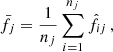 (C.4)
(C.4)
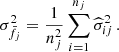 (C.5)
(C.5)
In the implementation we apply sigma clipping in each wavelength bin to reduce the impact of outliers before computing the mean. The sigma-clipping is performed using astropy.stats.sigma_clip, with a threshold of sigma=6, and a robust standard deviation estimator calculated as
 (C.6)
(C.6)
where MAD is the median absolute deviation (Leys et al. 2013). For a univariate dataset X1, X2, ..., Xn, the MAD is defined as the median of the absolute deviations from the data’s median
 (C.7)
(C.7)
In addition, we track the observed object-to-object dispersion in each bin after sigma-clipping via the central second moment
 (C.8)
(C.8)
whose square root is stored as the ‘RMS’ spectrum. This sj includes both intrinsic diversity and measurement noise and is quoted separately from the statistical uncertainty  on the mean.
Median composite. We formed a median composite by taking, in each bin, the median of the contributing  values. We applied the same sigma clipping as done when computing the mean composite. We did not attach formal uncertainties to the median composite.
Geometric-mean composite for continuum shape. To preserve the average continuum slope of quasars, we also computed a geometric-mean composite on the same rebinned spectra and wavelength grid, again using equal weights. For contributors with positive flux,
 (C.9)
(C.9)
 (C.10)
Using error propagation for  with
with ![Mathematical equation: $ \mathrm{Var}[\ln \hat f_{ij}] \approx \widehat{\sigma}_{ij}^{2}/\hat f_{ij}^{2} $](/articles/aa/full_html/2026/07/aa58490-25/aa58490-25-eq35.gif) when
when  , the uncertainty on μj and the geometric-mean flux are
 (C.11)
 (C.12)
We masked bins where fewer than three spectra contribute or where negative flux values prevent a robust logarithmic mean from being determined.
Effect of wavelength bin size. In Sect. 4.3 we adopted a bin size of Δλ = 4 Å for constructing the Euclid mean composite spectrum. To assess the impact of this choice, we recomputed the mean composite using coarser grids with Δλ = 8 Å and 13.4 Å, keeping all other steps of the stacking procedure fixed. As shown in Fig. C.1, the continuum shapes of three mean composites are virtually identical in both the optical and near-infrared ranges, while the two larger bin sizes produce undersampled, flattened emission line peaks. This test demonstrates that the bin size of Δλ = 4 Å is favourable for the preservation of details of the composite spectra.
 |
Fig. C.1. Mean Euclid Q1 quasar composite spectra constructed with different rest-frame wavelength bin sizes. The three curves show mean composites built on grids with Δλ = 4.0 Å (blue), 8.0 Å (orange), and 13.4 Å (green). For clarity, the spectra are vertically offset by multiplicative factors, as indicated on the right-hand side. The top panel displays the optical range (300–700 nm) and the bottom panel shows the near-infrared range (700–1400 nm). The continua of the three spectra show close agreement, while the two spectra with larger bin sizes have flattened emission line peaks. |
C.2. Construction of the piecewise quasar template
The final rest-frame template combines
-
Vanden Berk et al. (2001) for λrest < 320 nm;
-
The mean composite from this work for 320 ≤ λrest ≤ 1550 nm; and
-
Glikman et al. (2006) for λrest > 1550 nm.
All three spectra are resampled onto a common rest-frame grid from 90 to 2100 nm with a spacing of 0.2 nm using a flux-conserving resampler (specutils.FluxConservingResampler). Before splicing, we scale the adjoining segments using the mean flux in 5 nm windows centred on each join. At 320 nm we scale our composite to match Vanden Berk et al. (2001); at 1550 nm we scale Glikman et al. (2006) to match our composite. If ⟨FA⟩ and ⟨FB⟩ are the mean fluxes in the overlap window, the scale factor applied to FB is s = ⟨FA⟩/⟨FB⟩. After scaling, we combine the spectra piecewise at the join wavelengths (no additional cross-fade). The resulting template covers 90 to 2100 nm on a uniform grid.
Appendix D: Example cutouts of quasars
We present the Euclid spectra and image cutouts of a sample of low-redshift (z < 0.5) quasars in Fig. D.1, and a sample of intermediate-redshift (0.5 < z < 2) quasars in Fig. D.2.
 |
Fig. D.1. Euclid 1D spectra and imaging cutouts for a random sample of 10 low-redshift (z < 0.5) sources. Each panel displays the 1D spectrum (top) and five imaging cutouts with 10″ sizes (bottom) in the IE, YE, JE, and HE bands, as well as a VIS-YE composite. The composite image is generated by mapping the VIS and YE fluxes into the blue and red channels, respectively, with their mean used for green, and the VIS band used to define overall luminosity in the L*a*b* colour space (International Organization for Standardization & International Commission on Illumination 2019) to enhance morphological detail. Major emission lines detected in the wavelength range [12 047, 18 734] Å are marked. |
 |
Fig. D.2. Same as Fig. D.1, but for 10 intermediate-redshift (0.5 < z < 2) quasars with different fPSF levels. |
All Tables
Mean, geometric mean, and median Euclid Q1 quasar composite spectra, along with RMS, S/N and the number of spectra in each wavelength bin (Nspec).
Format of the catalogue of spectroscopically identified bright quasars from Euclid Q1.
All Figures
|
Fig. 1. Example Euclid spectra of the visually identified quasars in the rest frame. The four columns from left to right show prominent emission lines used for the visual inspection in descending order of redshift: Mg II in the first column; H β, [O III], and H γ in the second column; H α in the third column; and He I + Pa γ, Pa β, Pa δ, and [S III] in the last column. |
| In the text | |
|
Fig. 2. Concentration parameter μmax − mag as a function of the visual redshift zvi. The rejected region is shaded in pink, and is defined with μmax − mag > −2 at zvi > 2, as indicated by the dashed red lines. Sources inside the rejected region are considered to have spurious redshifts and are marked with black crosses. |
| In the text | |
|
Fig. 3. Redshift-magnitude distributions for the visually identified quasar sample using Euclid Q1 data. Top: Two-dimensional distribution of HE versus zvi. Gaia-detected sources are shown as blue open squares, and sources not in Gaia DR3 are shown as orange circles. Blue contours trace the density of the Gaia subset, and red contours trace the density of the non-Gaia subset. The marginal histograms for zvi (above) and HE (right) show the full sample (black steps), the Gaia subset (blue steps), and the non-Gaia subset (orange steps). Bottom: One-dimensional histograms of IE, YE, and JE for the same three samples. All histograms are normalised to unit area. |
| In the text | |
|
Fig. 4. Left: Distribution of the median spectral S/N within [12 047, 18 734] Å for visually identified quasars. The dashed red line at S/N = 2 marks an empirical threshold below which the number of successful identifications declines rapidly. Middle and right: Median S/N versus JE and HE magnitudes, respectively. Blue points show individual quasars, and the black lines indicate linear fits to log10(S/N), with the fitted relations annotated. The dashed red line again marks S/N = 2, and its intersection with the fit defines empirical limiting magnitudes of JE ≈ 21.5 and HE ≈ 21.3, shown by dashed green lines. These values represent practical limits for reliable spectral identification of quasars in Q1. |
| In the text | |
|
Fig. 5. W1 − W2 versus W2 − W3 colour-colour diagram of spectroscopically identified quasars in this work, where Gaia-detected sources are shown as blue open squares, and sources not in Gaia DR3 are shown as orange circles. The density distribution of the full identified quasar sample is indicated with green contour lines. Euclid point-like sources are shown as grey triangles. To ensure the reliability of the colours, only sources with adequate S/N (w1snr > 5, w2snr > 5, and w3snr > 3) are shown. |
| In the text | |
|
Fig. 6. Euclid and external (Hyper Suprime-Cam, HSC; Miyazaki et al. 2018; Aihara et al. 2018) colour-colour diagrams of spectroscopically identified quasars in this work, where Gaia-detected sources are shown as blue open squares, and sources not in Gaia DR3 are shown as orange circles. The density distribution of the Gaia-detected sample is indicated with blue contour lines, and that of the non-Gaia sample is indicated with red contour lines. The density of Euclid point-like sources is shown as grey hexagonal binning plots in the background. |
| In the text | |
|
Fig. 7. Stacked emission-line map of the golden sample of 2868 visually identified quasars. Each row of the pixels represents a spectrum normalised using its 25th and 95th percentiles. Prominent emission lines are marked with text labels. |
| In the text | |
|
Fig. 8. Mean and median composite quasar spectra constructed from our golden sample (black and red curves, respectively), with the RMS scatter around the mean composite indicated by the shaded blue region. The quasar composite spectrum from Glikman et al. (2006) is plotted in magenta, the type 1 AGN composite from Euclid Collaboration: Lusso et al. (2024) is plotted in green, and the mean composite constructed using data from Landt et al. (2008, 2011, 2013) is plotted in orange. Prominent emission lines are marked for reference. |
| In the text | |
|
Fig. 9. Diagnostics of the Euclid Q1 mean quasar composite as a function of rest-frame wavelength for a bin size of Δλ = 4 Å. Top: number of spectra contributing to each wavelength bin. Middle: S/N of the mean composite per bin. Bottom: RMS dispersion of the contributing spectra about the mean. Vertical dashed lines mark the rest wavelengths of prominent emission lines, which are labelled in the top panel. |
| In the text | |
|
Fig. 10. Euclid Q1 geometric mean composite and three literature quasar composites, with NIR continua fitted with broken power laws over 0.75–1.35 μm. From top to bottom, the panels show the Euclid Q1 composite (geometric mean), the geometric mean composite from Glikman et al. (2006), the mean Landt et al. composite as published by Euclid Collaboration: Lusso et al. (2024), and the type 1 AGN composite from Euclid Collaboration: Lusso et al. (2024). The black curves show the composite spectra, the dashed blue lines show the best-fitting broken power laws in Fλ, and the vertical dashed orange lines indicate the break wavelength of 980 nm. The annotated indices αλ, 1 (αν, 1) and αλ, 2 (αν, 2) are the corresponding spectral slopes in Fλ (Fν) blueward and redward of the break. Selected emission lines are labelled in the top panel for reference. |
| In the text | |
|
Fig. 11. Corner plot showing the joint distributions of morphological parameters measured from Euclid VIS imaging for 341 sources at z < 0.5. Displayed parameters include visual-inspection redshift (zvi), Sérsic index (nVIS), axis ratio (ρVIS), logarithmic effective radius (log10(Re,VIS/1″)), concentration (C), asymmetry (A), clumpiness (S), and μmax − mag. |
| In the text | |
|
Fig. 12. Same as Fig. 11, but for 2361 sources at 0.5 < z < 2 with measurements of AGN PSF contribution fraction (fPSF). |
| In the text | |
|
Fig. A.1. DESI (blue) and Euclid (green) spectra for the 16 objects that initially satisfy |zvi−zDESI|/(1 + zDESI) > 0.15 among the 454 quasars in common with DESI DR1. The dashed red curve shows the quasar template spectrum evaluated at the final zvi (scaled for display). Vertical dotted lines mark the expected observed wavelengths of common quasar emission lines at the final zvi. Panels outlined in orange denote the five sources for which we revise zvi after reinspection; for these, the initial (incorrect) zvi is reported in parentheses after the updated zvi in the panel title. |
| In the text | |
|
Fig. C.1. Mean Euclid Q1 quasar composite spectra constructed with different rest-frame wavelength bin sizes. The three curves show mean composites built on grids with Δλ = 4.0 Å (blue), 8.0 Å (orange), and 13.4 Å (green). For clarity, the spectra are vertically offset by multiplicative factors, as indicated on the right-hand side. The top panel displays the optical range (300–700 nm) and the bottom panel shows the near-infrared range (700–1400 nm). The continua of the three spectra show close agreement, while the two spectra with larger bin sizes have flattened emission line peaks. |
| In the text | |
|
Fig. D.1. Euclid 1D spectra and imaging cutouts for a random sample of 10 low-redshift (z < 0.5) sources. Each panel displays the 1D spectrum (top) and five imaging cutouts with 10″ sizes (bottom) in the IE, YE, JE, and HE bands, as well as a VIS-YE composite. The composite image is generated by mapping the VIS and YE fluxes into the blue and red channels, respectively, with their mean used for green, and the VIS band used to define overall luminosity in the L*a*b* colour space (International Organization for Standardization & International Commission on Illumination 2019) to enhance morphological detail. Major emission lines detected in the wavelength range [12 047, 18 734] Å are marked. |
| In the text | |
|
Fig. D.2. Same as Fig. D.1, but for 10 intermediate-redshift (0.5 < z < 2) quasars with different fPSF levels. |
| In the text | |
Current usage metrics show cumulative count of Article Views (full-text article views including HTML views, PDF and ePub downloads, according to the available data) and Abstracts Views on Vision4Press platform.
Data correspond to usage on the plateform after 2015. The current usage metrics is available 48-96 hours after online publication and is updated daily on week days.
Initial download of the metrics may take a while.