


| Issue |
A&A
Volume 710, June 2026
|
|
|---|---|---|
| Article Number | A250 | |
| Number of page(s) | 10 | |
| Section | The Sun and the Heliosphere | |
| DOI | https://doi.org/10.1051/0004-6361/202660162 | |
| Published online | 17 June 2026 | |
Statistical analysis of solar energetic particle rise times using Earth and Mars observations and constraints on particle transport parameters
1
Deep Space Exploration Laboratory/School of Earth and Space Sciences, University of Science and Technology of China, Hefei, PR China
2
Institute of Modern Physics, Chinese Academy of Sciences, Lanzhou, China
3
National Key Laboratory of Space Environment Interaction with Matters, Lanzhou Institute of Physics, Lanzhou, China
★ Corresponding author: This email address is being protected from spambots. You need JavaScript enabled to view it.
Received:
31
March
2026
Accepted:
25
April
2026
Abstract
Context. The propagation of solar energetic particles (SEPs) in interplanetary space is modulated by turbulence caused by the solar wind, which significantly affects the particle diffusion and energy evolution through scattering processes. However, traditional analyses based on absolute flux measurements face inherent difficulties in separating the effects of particle acceleration at the source from subsequent transport processes. In contrast, the temporal features of SEPs, such as the onset and peak times, are less affected by these uncertainties and are therefore more suitable for exploring the transport process of SEPs.
Aims. We establish a statistical relation between the rise time of SEP events at different energies using multi-satellite observations at Earth and Mars. The results are used to further invert the turbulence parameters affecting the transport of SEPs based on a parallel diffusion model, thereby revealing the characteristics and evolutionary trend of turbulence at different radial distances.
Methods. Using data from SOHO/ERNE and Tianwen-1/MEPA between November 2020 and March 2025, we selected 75 SEP events at 1 AU and 58 events near Mars. For each energy range of each event, the onset time was determined by a linear fitting method, and the peak time was extracted using a sliding median filter combined with Savitzky-Golay smoothing methods. The difference between the onset time and the peak time subsequently determines the SEP rise time. Together with the theoretical relation of rise time and its dependence on energy derived from the pure diffusion equation, we compared the statistical behavior of the rise time between Earth and Mars.
Results. Despite uncertainties introduced by the selection criteria of SEP events, the rise time of SEP events, Δt in minutes, follows a clear power-law relation with energy (Δt ∝ Eη), with η = −0.368 ± 0.058 averaged for SEP events near Earth and η = −0.302 ± 0.031 averaged for events near Mars. The flatter power-law shape at Mars suggests that the dependence of the rise time on energy weakens with increasing radial distance from the Sun. Based on these empirical relations, we constrain the rigidity dependence of the parallel mean free path of SEPs within the parallel diffusion model. Based on the simple assumption of a pure diffusion model, our results indicate that turbulence scattering of energetic particles at Mars approaches a rigidity-independent regime, reflecting an evolutionary trend of turbulence toward a dissipation-dominated state from Earth to Mars.
Key words: Sun: activity / Sun: particle emission
© The Authors 2026
 Open Access article, published by EDP Sciences, under the terms of the Creative Commons Attribution License (https://creativecommons.org/licenses/by/4.0), which permits unrestricted use, distribution, and reproduction in any medium, provided the original work is properly cited.
This article is published in open access under the Subscribe to Open model. This email address is being protected from spambots. You need JavaScript enabled to view it. to support open access publication.
1. Introduction
Solar energetic particle (SEP) events are energetic particle populations originating from solar eruption activities. They consist of protons, electrons, and heavy ions, with energies typically ranging from suprathermal (a few keV) to relativistic (a few GeV) (Desai & Giacalone 2016). Our current understanding of the spatial distribution and temporal evolution of SEPs has benefited significantly from recent multi-satellite observations (Guo et al. 2024). However, considerable uncertainties in flux measurements arise from instrument cross-calibration discrepancies, particle anisotropy, and contamination of low-energy channels by high-energy particle deposits (e.g., Lario et al. 2013; Li et al. 2020), which pose further challenges for quantitative studies of SEP transport. On the other hand, temporal parameters such as the onset and peak times of flux are less affected by these factors, making them more robust diagnostic parameters for a multi-satellite SEP event analysis (Meyer et al. 1956; Krucker & Lin 2000). Therefore, it is crucial to investigate how the rise times (time duration between onset and peak times) of SEP events vary with radial distance for understanding the transport mechanisms of particles in interplanetary space.
The analysis of the SEP rise time is grounded in the interpretation of the particle time-intensity profile, which includes the source injection and transport information. The theoretical study of SEP transport dates back to Meyer et al. (1956), who interpreted the time profile of the ground-level enhancement (GLE) events using the diffusion equation. This framework was later extended by Parker (1965) to the classic transport equation, which comprehensively describes particle motion under diffusion, adiabatic cooling, and magnetic focusing in the interplanetary magnetic field. This equation is typically solved numerically with assumed particle injection functions for comparison with observations because it is complex (e.g., Heras et al. 1992, 1995; Dröge 1994; Qin et al. 2006; Zhang et al. 2009; Hu et al. 2017; Whitman et al. 2023).
From an observational perspective, the SEP time-intensity profile is often described as a product of a power law and an exponential function (Farwa et al. 2025). Consequently, the Weibull distribution proposed by Wilks (2011) has been widely used to fit the observed time-intensity profiles. Subsequent studies, such as Kahler & Ling (2017), employed a modified Weibull function for the fitting, which has the general form
![Mathematical equation: $$ \begin{aligned} F(t) = \left|\frac{a}{b}\right|\left(\frac{t}{b}\right)^{a-1}\cdot \mathrm{exp}\left[-\left(\frac{t}{b}\right)^a\right]. \end{aligned} $$](/articles/aa/full_html/2026/06/aa60162-26/aa60162-26-eq1.gif) (1)
(1)
Here, F represents the intensity of SEPs, t is the time from event onset, the positive parameter a defines the profile shape, and b is the scaling parameter that stretches or compresses the basic shape of the event along the t-axis.
Laurenza et al. (2016) and Pallocchia et al. (2017) suggested that the Weibull distribution can serve as an asymptotic solution to the diffusion-loss equation, while Chiappetta et al. (2021) proposed a connection to stochastic acceleration mechanisms in turbulence. However, the shape parameter a and the scaling parameter b lack a clear physical correspondence in the Weibull distribution. This limits its utility for explaining specific physical processes.
Some studies have focused on simplified scenarios to isolate individual physical effects. Krimigis (1965) noted that under diffusion-dominated conditions, the evolution of the SEP intensity simplifies to the solution of a pure diffusion equation. Building on this, Wang et al. (2022) further incorporated a radial dependence of the diffusion coefficient and derived an analytical expression for the rise time (Δt) from onset to peak.
The scattering experienced by SEPs during propagation originates primarily from the solar wind turbulence. The solar wind, approximated as a collisionless plasma, serves as a natural laboratory for studying magnetohydrodynamic and kinetic-scale turbulence (Bruno & Carbone 2013). The power spectral density (PSD) of magnetic turbulence in wavenumber space typically exhibits segmented power-law features, divided into three characteristic ranges: the energy-containing range, the inertial range, and the dissipation range (Bruno & Carbone 2013; Duan et al. 2018).
In the energy-containing range, energy is injected by large-scale motions. In the inertial range, energy cascades to smaller scales, and the spectral index of magnetic PSD is a key identifier of the turbulence state. For instance, the classic Kolmogorov theory of isotropic turbulence predicts a spectral index of −5/3, while the Iroshnikov–Kraichnan (IK) model for magnetohydrodynamic turbulence predicts an index of −3/2 (Kolmogorov 1941; Iroshnikov 1964; Kraichnan 1965; Kolmogorov 1991). As turbulence develops into the ion kinetic scales and further into the electron kinetic scales, it enters the dissipation range (Lotz et al. 2023). In this region, the wave behavior becomes dispersive and energy is converted into thermal energy via dissipation or wave-particle interactions, causing a steepening of the PSD power-law slope. Between the ion and electron kinetic scales, the magnetic PSD typically shows a spectral index ranging from approximately −2 to −4. This region is sometimes referred to as the secondary inertial range or electron inertial range (Horbury et al. 2008; Bruno & Carbone 2013). The precise structure of the PSD at scales near to or even smaller than the electron kinetic scale remains an active research topic.
This multi-scale turbulent structure directly determines the scattering efficiency experienced by charged particles propagating through it. Within the inertial range of magnetic turbulence, where the PSD follows a power law P(k)∝k−q, quasi-linear theory and the resonance scattering condition yield the relation α = 2 − q, which links the turbulence spectral index q to the rigidity dependence index α of the mean free path (Bieber et al. 1994, see details in Sect. 4.2). Therefore, inferring α from observed SEP propagation characteristics, such as comparing the SEP rise time information at Earth and Mars, can also provide important independent constraints on the nature of solar wind turbulence and its effect on SEP transport at different heliospheric distances.
Currently, the Solar and Heliospheric Observatory (SOHO) at Earth and Tianwen-1 at Mars provide a unique multi-satellite observation opportunity to systematically investigate the variation in the SEP rise times at different distances. We analyze SEP rise times based on observations from these two spacecraft between November 2020 and March 2025. In Sects. 2 and 3, we describe the datasets and event selection criteria, respectively. In Sect. 4 we establish the correlation between the rise time and proton energy, and we invert the turbulence parameter based on a diffusion transport model. Section 5 provides a summary and discussion of our findings.
2. Data description
The SOHO mission was launched on December 2, 1995, and has been operating near the Sun–Earth L1 Lagrange point since early 1996 (Torsti et al. 1995; Domingo et al. 1995). For this study, we used proton flux data from the Energetic and Relativistic Nuclei and Electron experiment (ERNE) on board SOHO, specifically, from its nine proton energy channels covering 13 to 100 MeV. The SOHO spacecraft executes a roll maneuver approximately every three months. This switches its orientation between 0° and 180°. This can affect the instrument alignment relative to the interplanetary magnetic field and therefore the primary angles of particle coming into the telescope, but its effect on the statistical results of rise times is considered to be minor.
The Wind spacecraft, launched on November 1994, has been operating in a halo orbit around the Sun-Earth L1 Lagrange point since its insertion in 1996. The Magnetic Field Investigation (MFI) on board Wind provides vector magnetic field measurements with a high precision (Lepping et al. 1995). We used the 10 Hz magnetic field data for the turbulence analysis.
Tianwen-1 was launched on July 23, 2020, and entered Mars orbit in August 2021. The orbiter of the mission follows a highly elliptical orbit with an inclination angle of 86.9°, a periapsis altitude of ∼265 km, an apoapsis altitude of ∼12 000 km, and an orbital period of 7.8 h. The Mars Energetic Particle Analyzer (MEPA) on board Tianwen-1 has been continuously monitoring energetic particles after entering Mars orbit (Tang et al. 2020; Li et al. 2021). With a time resolution of 4 seconds, MEPA provides proton flux measurements across 15 energy channels spanning 2 to 100 MeV. In addition to particle measurements, the Mars Orbiter Magnetometer (MOMAG) on board Tianwen-1 measures the magnetic field from the solar wind to the magnetic pileup region around Mars. The calibration procedures, in-flight performance, and comparison with MAVEN magnetic field data can be found in Yu et al. (2023), Zou et al. (2023), Wang et al. (2023). We used MOMAG data sampled at a high cadence of 32 Hz to characterize the turbulence properties during SEP events.
In addition to particle and magnetic field measurements, we also incorporated radiation-dose data from the Trace Gas Orbiter (TGO) (Semkova et al. 2018). A key objective of TGO is the long-term monitoring of the Martian orbital radiation environment. We found that the TGO dose-rate measurements during SEP events provide a very good assessment of the rise time for high-energy protons reaching Mars. This offers an independent constraint on the relation between rise time and energy beyond the range of the direct particle measurements by MEPA.
3. Event analyses
3.1. Event selection
We examined SEPs observed by SOHO/ERNE and Tianwen-1/MEPA between November 2020 and March 2025. We used both datasets with a time resolution of one minute. The event selection was based on the following criteria: (1) All selected events must exhibit a clear rise phase, requiring that the 4-hour interval preceding the peak intensity be free of any significant enhancements attributable to other SEP events. However, events that overlapped the decay tail of a prior event were retained when the decay flux was below 10% of the current peak intensity and did not distort the rise profile. (2) Only events with a sufficiently high peak intensity were included to guarantee robust statistics. The thresholds were set at 1 MeV−1 s−1 sr−1 cm−2 in the 2−2.6 MeV channel of Tianwen-1/MEPA and at 10−2 MeV−1 s−1 sr−1 cm−2 in the 13−16 MeV channel of SOHO/ERNE. As a result, 58 events were selected at Mars and 75 events at Earth for the subsequent analysis.
3.2. Determining the rise time
Calculating the rise time requires determining the onset and peak times for each energy channel of each SEP event. Two widely used methods for identifying the onset time are the Poisson-Cusum method (Huttunen-Heikinmaa et al. 2005) and the linear fitting method (Xie et al. 2016). The Poisson-Cusum method predefines a background interval and a sliding-window length and identifies the first data point as the onset time at which the values consecutively exceed a Cusum statistical threshold. The linear fitting method first calculates the mean and standard deviation of a pre-event background interval, and 3σ is adopted as the background deviation threshold. A linear fit is then performed on the flux data during the rapid rise phase, and the time at which the fitted line intersects the background deviation threshold is defined as the onset time.
We employed the linear fitting method because it yields onset times with a better precision and is less sensitive to the inherent temporal resolution of the data, thus providing more precise results for most of the events we studied. An example illustrating this procedure is shown in Fig. 1. To reduce the effect of short-term fluctuations on the linear fitting method, we determined the onset using flux data averaged over 10-minute intervals, downsampled from the original 1-minute resolution. Despite this averaging, the fitted onset time retained the precision at a higher level because it was derived from the intersection of the fitted line with the background level.
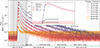 |
Fig. 1. Illustration of the method with which we determined the onset and peak times of an SEP event observed by SOHO/ERNE on May 28, 2021. The main panel shows time-intensity profiles across eight energy ranges (13−100 MeV), where the raw data are plotted as solid lines and the smoothed data are shown as dash-dotted lines. The gray shaded region denotes the search window for the peak identification. Identified peaks are marked by red circles. The inset zooms into the dashed region, displaying the onset determination for the 25−32 MeV range using the linear fitting method. The raw data points are shown as pink circles, and the blue circles represent the data points used for the linear fit. The solid black line shows the fit result. The horizontal red lines indicate the background level (solid line for the mean and dashed line for 3σ). The intersection of the black fitted line with the red background line defines the onset time. |
The most straightforward method for determining the peak time is to select the time corresponding to the maximum flux within a chosen interval. However, for high-resolution data, random fluctuations due to small statistics can introduce significant uncertainty. Therefore, we adopted an optimized algorithm for the peak identification: First, we applied a sliding median filter to the original flux time series to remove outlier data points, and we then smoothed the data using a Savitzky-Golay filter, which reduces high-frequency noise while preserving the waveform characteristics (Savitzky & Golay 1964; Schafer 2011). Within a defined search window for the peak, we set a prominence threshold equal to 0.3 times the variance of the smoothed data within that window, which helped us to distinguish the true main peak from minor fluctuations. Finally, we only accepted a candidate peak when the time interval to any adjacent peak was at least 5 minutes and its full width at half maximum exceeded 3 minutes. This ensured the identification of a physically reliable peak time. Despite the previous smoothing procedure used to identify the peak, the final peak time was identified from the 1-minute resolution data to capture the exact maximum.
3.3. Statistical analysis of the SEP rise time
Applying the method described above, we systematically extracted the rise time (Δt) for each energy channel and for each SEP event. Figures 2 and 3 present the statistical distribution histograms of the rise times in different energy channels as observed by Tianwen-1/MEPA and SOHO/ERNE, respectively, with the mean and standard deviation (SD) calculated for each energy channel. Figs. 2b–f shows that the distribution sharply increases at low rise-time values, followed by a decline toward higher rise-time values. This feature is not visible in other panels (at higher energies) because all histograms plotted here share the same bin width of 250 min to maintain consistency in the following analysis. The feature becomes visible when the bin width is smaller (not shown here) in the other panels of Figs. 2 and 3, however. To quantitatively describe the right-skewed shape of these distributions, a log-normal distribution was fitted to each histogram. The probability density function is given by
 (2)
(2)
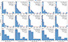 |
Fig. 2. Histograms of the rise times of SEP events observed by the Tianwen-1/MEPA instrument at the orbit of Mars in different energy channels. Panels (a)–(o) correspond to 15 energy intervals spanning 2−100 MeV. In each panel, the blue histogram (bin width fixed at 250 minutes) represents the rise time distributions, while the red curve shows the log-normal fitting of the distribution. The legend in each panel lists the number of events we analyzed, the mean and SD of the observed rise times, and the fitted log-normal parameters with the median and shape parameter defined in Eq. (2). |
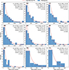 |
Fig. 3. Histograms of the rise times of SEPs observed by SOHO/ERNE in different energy channels. Panels (a)–(i) correspond to nine energy intervals spanning 13−100 MeV with a bin width of 200 minutes. The parameters shown in the legends are the same as in Fig. 2. |
where σ controls the dispersion, and eμ corresponds to the geometric mean, which equals the median in a log-normal distribution. In the legends of Figs. 2 and 3, parameter eμ is denoted as the median in the legends. The arithmetic mean and median values were then used for the power-law fits presented in Fig. 4.
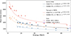 |
Fig. 4. Relation between the rise time Δt (y-axis) and particle energy E (x-axis) based on statistical observations from Earth and Mars. The diamonds and inverted-triangles represent the statistical mean and geometric mean from log-normal distribution fits, respectively. Red and yellow denote MEPA data, and dark green and light blue denote ERNE data. The purple and dark blue arrows indicate the mean and median rise time derived from TGO dose-rate measurements. |
The statistical results reveal the following facts: (1) The correlation between the rise time and the particle energy is strongly negative, that is, higher energies correspond to shorter rise times. For example, the average rise time of SEPs at Mars decreases from 882.53 minutes at the lowest energy (2 MeV) to 318.65 minutes at the highest energy (100 MeV). A similar trend is observed near Earth, with the rise time decreasing from 393.56 minutes at 13 MeV to 207.73 minutes at 100 MeV. (2) When we compare approximately the same energy intervals, the rise times near Mars are generally longer than those near Earth. This increase is consistent not only with the longer transport path at greater heliocentric distances, but also with the radial evolution of scattering conditions inferred from our analysis. These observational trends and their inferred dependences indicate underlying physical processes that we examine in Sect. 4.
4. Theoretical model based on observational results
4.1. SEP rise time derived from the pure diffusion model
A relatively complete description of the transport and modulation of SEPs in the expanding solar wind is described by the Fokker-Planck equation (Parker 1965),
![Mathematical equation: $$ \begin{aligned} \frac{\partial f}{\partial t} = -\frac{V_{\rm sw}}{r^2} \frac{\partial }{\partial r}(r^2 f) + \frac{2V_{\rm sw}}{3r} \frac{\partial }{\partial E}[f E n(E)] + \frac{1}{r^2} \frac{\partial }{\partial r}\left(\kappa r^2 \frac{\partial f}{\partial r}\right), \end{aligned} $$](/articles/aa/full_html/2026/06/aa60162-26/aa60162-26-eq3.gif) (3)
(3)
where f(r, E, t) represents the distribution of the particles in space, energy, and time; Vsw is the solar wind speed; κ is the diffusion coefficient; m0 is the rest mass of the particle; and n(E) represents the normalization conversion factor between particle momentum and kinetic energy, defined as n(E) = p dE/(E dp). For relativistic particles, n(E)≈1; and for nonrelativistic particles, n(E)≈2. The three terms on the right-hand side represent the key physical processes that govern SEP transport: convection, adiabatic cooling, and diffusion. Each of these transport mechanisms can modify the original acceleration characteristics of energetic particles.
Wang et al. (2022) simplified this equation under the assumptions of instantaneous impulsive injection and pure radial diffusion. Assuming that the radial diffusion coefficient follows a power-law form κ = κ0(r/r0)β with 0 ≤ β < 2, they obtained the solution
 (4)
(4)
where the parameter b and the dimensionless parameter c are given by
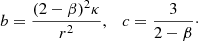 (5)
(5)
The rise time from onset to peak was then derived as
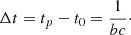 (6)
(6)
Further analysis by Wang et al. (2022) revealed an empirical power-law relation between the parameters b and c from observational fits c ∝ b−γ, with an observed value of γ ≈ 0.4 and a theoretical expectation of γ = 0.5. Based on their framework, we combined Eq. (6) with the relation c ∝ b−γ to derive the dependence of the rise time on the diffusion coefficient,
 (7)
(7)
This equation establishes the inverse power-law relation between the rise time and the diffusion coefficient, which we combine with the energy dependence of κ to derive the Δt − E scaling in the following subsection.
4.2. The relation between rise time and particle energy
According to quasi-linear theory (QLT) developed by Jokipii (1966), the perpendicular diffusion coefficient κ⊥ is usually much smaller than the parallel one κ∥ (Giacalone & Jokipii 1999). Numerical simulations further quantify this disparity, showing that the ratio κ⊥/κ∥ ranges from 10−1 to as low as 10−4 depending on the turbulence properties of the interplanetary medium (Conlon 1978; Dröge et al. 2010; Qin & Shalchi 2012). A comprehensive review of the analytical theories for perpendicular transport, including quasi-linear theory, nonlinear guiding center theory, and unified nonlinear transport theory, has been provided by Shalchi (2020). Furthermore, as discussed by Van den Berg et al. (2021), the drift and perpendicular diffusion mechanisms governing perpendicular transport of SEPs are two primary processes that operate in addition to parallel transport, and drift effects become apparent only > 2 hours after the event onset. Therefore, during the rise phase, radial diffusion is dominated by parallel diffusion along the magnetic field. Following Jokipii (1971), the radial diffusion coefficient can be expressed as
 (8)
(8)
where ψ is the angle between the radius vector from the Sun and the outward direction along the magnetic field, given by ψ = tan−1(rΩs/Vsw) (with Ωs = 2.9 × 10⁻⁶ sec−1 the rotation frequency of the Sun, and Vsw is the solar wind speed). Given that κ⊥ ≪ κ∥, we approximated κr ≈ κ∥cos2(ψ). Since the cos2(ψ) factor is purely geometric and does not introduce an additional energy dependence, we also absorbed this geometric factor into the proportionality constant and use κ ≈ κ∥ in the following derivation of the energy dependence.
In particle transport theory, the parallel diffusion coefficient can be expressed as (Jokipii 1971; Dröge et al. 2010)
 (9)
(9)
where v is the particle speed, and λ∥ is the parallel mean free path.
To establish the relation between Δt and Energy E, we examined the energy dependence of v and λ∥. The rest energy of a proton is E0 = 938 MeV and its kinetic energy is E. The total energy therefore is Etot = E + E0. When we define a dimensionless quantity x = E/E0, its speed in the relativistic regime is
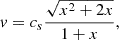 (10)
(10)
where cs denotes the speed of light.
Bieber et al. (1994) noted that the mean free path follows a power-law dependence on particle rigidity R,
 (11)
(11)
where the index α is linked to the background magnetic turbulence spectrum. Theoretically, the turbulence spectrum follows P(k)∝k−q and α = 2 − q. Classical Kolmogorov turbulence (q = 5/3) corresponds to α = 1/3, while the Iroshnikov-Kraichnan spectrum (q = 3/2) for magnetohydrodynamic turbulence gives α = 1/2 (Jokipii 1971; Qin et al. 2006; Wang & Qin 2015). Two extreme cases are the Bohm diffusion limit (maximum scattering, α = 1; see Hussein & Shalchi 2014 for a numerical investigation of strong turbulence) and rigidity-independence scattering (α ≈ 0) (Bieber et al. 1994; Palmer 1982; Chen et al. 2024). Based on ion observational data, Dröge (2000) reported a typical α ≈ 0.3 in the rigidity range of about 30 − 300 MV (corresponding to proton kinetic energies of approximately 0.5 − 47 MeV). Therefore, α typically ranges between 0 and 1, depending on the state of heliospheric turbulence.
When the proton rigidity is  , Eq. (11) becomes
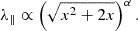 (12)
(12)
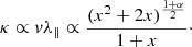
Combination of the expressions for speed and mean free path gives
 (13)
(13)
For protons, E0 = 938 MeV, so for normal SEPs with energies below about 100 MeV, we can assume that E ≪ E0 or x ≪ 1, which leads to  and 1 + x ≈ 1. The above equation becomes
 (14)
(14)
Substitution of this into Eq. (7) (the empirical correlation between Δt and κ) yields the final theoretical expression linking the rise time Δt to the particle energy and the turbulence parameter α,
 (15)
(15)
We further defined the power-law exponent η as Δt ∝ Eη, with η = −(1 − γ)(1 + α)/2. This formulation makes it evident that for typical values of γ and α, the rise time decreases with increasing particle energy. An empirical estimate of η derived from observational data is presented below.
4.3. Comparative analysis of the SEP rise time at Earth and Mars
Figure 4 shows the rise time as a function of proton energy based on multi-spacecraft observations. The SOHO/ERNE (dark blue lines) and Tianwen-1/MEPA (red and yellow lines) data points represent measurements of different energy, while the TGO dose-rate measurements (arrows) provide independent constraints on SEP rise time at higher energies. The TGO results are consistent with those from the Tianwen-1 MEPA data at high energies. This clearly confirms the reliability of our rise time analysis. However, since the dose rate records particles of all energies reaching the detector and does not have a clearly defined effective energy range, we did not include the TGO results in the power-law fit that is plotted as lines in the figure.
The power-law fit follows the form Δt ∝ Eη, which is consistent with the analytical solution of Eq. (15). We fitted η = −0.368 ± 0.058 near Earth and η = −0.302 ± 0.031 near Mars based on the mean rise time, where the uncertainties represent the 1σ statistical errors derived from the fitting procedure. Based on the median rise time, we have η = −0.325 ± 0.051 near Earth and η = −0.270 ± 0.029 near Mars. However, we note that due to the different energy limits of the different instruments, the fitted energy ranges differ between Earth (13−100 MeV) and Mars (2−100 MeV). The associated uncertainty in η could be better quantified if the energy coverage were harmonized and cross-instrument differences were accounted for in future work. Despite the uncertainties, the power-law exponent η is steeper at Earth than at Mars based on the mean and median results, indicating a stronger energy dependence of the rise time at 1 AU.
Based on the power-law relations between rise time and energy obtained from the fits in Fig. 4, we computed the difference in the rise times in the 5−100 MeV range at 1 MeV intervals between Mars and Earth. The rise time at Mars is approximately 137.13 minutes longer on average than that at Earth. Furthermore, the data and fitted functions reveal that the rate at which the rise time decreases with increasing energy gradually flattens at higher energies. This behavior can be understood in terms of energy losses during radial propagation. As a direct manifestation of particle transport, the rise time is sensitive to the particle speed and its evolution with distance. Cao et al. (2025) demonstrated that the particle flux decreases with distance as f(R)∝R−ϕ(E), where the decay index ϕ(E) declines with increasing energy. Consequently, lower-energy particles lose more energy during transport through processes such as diffusion and adiabatic cooling, resulting in a greater reduction in speed and thus a prolonged rise time, while higher-energy particles lose less energy and exhibit shorter rise times. At sufficiently high energies, the energy losses become negligible compared to the total energy of particles, and the rise time is primarily governed by the velocity, exhibiting only a weak dependence on energy.
While energy-loss considerations offer a qualitative understanding of the observed relation between rise time and energy, we provide a quantitative interpretation within the framework of a parallel diffusion model. Adopting the theoretical relation η = −(1 − γ)(1 + α)/2 derived in Eq. (15) and assuming γ = 0.5 as theoretically expected considering primarily the diffusion process (Wang et al. 2022), we inverted the observed power-law exponents to obtain the turbulence parameter α. The uncertainty in α can be propagated from the fitting error of η via
 (16)
(16)
Using the statistical uncertainty of η from the mean-value fits, we obtain α = 0.472 ± 0.232 at Earth and α = 0.208 ± 0.124 at Mars. The geometric-mean fits yield very similar results: α = 0.3 ± 0.204 at Earth and α = 0.08 ± 0.116 at Mars. The difference between α derived from observations at Earth and Mars indicates a considerable weakening of the rigidity dependence on the parallel mean free path with increasing radial distance. The lower α value at Mars suggests that turbulence in this region is more similar to a rigidity-independent scattering regime than that near Earth.
This radial evolution of α reflects fundamental changes in the properties of the solar wind turbulence. As the distance increases, the break frequency separating the inertial range from the dissipation range shifts toward lower frequencies in the fast and slow solar wind (Bruno & Trenchi 2014; Duan et al. 2018, 2020; Lotz et al. 2023). Consequently, at a fixed particle gyro-frequency, the sampled turbulence spectral index q becomes larger, leading to a reduction in α via α = 2 − q.
This radial evolution can be assessed by comparing the turbulence spectra observed during the SEP event on March 28, 2025. In this event, Earth and Mars were nearly aligned along the same magnetic field line, providing a unique opportunity to isolate the radial evolution of turbulence. Figure 5 presents the PSD of magnetic field fluctuations at Earth (Wind-MFI) and Mars (Tianwen1-MOMAG). For statistical reliability, we analyzed 4-hour intervals of magnetic field data that encompass the onset time of the SEP event at both locations. As shown in panel c, the spectral indices at Earth are −1.13 in the lower-frequency range (likely corresponding to the inertial range) and −2.24 in the higher-frequency range (approaching the dissipation range). At Mars, the spectrum is systematically steeper, with indices of −1.57 and −2.76 in the lower- and higher-frequency ranges, respectively. This feature is consistent with the lower α value derived from the rise time obtained for Mars in Sect. 4.3. However, the break frequency at Mars is higher than that at Earth during this event, which differs from the aforementioned radial evolution trend based on solar wind observations. This discrepancy can be explained by energy injection in the Martian upstream solar wind. As noted by Marino & Sorriso-Valvo (2023), such an injection (possibly driven by pickup ions or foreshock waves) can induce inverse cascades, which enhance dissipation at smaller scales (higher frequencies) and thus shift the break frequency toward higher values.
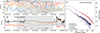 |
Fig. 5. Comparison of the PSD of the magnetic field at Earth and Mars during the SEP event on March 28, 2025. Panels (a) and (b) show the three components of the magnetic field and the total field magnitude observed by Wind (near Earth) and Tianwen-1 (near Mars), respectively. The gray area marks the 4-hour interval (which encompasses the onset time of the SEP event) of the magnetic field data used for the PSD analysis shown in panel (c), where the blue and red lines represent the PSD of magnetic field fluctuations at Earth and Mars, respectively. The orange lines indicate the fitted slopes in the inertial and dissipation ranges, with the corresponding spectral indices labeled nearby. |
Beyond this single event, the diversity of turbulence spectra observed near Mars provides a broader statistical context for the radial trend inferred from our SEP analysis of the rise time. Zou et al. (2025) classified the magnetic PSD upstream of Mars into three types (types A, B, and C) based on spectral morphology. Type A spectra exhibit a well-developed inertial range followed by a dissipation range, resembling those commonly observed near Earth. Energy cascades through the inertial range and dissipates via ion-scale mechanisms, such as cyclotron damping (Chen et al. 2014). Type B spectra show evidence of energy injection at some scales, resulting in a steeper dissipation range. Type C spectra lack a distinct dissipation range, suggesting that dissipation might occur at frequencies beyond the observational window. Notably, only about one-quarter of the events at Mars display type A spectra similar to those near Earth, while over one-third fall into type B and another third into type C (Zou et al. 2025). The radial shift of the dissipation range was further supported by Cheng & Wang (2022), who found that the Taylor scale, which marks the transition from the inertial range to the dissipation range, is smaller by approximately one order of magnitude in the upstream solar wind of Mars than at Earth. These studies suggested that a substantial fraction of the solar wind magnetic field exhibits intrinsically steeper spectra at Mars due to break frequency shift and/or different turbulence regimes (energy injection or absence of a dissipation range). Therefore, the lower α we derive at Mars is consistent with a steeper effective turbulence spectrum, regardless of whether it is caused by a transition into the dissipation range or by fundamentally different spectral morphologies.
Several additional factors might further contribute to the observed radial trend. The weakening of the interplanetary magnetic field with distance, together with possible changes in its anisotropic structure, alters the resonance-matching conditions between waves and particles, and it thereby weakens the rigidity dependence of the scattering efficiency. These processes jointly lead to a particle transport behavior that approaches a rigidity-independent regime.
In addition to the power-law analysis presented above, the rise time data from TGO and MEPA shown in Fig. 4 can be used to examine the characteristic energy at which the radiation dose and particle flux are correlated strongest in the Mars orbit. The TGO AB dose measurements yield a mean rise time of 294.5 min and a median of 223.0 min, as shown in the figure. A comparison of these values with the power-law curves obtained from fitting the MEPA data (the mean fit y = 1337.81E−0.302 ± 0.031 and the geometric mean fit y = 786.11E−0.270 ± 0.029) gives intersection energies of 150.15 MeV and 106.31 MeV, respectively. Propagating the uncertainty in the power-law exponent η yields energy ranges of [94.1, 266.3] MeV for the mean and [67.6, 186.2] MeV for the median. These ranges can be considered as the main SEP proton energy range contributing to the radiation dose measured by TGO orbiting Mars. On the other hand, the TGO data provide an important high-energy constraint of the relation between rise time and energy.
5. Discussion and conclusion
We examined a series of SEP events observed by the SOHO/ERNE (near Earth) and Tianwen-1/MEPA (near Mars) instruments between November 2020 and March 2025. We selected 75 events in Earth orbit and 58 events in Mars orbit that satisfied our identification criteria. For each event, we used the linear fitting method to determine the onset time and an optimized peak-finding algorithm to extract the peak time. We provided statistical estimates of the relation between the rise time and particle energy.
Under the assumptions of instantaneous injection of source particles and pure radial diffusion, where parallel diffusion dominates during the rise phase, we derived the theoretical relation Δt ∝ E−(1 − γ)(1 + α)/2 from the diffusion model. On the other hand, observations show that the rise time follows a distinct power-law dependence on energy: we derived Δt ∝ E−0.368 ± 0.058 near Earth and Δt ∝ E−0.302 ± 0.031 near Mars. Inverting the turbulence parameter α through η = −(1 − γ)(1 + α)/2, we inferred α = 0.472 ± 0.232 at Earth and α = 0.208 ± 0.124 at Mars. The lower α value at Mars indicates that the mean free path is less dependent on rigidity with increasing distance. This trend agrees with the turbulence evolution: while turbulence near Earth is predominantly in the inertial range, it shifts toward a regime that is dominated by the dissipation range and is more independent of the rigidity scattering at larger distances (about 1.5 AU).
Our model relies on several simplifying assumptions that might introduce uncertainties into the inverted parameters. A key assumption is the instantaneous particle injection, which does not capture the complexity of acceleration at coronal mass ejection (CME)-driven shocks. In diffusive shock acceleration, particles gradually gain energy through repeated interactions with the shock front, with higher-energy particles requiring longer acceleration times (Drury 1983; Blandford & Eichler 1987). This energy-dependent acceleration time naturally leads to a scenario in which higher-energy particles are released later than lower-energy ones, which might cause the recent observations of inverse-velocity arrival detected by the Parker Solar Probe and Solar Orbiter (e.g., Li et al. 2025; Chen et al. 2025). On the other hand, CME-driven shocks can extend particle acceleration over prolonged periods, leading to a continuous injection of SEPs (e.g., Reames 1999; Desai & Giacalone 2016). As the shock propagates outward into the interplanetary space, its strength gradually decreases. This reduces the maximum energy attainable by accelerated particles while continuously accelerating particles to lower energies. Together, these effects tend to prolong the observed rise times, more likely at lower energies, leading to a steeper inferred energy dependence (η in Δt ∝ Eη) and a potential overestimation of the turbulence parameter α compared to the instantaneous-injection scenario.
Second, the diffusion model we employed mainly considers parallel diffusion along the mean magnetic field. However, parallel and perpendicular diffusion both operate during SEP transport in reality, and the degree of magnetic connectivity varies from one event to the next. When the spacecraft is poorly connected to the acceleration point, perpendicular diffusion across field lines can become an essential transport process. Neglecting this mechanism might bias the inferred transport parameters, particularly for poorly connected events. Furthermore, the apparent rise time reflects not only local scattering conditions, but more importantly, the time required for particles to propagate across field lines, in particular, during poorly connected events. This adds further complexity to its interpretation.
Third, the pure diffusion model we employed does not explicitly include adiabatic cooling. While adiabatic cooling does not directly affect the rise time itself, it might play a crucial role in shaping the particle energy spectrum during propagation (Wang & Guo 2024). As demonstrated by Cao et al. (2025), adiabatic cooling modulates the rate at which the particle flux decreases with distance, leading to a radial dependence on spectral hardening that varies with the source spectrum. This energy-dependent modulation might alter the relative arrival times of particles at different energies, thereby affecting the power-law exponent η, and consequently, the inferred turbulence parameter α. In Sect. 4.3, we invoked this effect to qualitatively account for the observed reduction in η. However, a more complete assessment would require a transport model that simultaneously accounts for diffusion, adiabatic cooling, and their interplay.
Last but not least, the selection of events and the peak-detection algorithm, though objective in procedure, retain some subjectivity in parameter choices, which might bias the rise-time statistics in some way. Nevertheless, the use of the rise time instead of the absolute flux reduces the effect of cross-calibration uncertainties and provides a new perspective for our understanding of the transport features of SEPs at different heliospheric distances.
Despite these uncertainties associated with the model assumptions, the observed power-law relations between the rise time and energy at Earth and Mars are statistically significant and represent a reliable observation result. The clear radial evolution of the power-law exponent η and the derived turbulence parameter α suggests that the underlying physical trend, namely the weakening of the rigidity dependence with radial distance, is unlikely to be an artifact of the model simplifications. Nevertheless, as the interpretation is based on a diffusion model that neglects certain key physical processes, it is subject to quantitative uncertainties. More refined models incorporating finite injection of the particle source, perpendicular diffusion, and adiabatic cooling are essential for separating the contributions of the source and transport processes.
Future studies might focus on detailed case-by-case analyses of well-connected SEP events to examine the variation in the rise time profiles with energy and magnetic connection geometry, thereby providing specific constraints on local turbulence parameters. Moreover, combining multi-satellite observations (e.g., Parker Solar Probe, Solar Orbiter, BepiColombo, and outer-heliosphere missions) would enable us to construct a radius-dependent profile of the turbulence parameter α. Such a multi-point approach would help us to separate the radial evolution of turbulence from event-to-event variations and to verify turbulent transport models of SEPs in the heliosphere. These might serve as important tools for predicting space weather.
Acknowledgments
The authors acknowledge the support by the National Natural Science Foundation of China (Grant Nos. 42130204, 42188101, 42521007, 42474221) and the National Key R&R Program of China (2025YFF0510900) The Level-2 archived data from both the MEPA and MOMAG instruments onboard Tianwen-1 are publicly available through the Planetary Exploration Project Science Data Release System at (https://moon.bao.ac.cn/). In addition, the MOMAG data are also accessible via the official website of MOMAG team at the University of Science and Technology of China (USTC, http://space.ustc.edu.cn/dreams/tw1_momag/).
References
- Bieber, J. W., Matthaeus, W. H., Smith, C. W., et al. 1994, ApJ, 420, 294 [Google Scholar]
- Blandford, R., & Eichler, D. 1987, Phys. Rep., 154, 1 [Google Scholar]
- Bruno, R., & Carbone, V. 2013, Liv. Rev. Sol. Phys., 10, 2 [Google Scholar]
- Bruno, R., & Trenchi, L. 2014, ApJ, 787, L24 [NASA ADS] [CrossRef] [Google Scholar]
- Cao, Y., Wang, Y., & Guo, J. 2025, A&A, 695, A25 [NASA ADS] [CrossRef] [EDP Sciences] [Google Scholar]
- Chen, C., Leung, L., Boldyrev, S., Maruca, B., & Bale, S. 2014, Geophys. Res. Lett., 41, 8081 [NASA ADS] [CrossRef] [Google Scholar]
- Chen, X., Giacalone, J., Guo, F., & Klein, K. G. 2024, ApJ, 965, 61 [NASA ADS] [CrossRef] [Google Scholar]
- Chen, X., Zhao, L., Giacalone, J., et al. 2025, ApJ, 994, 242 [Google Scholar]
- Cheng, L., & Wang, Y. 2022, ApJ, 941, 37 [Google Scholar]
- Chiappetta, F., Laurenza, M., Lepreti, F., & Consolini, G. 2021, ApJ, 915, 8 [NASA ADS] [CrossRef] [Google Scholar]
- Conlon, T. F. 1978, J. Geophys. Res.: Space Phys., 83, 541 [Google Scholar]
- Desai, M., & Giacalone, J. 2016, Liv. Rev. Sol. Phys., 13, 3 [NASA ADS] [CrossRef] [Google Scholar]
- Domingo, V., Fleck, B., & Poland, A. I. 1995, Sol. Phys., 162, 1 [Google Scholar]
- Dröge, W. 1994, IAU Colloq. 142: Solar Cosmic Rays, 142, 567 [Google Scholar]
- Dröge, W. 2000, ApJ, 537, 1073 [CrossRef] [Google Scholar]
- Dröge, W., Kartavykh, Y., Klecker, B., & Kovaltsov, G. 2010, ApJ, 709, 912 [CrossRef] [Google Scholar]
- Drury, L. O. 1983, Rep. Prog. Phys., 46, 973 [Google Scholar]
- Duan, D., He, J., Pei, Z., et al. 2018, ApJ, 865, 89 [NASA ADS] [CrossRef] [Google Scholar]
- Duan, D., Bowen, T. A., Chen, C. H., et al. 2020, ApJS, 246, 55 [Google Scholar]
- Farwa, G., Dresing, N., Vuorinen, L., et al. 2025, Adv. Space Res., 77, 1304 [Google Scholar]
- Giacalone, J., & Jokipii, J. 1999, ApJ, 520, 204 [Google Scholar]
- Guo, J., Wang, B., Whitman, K., et al. 2024, Adv. Space Res., https://doi.org/10.1016/j.asr.2024.03.070 [Google Scholar]
- Heras, A., Sanahuja, B., Smith, Z., Detman, T., & Dryer, M. 1992, ApJ, 391, 359 [NASA ADS] [CrossRef] [Google Scholar]
- Heras, A. M., Sanahuja, B., Lario, D., et al. 1995, ApJ, 445, 497 [NASA ADS] [CrossRef] [Google Scholar]
- Horbury, T. S., Forman, M., & Oughton, S. 2008, Phys. Rev. Lett., 101, 175005 [Google Scholar]
- Hu, J., Li, G., Ao, X., Zank, G. P., & Verkhoglyadova, O. 2017, J. Geophys. Res.: Space Phys., 122, 10 [Google Scholar]
- Hussein, M., & Shalchi, A. 2014, ApJ, 785, 31 [Google Scholar]
- Huttunen-Heikinmaa, K., Valtonen, E., & Laitinen, T. 2005, A&A, 442, 673 [NASA ADS] [CrossRef] [EDP Sciences] [Google Scholar]
- Iroshnikov, P. 1964, Sov. Astron., 7, 566 [Google Scholar]
- Jokipii, J. R. 1966, ApJ, 146, 480 [Google Scholar]
- Jokipii, J. 1971, Rev. Geophys., 9, 27 [Google Scholar]
- Kahler, S. W., & Ling, A. G. 2017, Sol. Phys., 292, 59 [Google Scholar]
- Kolmogorov, A. N. 1941, Numbers. In Dokl. Akad. Nauk SSSR, 30, 301 [Google Scholar]
- Kolmogorov, A. N. 1991, Proc. R. Soc. London A, 434, 9 [Google Scholar]
- Kraichnan, R. H. 1965, Phys. Fluids, 8, 1385 [Google Scholar]
- Krimigis, S. M. 1965, J. Geophys. Res., 70, 2943 [Google Scholar]
- Krucker, S., & Lin, R. 2000, ApJ, 542, L61 [CrossRef] [Google Scholar]
- Lario, D., Aran, A., Gómez-Herrero, R., et al. 2013, ApJ, 767, 41 [CrossRef] [Google Scholar]
- Laurenza, M., Consolini, G., Storini, M., Pallocchia, G., & Damiani, A. 2016, J. Phys. Conf. Ser., 767, 012015 [Google Scholar]
- Lepping, R., Acũna, M., Burlaga, L., et al. 1995, Space Sci. Rev., 71, 207 [NASA ADS] [CrossRef] [Google Scholar]
- Li, G., Zhao, L., Wang, L., Liu, W., & Wu, X. 2020, ApJ, 900, L16 [NASA ADS] [CrossRef] [Google Scholar]
- Li, C., Tang, S., Hu, X., et al. 2021, Space Sci. Rev., 217, 26 [Google Scholar]
- Li, Y., Guo, J., Pacheco, D., et al. 2025, Natl. Sci. Rev., 12, nwaf348 [Google Scholar]
- Lotz, S., Nel, A., Wicks, R., et al. 2023, ApJ, 942, 93 [NASA ADS] [CrossRef] [Google Scholar]
- Marino, R., & Sorriso-Valvo, L. 2023, Phys. Rep., 1006, 1 [NASA ADS] [CrossRef] [Google Scholar]
- Meyer, P., Parker, E., & Simpson, J. 1956, Phys. Rev., 104, 768 [NASA ADS] [CrossRef] [Google Scholar]
- Pallocchia, G., Laurenza, M., & Consolini, G. 2017, ApJ, 837, 158 [Google Scholar]
- Palmer, I. 1982, Rev. Geophys., 20, 335 [NASA ADS] [CrossRef] [Google Scholar]
- Parker, E. N. 1965, Planet. Space Sci., 13, 9 [Google Scholar]
- Qin, G., & Shalchi, A. 2012, Adv. Space Res., 49, 1643 [NASA ADS] [CrossRef] [Google Scholar]
- Qin, G., Zhang, M., & Dwyer, J. 2006, J. Geophys. Res.: Space Phys., 111, A08101 [Google Scholar]
- Reames, D. V. 1999, Space Sci. Rev., 90, 413 [NASA ADS] [CrossRef] [Google Scholar]
- Savitzky, A., & Golay, M. 1964, J. Anal. Chem., 36, 1627 [Google Scholar]
- Schafer, R. W. 2011, IEEE Signal Process. Mag., 28, 111 [NASA ADS] [CrossRef] [Google Scholar]
- Semkova, J., Koleva, R., Benghin, V., et al. 2018, Icarus, 303, 53 [Google Scholar]
- Shalchi, A. 2020, Space Sci. Rev., 216, 23 [NASA ADS] [CrossRef] [Google Scholar]
- Tang, S., Wang, Y., Zhao, H., et al. 2020, Earth Planet. Phys., 4, 355 [Google Scholar]
- Torsti, J., Valtonen, E., Lumme, M., et al. 1995, Sol. Phys., 162, 505 [CrossRef] [Google Scholar]
- Van den Berg, J., Engelbrecht, N., Wijsen, N., & Strauss, R. 2021, ApJ, 922, 200 [NASA ADS] [CrossRef] [Google Scholar]
- Wang, Y., & Guo, J. 2024, A&A, 691, A54 [NASA ADS] [CrossRef] [EDP Sciences] [Google Scholar]
- Wang, Y., & Qin, G. 2015, ApJ, 806, 252 [NASA ADS] [CrossRef] [Google Scholar]
- Wang, Y., Lyu, D., Wu, X., & Qin, G. 2022, ApJ, 940, 67 [NASA ADS] [CrossRef] [Google Scholar]
- Wang, Y., Zhang, T., Wang, G., et al. 2023, Earth Planet. Phys., 7, 216 [Google Scholar]
- Whitman, K., Egeland, R., Richardson, I. G., et al. 2023, Adv. Space Res., 72, 5161 [NASA ADS] [CrossRef] [Google Scholar]
- Wilks, D. S. 2011, Stat. Meth. Atmos. Sci., 100, 2 [Google Scholar]
- Xie, H., Mäkelä, P., Gopalswamy, N., & St. Cyr, O. 2016, J. Geophys. Res.: Space Phys., 121, 6168 [NASA ADS] [CrossRef] [Google Scholar]
- Yu, B., Chi, Y., Owens, M., et al. 2023, ApJ, 953, 105 [NASA ADS] [Google Scholar]
- Zhang, M., Qin, G., & Rassoul, H. 2009, ApJ, 692, 109 [NASA ADS] [CrossRef] [Google Scholar]
- Zou, Z., Wang, Y., Zhang, T., et al. 2023, Sci. China Technol. Sci., 66, 2396 [Google Scholar]
- Zou, Z., Wang, Y., Su, Z., et al. 2025, ApJ, 988, 76 [Google Scholar]
All Figures
|
Fig. 1. Illustration of the method with which we determined the onset and peak times of an SEP event observed by SOHO/ERNE on May 28, 2021. The main panel shows time-intensity profiles across eight energy ranges (13−100 MeV), where the raw data are plotted as solid lines and the smoothed data are shown as dash-dotted lines. The gray shaded region denotes the search window for the peak identification. Identified peaks are marked by red circles. The inset zooms into the dashed region, displaying the onset determination for the 25−32 MeV range using the linear fitting method. The raw data points are shown as pink circles, and the blue circles represent the data points used for the linear fit. The solid black line shows the fit result. The horizontal red lines indicate the background level (solid line for the mean and dashed line for 3σ). The intersection of the black fitted line with the red background line defines the onset time. |
| In the text | |
|
Fig. 2. Histograms of the rise times of SEP events observed by the Tianwen-1/MEPA instrument at the orbit of Mars in different energy channels. Panels (a)–(o) correspond to 15 energy intervals spanning 2−100 MeV. In each panel, the blue histogram (bin width fixed at 250 minutes) represents the rise time distributions, while the red curve shows the log-normal fitting of the distribution. The legend in each panel lists the number of events we analyzed, the mean and SD of the observed rise times, and the fitted log-normal parameters with the median and shape parameter defined in Eq. (2). |
| In the text | |
|
Fig. 3. Histograms of the rise times of SEPs observed by SOHO/ERNE in different energy channels. Panels (a)–(i) correspond to nine energy intervals spanning 13−100 MeV with a bin width of 200 minutes. The parameters shown in the legends are the same as in Fig. 2. |
| In the text | |
|
Fig. 4. Relation between the rise time Δt (y-axis) and particle energy E (x-axis) based on statistical observations from Earth and Mars. The diamonds and inverted-triangles represent the statistical mean and geometric mean from log-normal distribution fits, respectively. Red and yellow denote MEPA data, and dark green and light blue denote ERNE data. The purple and dark blue arrows indicate the mean and median rise time derived from TGO dose-rate measurements. |
| In the text | |
|
Fig. 5. Comparison of the PSD of the magnetic field at Earth and Mars during the SEP event on March 28, 2025. Panels (a) and (b) show the three components of the magnetic field and the total field magnitude observed by Wind (near Earth) and Tianwen-1 (near Mars), respectively. The gray area marks the 4-hour interval (which encompasses the onset time of the SEP event) of the magnetic field data used for the PSD analysis shown in panel (c), where the blue and red lines represent the PSD of magnetic field fluctuations at Earth and Mars, respectively. The orange lines indicate the fitted slopes in the inertial and dissipation ranges, with the corresponding spectral indices labeled nearby. |
| In the text | |
Current usage metrics show cumulative count of Article Views (full-text article views including HTML views, PDF and ePub downloads, according to the available data) and Abstracts Views on Vision4Press platform.
Data correspond to usage on the plateform after 2015. The current usage metrics is available 48-96 hours after online publication and is updated daily on week days.
Initial download of the metrics may take a while.