


| Issue |
A&A
Volume 710, June 2026
|
|
|---|---|---|
| Article Number | A268 | |
| Number of page(s) | 12 | |
| Section | Extragalactic astronomy | |
| DOI | https://doi.org/10.1051/0004-6361/202659801 | |
| Published online | 19 June 2026 | |
Testing X-ray periodicity and the long-term trend in PG 1553+113 via targeted Swift-XRT monitoring
1
Department of Physics and Astronomy, Clemson University, Kinard Lab of Physics, Clemson, SC 29634-0978, USA
2
Department of Astronomy, University of Virginia, P.O. Box 400325 Charlottesville, VA 22904, USA
3
Deutsches Elektronen-Synchrotron DESY, Platanenallee 6, 15738 Zeuthen, Germany
4
IPARCOS and Department of EMFTEL, Universidad Complutense de Madrid, E-28040, Madrid, Spain
5
Julius-Maximilians-Universität Würzburg, Fakultät für Physik und Astronomie, Emil-Fischer-Str. 31, D-97074 Würzburg, Germany
★ Corresponding authors: This email address is being protected from spambots. You need JavaScript enabled to view it.
; This email address is being protected from spambots. You need JavaScript enabled to view it.
; This email address is being protected from spambots. You need JavaScript enabled to view it.
Received:
11
March
2026
Accepted:
7
April
2026
Abstract
Context. PG 1553+113 is a blazar with the most significantly detected periodic pattern in its multiwavelength (MWL) emission, making it one of the most promising candidates for hosting a supermassive black hole binary.
Aims. The presence of this periodic behavior in the X-ray band remains under debate, largely due to the lack of continuous monitoring. This has led to differing conclusions across previous studies. We examined whether the recently identified linear long-term trends in the γ-ray and optical bands also exist in the X-ray regime.
Methods. We evaluated the ∼2.1-year period in the X-ray light curve of PG 1553+113 using two dedicated monitoring campaigns with Swift-XRT and UVOT, guided by predictions of future oscillation phases. We also examined whether the long-term trend is present in X-rays, the potential periodic behavior of the X-ray power-law photon index, and its potential correlation with the X-ray flux.
Results. We find tentative evidence for a correlation between the predicted high-emission states in the γ-ray band and those observed in the X-ray and UV bands. However, we do not find strong evidence of the same periodic pattern in the X-ray band. In addition, we find that the X-ray light curve is consistent with the presence of a long-term linear trend, in agreement with those previously reported in the γ-ray, optical, and radio bands.
Conclusions. Overall, these results indicate that the X-ray emission likely shares the same long-term behavior observed in the γ-ray and optical bands. Nevertheless, the pronounced stochastic variability that characterizes the X-ray light curve limits our ability to draw firm conclusions regarding the presence of this periodic behavior.
Key words: methods: data analysis / galaxies: active / BL Lacertae objects: individual: PG 1553+113
GECO Fellow.
© The Authors 2026
 Open Access article, published by EDP Sciences, under the terms of the Creative Commons Attribution License (https://creativecommons.org/licenses/by/4.0), which permits unrestricted use, distribution, and reproduction in any medium, provided the original work is properly cited.
This article is published in open access under the Subscribe to Open model. This email address is being protected from spambots. You need JavaScript enabled to view it. to support open access publication.
1. Introduction
PG 1553+113 is a BL Lacertae (hereafter BL Lac) object and one of the most extensively studied blazars due to its distinctive long-term variability across multiple wavelengths (Albert et al. 2007). It is located at a redshift of z≈0.433 (Johnson et al. 2019; Dorigo Jones et al. 2022), and its emission spans the entire electromagnetic spectrum, from radio to very high-energy γ rays (e.g., Ackermann et al. 2015; Peñil et al. 2024b; MAGIC Collaboration 2024). It is classified as a high-frequency–peaked BL Lac object (HBL), because the peak of its synchrotron spectral energy distribution lies in the UV–X-ray band (e.g., Padovani & Giommi 1995; Abdo et al. 2010a). As a consequence, the X-ray emission of PG 1553+113 is dominated by synchrotron radiation from the highest-energy electrons in the jet.
A particularly notable feature of PG 1553+113 is the periodic behavior observed in its γ-ray emission. Early analyses of Fermi-LAT (Fermi Large Area Telescope) data reported a significant periodicity of approximately 2.1 years, with the number of identified cycles ranging from approximately four to seven, depending on the time span of the analyzed light curve (e.g., Ackermann et al. 2015; Peñil et al. 2020; Rico et al. 2025). Interestingly, this periodic signature is not limited to the γ-ray band; similar periodicities have also been detected in the optical, UV, and radio bands, with approximately four (radio) to eight (optical) cycles identified depending on the data available for each energy band (e.g., Ackermann et al. 2015; Peñil et al. 2024b; MAGIC Collaboration 2024), pointing to a common physical mechanism modulating the emission across these wavelengths.
In addition to this periodicity, a new long-term trend has recently been identified. Multiwavelength (MWL) observations reveal a gradual, approximately linear increase in flux over time in the γ-ray, UV, optical, and radio bands (Peñil et al. 2024b). The slope of this increasing trend appears to be consistent across all these energy bands, suggesting a coherent long-term process influencing the entire spectral energy distribution. Gao et al. (2023) propose that it is part of another periodic oscillation with a period of 42 years. To explore the potential origin of this trend, Adhikari et al. (2024) analyzed more than a century of historical optical data, uncovering a possible secondary periodicity of ∼22 years. This finding implies that the variability of PG 1553+113 may be governed by more than one characteristic timescale.
While the ∼2.1-year periodicity is well established in the γ-ray, UV, and optical bands, the behavior in the X-ray regime remains more ambiguous. Several studies propose different periodicities in the Swift-XRT (X-Ray Telescope) light curve of PG 1553+113. For instance, Huang et al. (2021) report a 2.1-year period, consistent with that observed in the higher and lower energy bands. In contrast, Peñil et al. (2024b) find evidence for a shorter 1.5-year period with a significance of approximately 2.8σ1, as well as a secondary period of 2.3 years, also at 2.8σ1 significance. Aniello et al. (2024) observe a period of 1.4 years. These discrepancies suggest that the Swift-XRT X-ray emission is likely governed by additional or distinct variability mechanisms compared to other wavebands. In particular, the X-ray light curve may be dominated by strong stochastic variability, which can either obscure an underlying periodic pattern or render the emission effectively consistent with red-noise-dominated behavior, thereby reducing the detectability of a coherent periodic signal (e.g., Vaughan 2005; Marscher 2014; Zhang et al. 2015; Petropoulou et al. 2018).
Understanding these differences is essential to advance our knowledge of the variability patterns of PG 1553+113. In particular, unraveling the connection between the X-ray and γ-ray variability is key to constraining models of emission processes, jet structure, and central engine dynamics (e.g., Zhang & Böttcher 2013; Osorio-Archila et al. 2025).
This paper presents a comprehensive analysis of the long-term X-ray variability of PG 1553+113 and explores its correlation with the observed γ-ray and UV activity. Our goal was to provide new insights into the temporal properties of this blazar, contributing to a better understanding of its broadband variability.
To achieve this, we conducted a targeted observational campaign using Swift-XRT and UVOT (Ultraviolet/Optical Telescope). Specifically, we designed two monitoring programs that aimed to capture the X-ray behavior during the expected high-emission phases, as predicted by extrapolating the period of ∼2.1-year modulation previously observed in MWL data. We strategically scheduled these observations to coincide with predicted maxima in the γ-ray light curve, which allowed us to investigate whether a similar periodic pattern is present in the X-ray band and to assess the degree of cross-band coherence. Additionally, these observations provide an opportunity to better characterize any long-term trends in the X-ray emission, analogous to those reported in the MWL variability.
This paper is organized as follows. In Section 2, we introduce the different theoretical models proposed to explain the periodic emission of PG 1553+113. Section 3 presents the Swift observational campaigns aimed at evaluating the presence of the 2.1-year modulation in the X-ray band. In Section 4, we describe the data reduction and analysis procedures used to construct the MWL light curves. Section 5 outlines the different techniques and methods employed to investigate the long-term variability of the light curves. We present the results obtained from the application of these methodologies in Section 6. Section 7 provides a discussion of these results. We summarize the main conclusions of this work in Section 8.
2. Theoretical models
Several models have been proposed to explain the MWL periodic variability of PG 1553+113. Most of these models are based on a supermassive black hole binary (SMBHB) scenario. A common interpretation for the observed ∼2.1-yr period is a SMBHB at sub-parsec separations, whose orbital dynamics modulate the emission through accretion-flow perturbations or geometric changes in the jet orientation (e.g., Ackermann et al. 2015; Caproni et al. 2017; Sobacchi et al. 2017; Tavani et al. 2018; Abdollahi et al. 2024). Among these possibilities, jet precession is one of the most discussed mechanisms (Camenzind & Krockenberger 1992). In this model, the secondary black hole exerts a torque on the accretion disk, inducing the disk precession and the relativistic jet. The resulting periodic changes in the viewing angle can then produce strong flux variations through Doppler boosting (Villata & Raiteri 1999).
In the context of PG 1553+113, Gao et al. (2023) propose a model based on jet precession (without specifying its cause), where the jet rotates with constant angular velocity around an axis. This causes the Doppler factor of the jet to vary over time, leading to periodic changes in flux. This scenario reproduces both the observed periodicity and the rising trend observed in the γ-ray light curves. Caproni et al. (2017) propose two different models. The first model assumes a single jet launched by the primary black hole, with its precession driven by the gravitational influence of the secondary black hole. In the alternative model, both black holes launch their own jets, and the observed variability results from the interaction and combined emission of these precessing jets. Similarly, Sobacchi et al. (2017) also use the periodicity produced by jet precession due to the orbital motion of the jet-emitting SMBH around its companion.
Tavani et al. (2018) explain the periodic oscillation in terms of an orbiting binary system. In addition to the main peaks of the periodic oscillations, the study identifies secondary peaks, named “twin peaks”, which occur symmetrically around the main peaks. The authors propose two scenarios to interpret these observations. In the first, we observe the jet of the primary SMBH, and the secondary black hole induces additional instabilities in the primary jet during its orbital motion, leading to the observed twin peaks. In the second model, the secondary black hole launches its own precessing jet, contributing to the twin peaks observed in the emission profile.
Precession can also arise from other mechanisms. For instance, in single SMBH systems, Lense-Thirring precession induced by misalignment between the black hole spin axis and the disk angular momentum vector can lead to periodic modulation of the jet orientation (Franchini et al. 2016; Zanazzi & Lai 2019).
In binary systems, tidal forces from the secondary black hole can further enhance accretion rate oscillations by periodically disturbing the outer disk. These modulations may imprint themselves on the jet emission (Gracia et al. 2003). In this context, Abdollahi et al. (2024) suggest that the companion object triggers a Keplerian orbital modulation in the accretion rate onto the primary SMBH. This interaction leads to periodic hydrodynamic variability, characterized by repeated enhancements in the primary’s accretion disk activity and the corresponding emission from its relativistic jet.
Adhikari et al. (2024) explain the observed long-term trend and the secondary period of ∼22 years. They interpret the dual periodicities reported for PG 1553+113 within a binary SMBH framework: they attribute the shorter ∼2.1-year period to the orbital motion of the SMBH pair, while they associate the longer ∼22-year modulation with the dynamics of an over-dense structure (termed a “lump”) in the circumbinary accretion disk (D’Orazio et al. 2015). Hydrodynamic simulations of circumbinary disks (Westernacher-Schneider et al. 2022) predict these lumps and show that tidal interactions with the binary can drive the formation of nonaxisymmetric density enhancements. Additional studies, such as Farris et al. (2014), showed that such disks can develop long-lived, rotating overdensities that exert variable torques on the binary system and modulate the inflow of matter through the disk cavity. The interaction between the binary and the lump can result in periodic enhancements in accretion rate onto the binary system, which in turn can produce large-scale modulations in the emitted flux.
These previous scenarios imply different expectations for the MWL variability. In geometric models, such as jet precession, the modulation is primarily produced by periodic changes in the viewing angle and therefore in the Doppler boosting factor (Camenzind & Krockenberger 1992; Villata & Raiteri 1999; Rieger 2004). In this case, bands produced in closely related jet regions are expected to show coherent long-term variability with small lags, although the modulation amplitude may remain energy dependent (Villata & Raiteri 1999; Rieger 2004). Within this framework, the optical and UV emission as well as the γ-ray emission may display similar recurrence patterns (MAGIC Collaboration 2024; Peñil et al. 2024b), whereas the radio emission can respond later because it is often produced further downstream in a more extended and partially self-absorbed region of the flow (Max-Moerbeck et al. 2014).
By contrast, in accretion-driven binary scenarios, the orbital motion modulates the mass supply and thus the power injected into the jet through periodic perturbations of the accretion flow (Lai & Muñoz 2023; Abdollahi et al. 2024). In such models, the resulting MWL signal may show broader flares, band-dependent amplitudes, and possible delays associated with the propagation of disturbances from the disk to the jet-emitting regions (Lai & Muñoz 2023). In addition, circumbinary-disk models based on the lumps can results in lags between the different bands (Farris et al. 2014; Lai & Muñoz 2023). For PG 1553+113, these expectations are especially relevant because the available MWL data indicate that the optical variability strongly correlates with the γ-ray modulation (e.g., Ackermann et al. 2015; Peñil et al. 2024b), and is consistent with no lag, whereas the radio emission appears correlated but delayed, and the X-ray behavior is less clearly correlated with the long-term γ-ray oscillation (Ackermann et al. 2015; Peñil et al. 2024b). Overall, this phenomenology is broadly consistent with a scenario in which at least part of the modulation is geometric and jet-related (Madero & Domínguez 2026), while additional accretion-driven effects may also contribute to shaping the long-term variability (Farris et al. 2014; Adhikari et al. 2024).
3. Swift observations
Several independent studies have confirmed the robust period nature of the MWL emission (Ackermann et al. 2015; MAGIC Collaboration 2024; Peñil et al. 2024b; Abdollahi et al. 2024). However, as noted previously, the periodicity in the X-ray band remains a subject of debate due to the conflicting results reported across different analyses (Huang et al. 2021; Peñil et al. 2024b; Aniello et al. 2024).
3.1. Periodicity in the literature
Periodic behavior in blazar emissions is typically classified into two categories: quasiperiodic oscillations (QPOs) and strict periodicity. These classifications are not only observationally motivated but also mathematically distinct. Quasiperiodic oscillations (QPOs) refer to variability patterns that show a preferred timescale of oscillation but with a significant stochastic (unpredictable) element. As a result, while a characteristic timescale may be identified, precise prediction of future oscillations is inherently uncertain. By contrast, strict periodicity implies a deterministic pattern, allowing for the reliable prediction of future behavior. Given the inconsistency among the X-ray studies, the variability observed in this band for PG 1553+113 is more appropriately characterized as a QPO rather than a strictly periodic signal, whereas strict periodicity has been confirmed in all other wavebands (Ackermann et al. 2015; Peñil et al. 2024b).
To address this ambiguity and test whether the X-ray emission follows a genuinely periodic pattern, we developed two dedicated observing campaigns with the Swift-XRT instrument. We designed these campaigns to specifically target epochs when a high X-ray flux would be expected if the emission followed the same periodicity observed in the γ-ray band (with a period of ∼2.1 years). By focusing on predicted high states based on this periodic model, our approach allows for a direct test of phase coherence and recurrence in the X-ray regime. Successful detection of X-ray peaks aligned with the predicted epochs would strengthen the case for a common physical origin driving the periodicity across energy bands, while deviations would support the interpretation of the X-ray variability as stochastic or independently modulated.
3.2. Observational campaigns and archival data
The first observational campaign (Program ID: 1821168, PI: Peñil, 12 observations) took place during cycle 18 of Swift, coincident with the expected peak of emission in March 2023 (±1 month, based on our analysis of the Fermi data Rico et al. 2025). We monitored PG 1553+113 for a total of four months around its predicted high state. We monitored the source bi-weekly for one month, then weekly for two months (i.e., one month on each side of the expected peak position), and then returned to bi-weekly monitoring for another month. This resulted in a total of 12 observations, each with a duration of 1 ks.
The second campaign (Program ID: 2124062, PI: Peñil, 24 observations) took place during Swift cycle 21, coincident with an expected peak of emission in May 2025 (±1 month, based on our analysis of the Fermi data Rico et al. 2025). In this case, we monitored PG 1553+113 weekly for three months (April, May, and June), totaling 12 observations that align with the emission peak and its uncertainty. During other observable months (July-September 2025; January 2025–February 2026), Swift monitored the source bi-weekly.
In addition to our observational campaigns, Swift observed PG 1553+113 on 5552 occasions, between October 18, 2014 and September 25, 2025. The majority of these observations contain event files for both photon counting (PC) and window-timing (WT) modes, with a total of 404 and 420 event files, respectively. We included all available observations in our initial analysis.
4. Data analysis
We analyzed the Swift-XRT and Swift-UVOT data using the Swift Analysis Pipeline for Light curve Extraction (SAPLE)3. We retrieved Fermi-LAT γ-ray data from the public-light curve repository (Abdollahi et al. 2023)4. We describe the detailed analysis procedures for each instrument in the following subsections.
4.1. XRT data analysis
We used Swift-XRT data (Burrows et al. 2005) and extracted spectra in the 0.3−10 keV band, as is the default in SAPLE. The core of the pipeline consists of four codes, which we ran as described in the documentation.
The first code, xrtpipeline_run.py, runs the official HEASoft5 command xrtpipeline on all observations, including the photon-counting (PC) and the windowed-time (WT) observations. As a second step, we opened one of the XRT images of the target and selected default circular source and background regions of 50” and 90”, respectively, for PC events and 50” and 50” for WT events. We centered the source region on the target location, whereas we chose the background region in a source-free region close to the target.
The second code, xrt_make_image.py, produces images of all observations, together with the corresponding source and background regions used for spectral extraction. To ensure that the source is always at the center of the source circle, the code automatically centroids the circle and saves a new source region for each observation. We then visually inspected these images for evident issues in each observation (e.g., the source region missing the source, the background region containing contaminant sources, or empty event files). We discarded a total of three observations at this point due to the presence of artifacts (see Appendix C for details and examples).
After removing problematic observations, we ran the third code, xselect_run.py. This code creates spectra for both the source and background regions selected. Finally, the fourth code, xspec_pl_fit.py, performs the following steps for each observation. In the first step, it uses the xrtmkarf task to produce an ancillary response file, and it then uses grppha to assign the corresponding background, ancillary response file (ARF) and response matrix file (RMF6) to the source spectra. Next, it rebins the spectra using the optimal binning scheme provided by ftgrouppha. Finally, it fits a redshifted power-law model corrected for Galactic absorption (tbabs*zpowerlaw in XSPEC, using the wilm abundances, Wilms et al. 2000) to the obtained spectrum using Cash statistics (C-stat) and extracts the following information: count-rate, observed and intrinsic flux (corrected for galactic absorption, taken to be 3.61 × 1020 cm−2, HI4PI Collaboration 2016) and associated uncertainties, photon index and associated uncertainties, and a goodness of fit estimator (i.e., C-stat over degrees of freedom).
Of the 817 analyzed archival XRT observations, 34 have non-positive counts, 154 do not have convergent fits, and 41 have non-convergent error estimations. All of these issues trace back to a lack of signal-to-noise ratio7 in the WT observations. We obtain a total of 585 usable data points after the analysis. We present the XRT light curve in the second panel of Fig. 1, highlighting the two predicted emission peaks targeted by the monitoring campaigns. We used the photon index data in Sect. 6.
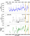 |
Fig. 1. Multiwavelength light curves of PG 1553+113 used in this study. The vertical orange bands mark the approximate locations of the Swift monitoring campaigns that targeted the predicted high-emission states. Top: Fermi-LAT light curve (30-day binning). Center: Swift-XRT light curve, including both PC and WT observations. Bottom: UVOT UV band light curve (uvv filter). The analysis uses data from MJD ∼55 000 onward to avoid potential inconsistencies associated with the large data gap prior to that date (Peñil et al. 2025e). |
4.2. UVOT data analysis
We used data from Swift-UVOT 8, considering all available filters9 for each observation. We used the SAPLE codes dedicated to UVOT analysis as follows. To begin, we ran uvot_src_bkg_regions.py to create source and background regions (5” and 30” circles, respectively) for all observations, as well as create images of the FOV. Similar to the XRT pipeline, we visually inspected all images to remove problematic observations. Specifically, UVOT images can be affected by imperfect tracking, causing streaks in the images or event files, and resulting in incorrect photometry. We removed a total of 28 observations from the analysis (see Appendix C for details and examples).
After this, we ran uvotsource_run.py, which executes the standard uvotsource task to extract the source and background magnitude for each observation in all available filters. Finally, we ran uvotsource_extract_flux.py, which performs the following tasks. First, it corrects the AB magnitudes for Galactic extinction following the prescription in Roming et al. (2009). We took the extinction values (E(B–V)) for the source from Willingale et al. (2013)10. The code then transforms the corrected magnitudes and corresponding uncertainties into flux values. We chose to perform the analysis in magnitudes.
We started from 3052 photometric data points (considering all filters available per observation). Removing 28 observations resulted in the loss of 152 photometric points, leaving a total of 2900. As an example, we show the data for the UV band (from the “uvv” filter) in the bottom panel of Fig. 1.
4.3. Fermi-LAT data
We used the γ-ray data from the open-access Fermi-LAT light curve repository, which provides comprehensive data covering approximately 18 years of Fermi-LAT observations. For this study, we selected the 30-day binned light curves, using a fixed photon index. We chose this binning interval to facilitate the search for a period of ≈2.1 years and the long-term trend. Figure 1 (top) presents the Fermi-LAT light curve used in this study.
5. Methodology
We performed three types of variability analyses: periodicity searches, cross-correlation studies, and trend characterization. We describe the specific methodologies applied to each case in detail in the following.
5.1. Periodicity search
To carry out the periodicity search, we selected methods that are well suited to the specific challenges of the X-ray light curve. In particular, the X-ray light curve is characterized by irregular sampling, data gaps, and strong flaring activity, all of which can significantly affect periodicity searches. Peñil et al. (2025d,e) provide a systematic study of these effects and quantify the impact of flares and gaps on the detection and significance of periodic oscillations. We therefore restricted our analysis to methods whose statistical performance was directly characterized under these observational conditions. Consequently, we did not include other techniques, such as the weighted wavelet Z-transform (WWZ, Foster 1996), as this was not calibrated in these previous studies.
For these reasons, we used the generalized Lomb–Scargle periodogram (GLSP; Zechmeister & Kürster 2009), the singular spectrum analysis (SSA; Greco et al. 2016; Nina Golyandina 2020), and the phase dispersion minimization (PDM; Stellingwerf 1978). The GLSP extends the traditional Lomb–Scargle Periodogram (Lomb 1976; Scargle 1982) by explicitly incorporating measurement uncertainties into the power calculation. By considering these uncertainties, the GLSP accounts for data errors in periodic signals, thereby enhancing the reliability of the period estimates.
The SSA method is designed to decompose a time series into its fundamental components, allowing the distinction between structured signals and noise. In practice, the method first embeds the light curve into a trajectory matrix constructed from lagged copies of the original series, where the embedding dimension is set by the window length. This matrix is then decomposed through singular value decomposition into a set of components, each representing a different mode of variability. Periodic or quasiperiodic signals are typically associated with a component that shows the oscillatory structure of the light curve, whereas stochastic fluctuations are usually captured by other components. By reconstructing the deterministic component associated with the candidate oscillation, SSA reduces the influence of noise and transient features such as flares, making periodic patterns easier to identify in the original light curve. After isolating the oscillatory component from the stochastic ones, we applied the LSP to the reconstructed signal. This two-step approach improves the robustness of the period search and helps quantify the associated uncertainties (Rico et al. 2025).
Finally, PDM offers a complementary approach: it tests trial periods by minimizing the scatter (dispersion) of phase-folded data, making it well-suited for detecting non-sinusoidal periodicities that may be missed by Fourier-based techniques, such as LSP.
The significance of the potential period reported by these methods is assessed by generating 100 000 artificial light curves that replicate the characteristics of the original light curve, including its sampling pattern, power spectral density (PSD), and the probability distribution function of the original data. To this end, we applied the method of Emmanoulopoulos et al. (2013). We modeled the PSD of each light curve segment using a power-law function of the form A * f−β+C, where A is the normalization factor, β is the spectral index, f denotes frequency, and C represents the Poisson noise level. We estimated the model parameters are estimated via maximum likelihood estimation, supported by a Markov chain Monte Carlo (MCMC) analysis11.
5.2. Correlation
To analyze correlations in unevenly sampled data, we applied the z-transformed discrete correlation function (z-DCF; Alexander 2013), a method specifically developed to handle irregular time sampling. Unlike the standard discrete correlation function, the z-DCF reduces the bias associated with uneven observational cadences. This approach allowed us to estimate time lags between the γ-ray emission and the X-ray and UV bands. We estimated the significance of the correlations using the same approach as in the periodicity study.
5.3. Trend characterization
To characterize the trend, we used the methodology presented in Peñil et al. (2025c)12. As estimated in Peñil et al. (2024b), the trend associated with the emission of PG 1553+113 is linear. Consequently, we employed a linear regression13, to characterize the parameters of the linear trend.
We also used the R-squared (R2) criterion to evaluate how well the trend fits the data. This metric quantifies the proportion of the variance in the dependent variable that can be explained by the independent variable(s) in a regression model. The R2 values range from 0 to 1, with higher values indicating that the model accounts for a greater portion of the observed data variability. However, what constitutes a good R2 depends on the context and specific objectives of the analysis. There is no absolute cutoff, as acceptable levels may vary across fields. According to Hair et al. (2011), R2 values of 0.25, 0.50, and 0.75 are typically indicate weak, moderate, and substantia fits, respectively.
6. Results
As an initial step, we assessed the accuracy of our predictions for the high-emission states of PG 1553+113. Fig. 1 shows that the results are mostly consistent with expectations. During Swift cycle 18, the γ-ray flux reached its maximum between February and May 2023, coinciding with an X-ray peak observed between April and May 2023. The UVOT data also exhibits a flux maximum during the same period, around April 2023. For Swift cycle 21, the γ-ray shows irregular oscillations with maximum emission between December 2024 and September 2025. The expected X-ray maximum is less clearly defined than in the previous oscillation, likely as a consequence of the intrinsically irregular flux variability in the X-ray band. In contrast, the UV emission exhibits a more coherent behavior, with a peak at comparable epochs. Taken together, these monitoring campaigns provide tentative confirmation of the predictions for the γ-ray behavior based on its ∼2.1-year periodicity, with consistent behavior observed in the UV band at comparable epochs, but no clear corresponding pattern in the X-rays for the second predicted peak.
6.1. Periodicity
Table A.1 lists the results of the periodicity analysis. In the γ-ray band, we recover the significant (> 3σ) well-established ∼2.1-year period, consistent with previous detections in the literature (e.g., Ackermann et al. 2015; Peñil et al. 2024b, 2025a).
In the UV band (uvv filter), we performed two complementary analyses: one using a 30-day binned light curve, matched to the γ-ray binning to facilitate a direct interband comparison and another using the unbinned data to preserve the original temporal sampling and evaluate the effect of short-timescale variability. The use of a binned light curve provides advantages for periodicity studies, since binning suppresses part of the short-timescale stochastic variability, reduces the impact of isolated fluctuations and observational scatter, and enhances the visibility of long-term coherent modulations. We used a binning method based on the median value within each bin, which previous studies have shown to be effective (e.g., Rani et al. 2013; Peñil et al. 2024a). In both cases, we recover the same characteristic period (∼2.1 yr), although with markedly different significance: > 3σ for the binned light curve, but only ∼1σ for the unbinned data. This difference highlights the strong impact of short-lived variability on the significance estimate, despite the stability of the recovered period. These results are consistent with previous studies (Peñil et al. 2024b; MAGIC Collaboration 2024).
For the X-ray band, we performed two independent analyses using both the unbinned and the 30-day binned light curves. The unbinned data reveal a nonsignificant period of ∼1.5 years, consistent with the findings of Peñil et al. (2024b) and Aniello et al. (2024). However, as discussed in Sect. 5, these results may be significantly affected by the intrinsic properties of the X-ray light curve, particularly the presence of gaps and strong flaring states.
For gaps, ∼90% of the X-ray light curve date are missing when compared with an ideal, evenly daily sampled series in which every time bin contains a measurement. Such a large fraction of missing data severely reduces the ability of all methods to detect genuine periodicity, often leading to suppressed signals or spurious detections (Adhikari et al. 2025; Peñil et al. 2025e). As a result, the apparent period could simply be an artifact of the gap distribution in the light curve. To evaluate this hypothesis, we used the test from Adhikari et al. (2024, 2025), Peñil et al. (2025e). This approach involves simulating 100,000 synthetic light curves using the method described in Emmanoulopoulos et al. (2013), maintaining the same PSD, PDF, and gap structure (percentage and temporal structure) as the original light curve. The resulting distribution of recovered periods and significances provides a benchmark to identify potential biases toward certain timescales that might align with the detected signal. In addition, we quantified how often the simulations reproduce the same period–significance combination observed in the real light curve. We define an occurrence as one in which the recovered period falls within the uncertainty range of the real-data result and its significance exceeds that measured in the observed light curve. As Fig. B.1 shows, the GLSP test indicates that the detected period is most likely driven by the gap structure, with a coincidence rateof ∼10% in the simulations.
In contrast, analysis of the binned X-ray light curve yields different results, with a nonsignificant hint (< 2σ) of a ∼2.5-year period. Several factors could explain the absence of a statistically significant ∼2.1-year signal in this case. Here, compared with an ideal evenly sampled series, the fraction of gaps decreases to ∼30%, which lies below the commonly adopted 50% threshold above which gaps strongly bias periodicity searches (Peñil et al. 2025e). To further assess the role of gaps, we applied the same test that was used for the unbinned light curve. The results, shown in Fig. B.1, indicate that while the gap distribution could in principle contribute to the appearance of the ∼2.5-year feature, this explanation is unlikely: the coincidence rate between the observed result and the simulations is 0.5%.
Therefore, the dominant factor likely affecting the inference of a ∼2.1-year period could be the intrinsic variability of the X-ray emission itself, particularly the impact of high-flux states and strong flaring activity. During these episodes, irregular flux variations can mask or distort the underlying periodic signals, leading to a substantial reduction in the apparent significance of long-term oscillations. In extreme cases, both the inferred period and its significance can be affected by uncertainties exceeding 100% (Peñil et al. 2025d).
Overall, the combined influence of gaps and flaring states likely explains the weaker and less consistent detection of long-term periodicity in the X-ray band. Despite the tentative indications of a ∼2.1-year modulation in the X-ray band, we cannot infer that the X-ray emission of PG 1553+113 follows the same periodic pattern observed at other wavelengths. Extending this effort over longer timescales will allow us to observe additional candidate peaks, providing the statistical leverage needed to clarify the nature of the X-ray variability and resolve the remaining uncertainties.
6.2. Correlation
Analysis of the γ-ray and X-ray emissions reveals a correlation between the two bands. In particular, we measure a time lag of −12 ± 21 days (consistent with zero lag) with a significance of 2.8σ. Given the 30-day binning adopted for the Fermi-LAT light curve, time lags within ±30 days remain compatible with a zero-delay scenario. This result is consistent with previous analyses, which report a near-zero lag at comparable significance levels (∼3.0σ; Peñil et al. 2024b) and with the findings of Dhiman et al. (2021).
In addition, we restricted the analysis to the X-ray observations obtained during the specific observational windows defined by our Swift proposals. Under these conditions, the resulting cross-correlation is again consistent with a zero time lag, with a significance of 2.4σ, further supporting a contemporaneous variability between the X-ray and γ-ray emissions during these intervals.
For the cross-correlation between the UV and γ-ray bands, we obtain results consistent with a zero time lag, with a measured delay of −11 ± 21 days with a significance of 3.0σ, consistent with Peñil et al. (2024b). When we restrict the analysis to the peak intervals covered by our observations, the cross-correlation remains consistent with zero lag but with a reduced significance of 1.7σ. This decrease in significance is likely related to the most recent γ-ray oscillation, which exhibits a complex double-peaked structure. When combined with the temporal gaps in the UV coverage, this complexity can dilute the correlation signal and limit the statistical significance of the result.
We used the Bayesian blocks shown in Fig. 2 to highlight the high-emission states of both the γ-ray and X-ray light curves. In the X-ray panel, most high-emission states appear incomplete, except for the interval coincident with our first observational campaign (cycle 18; Sect. 3.2). Despite these gaps, most γ-ray high-emission states have an X-ray counterpart, with two apparent exceptions: the peak around MJD ∼58 000 and the high-emission state predicted for cycle 21 (§3.2). In the UV band, Fig. B.2 shows the corresponding counterparts to the γ-ray high-emission states.
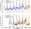 |
Fig. 2. Bayesian blocks of Fermi-LAT and Swift-XRT light curves. The vertical gray lines approximately mark the high-emission states corresponding to the inferred period of ≈2.1 years, while the vertical orange lines approximately indicate the Swift monitoring campaign designed t to track the predicted high states. |
6.3. Trend characterization
Fig. 3 shows the estimation of the long-term trends in the X-ray band. The best-fit slope is 35 ± 8 × 10⁻⁵ with R2 = 77.1%, consistent with the value of ∼20 × 10−5 reported by Peñil et al. (2024b). The inclusion of the new X-ray observations confirms the presence of a persistent upward trend in the X-ray emission of PG 1553+113.
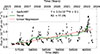 |
Fig. 3. Trend decomposition of the X-ray data. The green line shows the underlying trend extracted using seasonal_decompose. The trend covers a shorter time span than the full light curve duration because of decomposition method. The red line shows the fit to this trend; the dashed red line extends the fit line across the full light curve. The R2 value is 77.2%, indicating a good fit. |
In the γ-ray band, we obtain a slope of 70 ± 7 × 10⁻⁵, with R2 = 81.3% (Fig. B.3), consistent with Peñil et al. (2025c). For the UV data, the slope is 20 ± 1 × 10⁻⁵, with R2 = 76.8% (Fig. B.3), which is also compatible with previous results (Peñil et al. 2024b).
These results demonstrate that the X-ray, γ ray, and UV bands all exhibit linear long-term trends with different slopes. This multiband agreement strengthens the case for a common underlying physical mechanism driving the gradual brightening of PG 1553+113, as proposed by Adhikari et al. (2024).
6.4. Relation between photon index and flux
We also performed a study of the X-ray flux and the photon index (see Sect. 4.1). Fig. B.4 shows the evolution of these quantities. To investigate possible relationships between these quantities, we applied a Bayesian blocks analysis to both the X-ray flux and the associated photon index. Figure 4 shows an apparent anticorrelation between the X-ray flux and the photon index. This behavior becomes more evident when considering the two monitoring cycles separately: during the high-emission flare of cycle 18, the PL index exhibits a clear depression (e.g., harder photon index for brighter flux state), whereas in cycle 21 the X-ray flux displays relatively lower emission, while the PL index reaches high (softer) values.
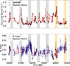 |
Fig. 4. Bayesian blocks of the X-ray flux and the power-law index from the fitting model. An apparent anti-correlation is visible between the flux and the associated PL index. The vertical gray lines mark the high-emission states corresponding to the inferred period of ≈2.1 years, while the vertical orange lines indicate the Swift monitoring campaign designed to track the predicted high states. |
To further quantify this, we performed a z-DCF correlation analysis between the two datasets, finding an anti-correlation consistent with a near-zero time lag (–7 ± 12 days), with a significance of 2.2σ.
To complement the z-DCF analysis, we examined the relationship between the X-ray flux and the photon index using Spearman’s rank correlation coefficient (Spearman 2010), ρS. Spearman’s ρS can be applied to irregularly sampled time series, provided the two observables are evaluated as one-to-one paired measurements at common epochs. For the X-ray flux and photon-index light curves we obtain ρS = –0.6209. We assessed the significance with Monte Carlo simulations by constructing the null distribution of ρS from M = 105 pairs of surrogate light curves that reproduce the sampling pattern and variability properties of the data. The surrogate distribution is centered near zero, with median  and a central 68% interval of [ − 0.0668, 0.0663]. This implies that chance correlations under the adopted null model typically satisfy |ρS|≲0.07. The observed anticorrelation exceeds all surrogate realizations, yielding a two-sided surrogate-based p-value of psurr = 10−5 and demonstrating that the flux–index anticorrelation is highly significant relative to the red-noise hypothesis.
7. Discussion
One of our main results is the confirmation of our predictions for the next high-emission states of PG 1553+113 in the γ ray band. We forecast two γ-ray maxima, in March 2023 (cycle 18) and May 2025 (cycle 21), with an uncertainty of one month. Fig. 1 shows that the γ-ray light curve displays peaks near May 2023 and June 2025, in agreement with these forecasts. The UV emission also shows consistent behavior. This outcome highlights the value of using forward predictions as an independent test of candidate periodic patterns. The rationale behind this approach is straightforward: a stochastic process, by definition, cannot be reliably predicted beyond its statistical properties, whereas a genuine periodic signal should allow for reproducible forecasts of future variability. If the predicted maxima or minima of the emission are confirmed by subsequent observations, this provides strong evidence that the variability is not simply the product of noise or chance fluctuations. In particular, it motivates the design of targeted observational campaigns aimed at monitoring epochs when the periodic model forecasts significant changes in emission.
In the X-ray band, some peaks appear to coincide with the γ-ray and UV activity, while for others the correspondence is uncertain, particularly for the high-emission state targeted in the cycle 21 proposal. As a result, establishing the same periodic behavior in X-rays remains challenging. However, we confirm the presence of the long-term trend in X-ray emission. The detection of consistent behavior across multiple wavelengths suggests a common origin for the MWL emission, and thus a common physical mechanism driving the variability. The trend itself lends additional support to the so-called lump scenario proposed for PG 1553+113. Nevertheless, further investigation is needed to fully assess the presence of the putative 22-year modulation.
The observed anticorrelation between the X-ray flux and the photon index in PG 1553+113 is consistent with the well-known harder-when-brighter behavior commonly observed in HBL BL Lac objects (e.g., Wang et al. 2018). Since the X-ray emission in this source is dominated by synchrotron radiation from the highest-energy electrons in the jet, an increase in flux accompanied by a hardening of the photon index can be interpreted as enhanced particle acceleration or fresh injection of high-energy electrons, which temporarily hardens the electron energy distribution and shifts the synchrotron peak to higher energies (Zhang et al. 2015). This behavior was previously reported for PG 1553+113 in MWL campaigns (MAGIC Collaboration 2024). The near-zero time lag between the flux and spectral variations further supports a scenario in which both quantities are driven by closely coupled acceleration and cooling processes within the same emitting region (Zhang et al. 2015). In addition, the highest-energy electrons in the jet have short radiative cooling and acceleration timescales and are therefore highly sensitive to localized and transient dissipation processes, such as magnetic reconnection or turbulent acceleration Petropoulou et al. (2018), Christie et al. (2019). As a result, the X-ray light curve is often dominated by rapid, large-amplitude fluctuations that introduce strong red-noise variability (Vaughan 2005). This enhanced stochastic component can substantially reduce the coherence and statistical significance of any underlying multi-year modulation in the X-ray band. In contrast, the γ-ray emission may arise from a more spatially extended or temporally averaged particle population within the jet, or from emission zones less affected by rapid cooling (Ghisellini et al. 2005; Marscher 2014), allowing dynamical modulations to remain detectable. Under these conditions, correlated high-emission states can coexist with a γ-ray periodicity and an apparently nonperiodic X-ray behavior, either because the periodic component is subdominant in X-rays or because the X-ray emission originates from a more intermittent, multi-zone substructure than the γ-ray emission.
Consequently, coordinated observational campaigns guided by predictions of future high-emission states are crucial, given the strong stochastic variability that characterizes the X-ray band. They provide a more effective strategy for testing whether the periodic behavior observed in the γ-ray and UV bands is also present in X-rays. Confirmation of such a connection with more evidence would strongly support the presence of a common physical mechanism driving variability across all these bands. Specifically, coupling between the γ-ray and X-ray bands would point to a scenario in which both components arise from the same leptonic population of relativistic electrons. In this framework, the X-ray emission is produced via synchrotron radiation, while the γ-ray photons originate from the upscattering of these synchrotron seed photons through the synchrotron self-Compton (SSC) mechanism (e.g., Abdo et al. 2010b). The correlated behavior between γ rays and the UV bands further supports this picture, as the UVOT flux traces the high-energy end of the synchrotron component that seeds the SSC process. Therefore, simultaneous or near-simultaneous variability in the UV, X-ray, and γ-ray domains naturally emerges from the dynamical evolution of a single electron population within a common emitting zone.
8. Summary
We investigated the X-ray emission of PG 1553+113, a well-studied blazar and a leading candidate for hosting a supermassive black hole binary. We aimed to assess whether the X-ray band reproduces the variability patterns, periodic modulation, and long-term trend previously reported at other wavelengths. To this end, we conducted two dedicated monitoring campaigns targeting predicted high-emission epochs using Swift-XRT. We did not find significant evidence for the ∼2.1-year period in X-rays. However, targeted observational campaigns during predicted high-emission states (based on the γ-ray periodicity) reveal hints of ∼0-lag correlation associated with X-ray flaring episodes. In addition, we confirm the presence of a long-term trend in the X-ray band, consistent with results from other energy ranges. Regarding the UV band, we find significant evidence of the ∼2.1-year (∼3.0σ) oscillations and ∼0-lag cross-correlation with the γ-ray band (∼3.0σ). These findings strengthen the hypothesis of a common physical origin for the MWL emission of PG 1553+113. Nevertheless, confirming the ∼2.1-year periodicity in X-rays will require continued monitoring guided by predictions of future oscillations, since such confirmation of a periodic pattern by applying natural periodicity-search strategies is not robust due to the intrinsically highly variable and irregularly distributed X-ray emission.
Acknowledgments
P.P. and M.A. acknowledge funding under NASA contract 80NSSC20K1562. L.M. acknowledges that this work was supported by the the Initiative and Networking Fund of the Helmholtz Association under the Helmholtz Investigator Groups Programme, call 2025 (VH-NG-21-01). LM acknowledges support from DESY (Zeuthen, Germany), a member of the Helmholtz Association HGF. This work was supported by the European Research Council, ERC Starting grant MessMapp, S.B. Principal Investigator, under contract no. 949555, and by the German Science Foundation DFG, research grant “Relativistic Jets in Active Galaxies” (FOR 5195, grant No. 443220636).
References
- Abdo, A. A., Ackermann, M., Agudo, I., et al. 2010a, ApJ, 716, 30 [NASA ADS] [CrossRef] [Google Scholar]
- Abdo, A. A., Ackermann, M., Ajello, M., et al. 2010b, ApJ, 708, 1310 [Google Scholar]
- Abdollahi, S., Ajello, M., Baldini, L., et al. 2023, ApJS, 265, 31 [NASA ADS] [CrossRef] [Google Scholar]
- Abdollahi, S., Baldini, L., Barbiellini, G., et al. 2024, ApJ, 976, 203 [Google Scholar]
- Ackermann, M., Ajello, M., Albert, A., et al. 2015, ApJ, 813, L41 [NASA ADS] [CrossRef] [Google Scholar]
- Adhikari, S., Peñil, P., Westernacher-Schneider, J. R., et al. 2024, ApJ, 965, 124 [CrossRef] [Google Scholar]
- Adhikari, S., Peñil, P., Domínguez, A., et al. 2025, MNRAS, 540, 1449 [Google Scholar]
- Albert, J., Aliu, E., Anderhub, H., et al. 2007, ApJ, 654, L119 [NASA ADS] [CrossRef] [Google Scholar]
- Alexander, T. 2013, ArXiv e-prints [arXiv:1302.1508] [Google Scholar]
- Aniello, T., Antonelli, L. A., Tombesi, F., et al. 2024, A&A, 686, A300 [NASA ADS] [CrossRef] [EDP Sciences] [Google Scholar]
- Burrows, D. N., Hill, J. E., Nousek, J. A., et al. 2005, Space Sci. Rev., 120, 165 [Google Scholar]
- Camenzind, M., & Krockenberger, M. 1992, A&A, 255, 59 [NASA ADS] [Google Scholar]
- Caproni, A., Abraham, Z., Motter, J. C., & Monteiro, H. 2017, ApJ, 851, L39 [NASA ADS] [CrossRef] [Google Scholar]
- Christie, I. M., Petropoulou, M., Sironi, L., & Giannios, D. 2019, MNRAS, 482, 65 [Google Scholar]
- Dhiman, V., Gupta, A. C., Gaur, H., & Wiita, P. J. 2021, MNRAS, 506, 1198 [NASA ADS] [CrossRef] [Google Scholar]
- D’Orazio, D. J., Haiman, Z., Duffell, P., Farris, B. D., & MacFadyen, A. I. 2015, MNRAS, 452, 2540 [CrossRef] [Google Scholar]
- Dorigo Jones, J., Johnson, S. D., Muzahid, S., et al. 2022, MNRAS, 509, 4330 [NASA ADS] [Google Scholar]
- Emmanoulopoulos, D., McHardy, I. M., & Papadakis, I. E. 2013, MNRAS, 433, 907 [NASA ADS] [CrossRef] [Google Scholar]
- Farris, B. D., Duffell, P., MacFadyen, A. I., & Haiman, Z. 2014, ApJ, 783, 134 [NASA ADS] [CrossRef] [Google Scholar]
- Foster, G. 1996, AJ, 112, 1709 [NASA ADS] [CrossRef] [Google Scholar]
- Franchini, A., Lodato, G., & Facchini, S. 2016, MNRAS, 455, 1946 [NASA ADS] [CrossRef] [Google Scholar]
- Gao, Q.-G., Lu, F.-W., Qin, L.-H., et al. 2023, ApJ, 945, 146 [Google Scholar]
- Ghisellini, G., Tavecchio, F., & Chiaberge, M. 2005, A&A, 432, 401 [CrossRef] [EDP Sciences] [Google Scholar]
- Gracia, J., Peitz, J., Keller, C., & Camenzind, M. 2003, MNRAS, 344, 468 [Google Scholar]
- Greco, G., Kondrashov, D., Kobayashi, S., et al. 2016, in Astrophys. Space Sci. Proc., 42, 105 [Google Scholar]
- Hair, J., Ringle, C., & Sarstedt, M. 2011, J. Market. Theory Practice, 19, 139 [Google Scholar]
- HI4PI Collaboration (Ben Bekhti, N., et al.) 2016, A&A, 594, A116 [NASA ADS] [CrossRef] [EDP Sciences] [Google Scholar]
- Huang, S., Yin, H., Hu, S., et al. 2021, ApJ, 922, 222 [NASA ADS] [CrossRef] [Google Scholar]
- Johnson, S. D., Mulchaey, J. S., Chen, H.-W., et al. 2019, ApJ, 884, L31 [NASA ADS] [CrossRef] [Google Scholar]
- Lai, D., & Muñoz, D. J. 2023, ARA&A, 61, 517 [NASA ADS] [CrossRef] [Google Scholar]
- Lomb, N. R. 1976, Ap&SS, 39, 447 [Google Scholar]
- Madero, E., & Domínguez, A. 2026, A&A, 707, L18 [NASA ADS] [CrossRef] [EDP Sciences] [Google Scholar]
- MAGIC Collaboration (Abe, H., et al.) 2024, MNRAS, 529, 3894 [Google Scholar]
- Marscher, A. P. 2014, ApJ, 780, 87 [Google Scholar]
- Max-Moerbeck, W., Hovatta, T., Richards, J. L., et al. 2014, MNRAS, 445, 428 [Google Scholar]
- Nina Golyandina, A. Z. 2020, Singular Spectrum Analysis for Time Series, 2nd edn. (Berlin, Heidelberg: Springer) [Google Scholar]
- Osorio-Archila, M., González, M. M., & Sacahui, J. R. 2025, MNRAS, 536, 3242 [Google Scholar]
- Padovani, P., & Giommi, P. 1995, ApJ, 444, 567 [NASA ADS] [CrossRef] [Google Scholar]
- Peñil, P., Domínguez, A., Buson, S., et al. 2020, ApJ, 896, 134 [CrossRef] [Google Scholar]
- Peñil, P., Otero-Santos, J., Ajello, M., et al. 2024a, MNRAS, 529, 1365 [Google Scholar]
- Peñil, P., Westernacher-Schneider, J. R., Ajello, M., et al. 2024b, MNRAS, 527, 10168 [Google Scholar]
- Peñil, P., Ajello, M., Buson, S., et al. 2025a, MNRAS, 541, 2955 [Google Scholar]
- Peñil, P., Domínguez, A., Buson, S., et al. 2025b, MNRAS, 543, 2880 [Google Scholar]
- Peñil, P., Domínguez, A., Buson, S., et al. 2025c, ApJ, 980, 38 [Google Scholar]
- Peñil, P., Torres-Albà, N., Rico, A., et al. 2025d, MNRAS, 539, 993 [Google Scholar]
- Peñil, P., Torres-Albà, N., Rico, A., et al. 2025e, MNRAS, 544, 4665 [Google Scholar]
- Petropoulou, M., Christie, I. M., Sironi, L., & Giannios, D. 2018, MNRAS, 475, 3797 [NASA ADS] [CrossRef] [Google Scholar]
- Rani, B., Krichbaum, T. P., Fuhrmann, L., et al. 2013, A&A, 552, A11 [NASA ADS] [CrossRef] [EDP Sciences] [Google Scholar]
- Rico, A., Domínguez, A., Peñil, P., et al. 2025, A&A, 697, A35 [NASA ADS] [CrossRef] [EDP Sciences] [Google Scholar]
- Rieger, F. M. 2004, ApJ, 615, L5 [NASA ADS] [CrossRef] [Google Scholar]
- Roming, P. W. A., Koch, T. S., Oates, S. R., et al. 2009, ApJ, 690, 163 [NASA ADS] [CrossRef] [Google Scholar]
- Scargle, J. D. 1982, ApJ, 263, 835 [Google Scholar]
- Sobacchi, E., Sormani, M. C., & Stamerra, A. 2017, MNRAS, 465, 161 [NASA ADS] [CrossRef] [Google Scholar]
- Spearman, C. 2010, Int. J. Epidemiol., 39, 1137 [Google Scholar]
- Stellingwerf, R. F. 1978, ApJ, 224, 953 [Google Scholar]
- Tavani, M., Cavaliere, A., Munar-Adrover, P., & Argan, A. 2018, ApJ, 854, 11 [NASA ADS] [CrossRef] [Google Scholar]
- Vaughan, S. 2005, A&A, 431, 391 [NASA ADS] [CrossRef] [EDP Sciences] [Google Scholar]
- Villata, M., & Raiteri, C. M. 1999, A&A, 347, 30 [NASA ADS] [Google Scholar]
- Wang, Y., Xue, Y., Zhu, S., & Fan, J. 2018, ApJ, 867, 68 [CrossRef] [Google Scholar]
- Westernacher-Schneider, J. R., Zrake, J., MacFadyen, A., & Haiman, Z. 2022, Phys. Rev. D, 106, 103010 [NASA ADS] [CrossRef] [Google Scholar]
- Willingale, R., Starling, R. L. C., Beardmore, A. P., Tanvir, N. R., & O’Brien, P. T. 2013, MNRAS, 431, 394 [Google Scholar]
- Wilms, J., Allen, A., & McCray, R. 2000, ApJ, 542, 914 [Google Scholar]
- Zanazzi, J. J., & Lai, D. 2019, MNRAS, 487, 4965 [NASA ADS] [CrossRef] [Google Scholar]
- Zechmeister, M., & Kürster, M. 2009, A&A, 496, 577 [CrossRef] [EDP Sciences] [Google Scholar]
- Zhang, H., & Böttcher, M. 2013, ApJ, 774, 18 [NASA ADS] [CrossRef] [Google Scholar]
- Zhang, H., Chen, X., Böttcher, M., Guo, F., & Li, H. 2015, ApJ, 804, 58 [NASA ADS] [CrossRef] [Google Scholar]
The global significance is ∼0σ, using the methodology presented in Peñil et al. (2024b, 2025a)
As of November 10, 2025.
SAPLE GitHub link: https://github.com/leamarcotulli/saple
HEASoft version V6.35. The Swift XRT CALDB version is 20240522.
swxpc0to12s6_20210101v016.rmf for PC and swxwt0to2s6_20210101v017.rmf for WT.
Most observations have both PC and WT data, often with very different exposure times that can be shorter than 10 s.
Implemented using the emcee Python package.
We used the seasonal_decompose function of the Python package Statsmodels. The parameters for the function are set as “Multiplicative” for the “Model” parameter and “40” for the “Period” parameter.
We used the LinearRegression function of the Python package Scikit-learn, which is optimized specifically for linear fitting.
Appendix A: Tables
This section presents the tables that contain the results of different analyses of this study. Table A.1 shows the periodicity results.
Results of the periodicity analysis.
Appendix B: Figures
This section presents figures corresponding to different parts of the analysis. Figure B.1 shows a test to evaluate if the period-significance obtained from the X-rays could result from the gaps. Figure B.2 shows the Bayesian block representations of the Fermi-LAT and UVOT data (filter "uvv"). Figure B.3 shows the trend study for the γ-rays and the UV bands. Figure B.4 shows the X-ray curve and the associated power-law indices.
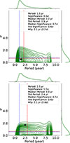 |
Fig. B.1. Top: Distributions for the period and significance for the simulated light curves with the same properties as the X-ray data using 100.000 artificial light curves with the same properties as the original light curve (i.e., sampling, gap distribution, PSD, PDF) for the method GLSP. The results denote that the period and significance obtained are compatible with random light curves with the same gap structure as the original X-ray light curve. Bottom: Distributions for the period and significance for the simulated light curves with the same properties as the 30-day binned X-ray data using 100.000 artificial light curves with the same properties as the original light curve (i.e., sampling, gap distribution, PSD, PDF) for the method GLSP. The results indicate that the period and significance recovered from the real data could, in principle, arise from the gap structure, but this scenario is unlikely in the case of the binned light curve. The dotted red vertical and horizontal lines indicate the median values for both the period and the significance of the test. The blue dotted vertical line highlights the most frequently occurring period in the tests (and the associated significance), emphasizing its prominence in the distribution. The “Median Period” represents the median of all periods resulting from the test, and the “Std Period” is the standard deviation of such periods’ distribution. The “Median Significance” represents the median of the significance distribution associated with the test, and the “Std Significance” is the standard deviation of this significance distribution. “Mfp” represents the most frequent period resulting from the test. |
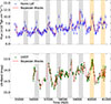 |
Fig. B.2. Bayesian blocks of the Fermi-LAT and UVOT (filter "uvv") light curves are shown. The gray vertical lines approximately mark the high-emission states corresponding to the inferred period of ≈2.1 years, while the orange vertical lines approximately indicate the Swift monitoring campaign carried out to track the predicted high states. The figure highlights the near-coincidence of the γ-ray high-emission phase with a similar state observed in UV. |
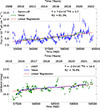 |
Fig. B.3. Trend decomposition. Top: γ ray. Bottom: UV (filter "uvv"). The green (blue) lines represent the underlying trend extracted by the function seasonal_decompose. Note that the green (blue) line covers a shorter time span than the full light curve duration, a result of the trend decomposition applied by this function. The red line indicates the fit of the green line, with the dashed red line extending the fitted line across the entire light curve. R2 is 81.3% and 76.8% for γ ray and UV, respectively, denoting a ”substantial” fit in both cases. |
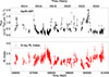 |
Fig. B.4. Representation of the X-ray flux and the power-law indices resulting from the fitting model. |
Appendix C: Discarded Swift observations
This section presents details and figures relating to discarded Swift observations in the analysis. The Swift-XRT analysis results only on the discarding of three observations, one of them due to bad coordinate association (OBSID 00046686005, see Fig. C.1), and two of them due to empty event files (OBSIDs 00019035008 and 00046686005).
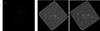 |
Fig. C.1. Examples of discarded Swift observations after a visual inspection of the FOV and the extraction (small) and background (large) regions. Left: Discarded XRT pc observation (OBSID 00046686005), due to incorrect coordinate association. Incidentally, the source is not detected in this observation, implying that the data would have been discarded at a later stage, when the fit would not have converged. Center and Right: Examples of discarded UVOT observations (OBSIDs 00031368135 and 00031368090, respectively), due to varying degrees of imperfect tracking. |
The Swift-UVOT analysis results in the removal of 28 observations, all of them due to varying degrees of bad tracking. Two examples, of different levels of tracking loss, are shown in Fig. C.1. The list of removed OBSIDs is as follows: 00031368072, 00031368090, 00031368129, 00031368135, 00031368137, 00031368177, 00031368181, 00031368247, 00035021014, 00035021016, 00035021021, 00035021073, 00035021074, 00035021085 00035021133, 00035021144, 00035021155, 00035021176, 00035021212, 00035021215, 00035021221, 00035021223, 00035021224, 00035021225, 00035021226, 00046686005, 00092186008, 00096880004.
All Tables
All Figures
|
Fig. 1. Multiwavelength light curves of PG 1553+113 used in this study. The vertical orange bands mark the approximate locations of the Swift monitoring campaigns that targeted the predicted high-emission states. Top: Fermi-LAT light curve (30-day binning). Center: Swift-XRT light curve, including both PC and WT observations. Bottom: UVOT UV band light curve (uvv filter). The analysis uses data from MJD ∼55 000 onward to avoid potential inconsistencies associated with the large data gap prior to that date (Peñil et al. 2025e). |
| In the text | |
|
Fig. 2. Bayesian blocks of Fermi-LAT and Swift-XRT light curves. The vertical gray lines approximately mark the high-emission states corresponding to the inferred period of ≈2.1 years, while the vertical orange lines approximately indicate the Swift monitoring campaign designed t to track the predicted high states. |
| In the text | |
|
Fig. 3. Trend decomposition of the X-ray data. The green line shows the underlying trend extracted using seasonal_decompose. The trend covers a shorter time span than the full light curve duration because of decomposition method. The red line shows the fit to this trend; the dashed red line extends the fit line across the full light curve. The R2 value is 77.2%, indicating a good fit. |
| In the text | |
|
Fig. 4. Bayesian blocks of the X-ray flux and the power-law index from the fitting model. An apparent anti-correlation is visible between the flux and the associated PL index. The vertical gray lines mark the high-emission states corresponding to the inferred period of ≈2.1 years, while the vertical orange lines indicate the Swift monitoring campaign designed to track the predicted high states. |
| In the text | |
|
Fig. B.1. Top: Distributions for the period and significance for the simulated light curves with the same properties as the X-ray data using 100.000 artificial light curves with the same properties as the original light curve (i.e., sampling, gap distribution, PSD, PDF) for the method GLSP. The results denote that the period and significance obtained are compatible with random light curves with the same gap structure as the original X-ray light curve. Bottom: Distributions for the period and significance for the simulated light curves with the same properties as the 30-day binned X-ray data using 100.000 artificial light curves with the same properties as the original light curve (i.e., sampling, gap distribution, PSD, PDF) for the method GLSP. The results indicate that the period and significance recovered from the real data could, in principle, arise from the gap structure, but this scenario is unlikely in the case of the binned light curve. The dotted red vertical and horizontal lines indicate the median values for both the period and the significance of the test. The blue dotted vertical line highlights the most frequently occurring period in the tests (and the associated significance), emphasizing its prominence in the distribution. The “Median Period” represents the median of all periods resulting from the test, and the “Std Period” is the standard deviation of such periods’ distribution. The “Median Significance” represents the median of the significance distribution associated with the test, and the “Std Significance” is the standard deviation of this significance distribution. “Mfp” represents the most frequent period resulting from the test. |
| In the text | |
|
Fig. B.2. Bayesian blocks of the Fermi-LAT and UVOT (filter "uvv") light curves are shown. The gray vertical lines approximately mark the high-emission states corresponding to the inferred period of ≈2.1 years, while the orange vertical lines approximately indicate the Swift monitoring campaign carried out to track the predicted high states. The figure highlights the near-coincidence of the γ-ray high-emission phase with a similar state observed in UV. |
| In the text | |
|
Fig. B.3. Trend decomposition. Top: γ ray. Bottom: UV (filter "uvv"). The green (blue) lines represent the underlying trend extracted by the function seasonal_decompose. Note that the green (blue) line covers a shorter time span than the full light curve duration, a result of the trend decomposition applied by this function. The red line indicates the fit of the green line, with the dashed red line extending the fitted line across the entire light curve. R2 is 81.3% and 76.8% for γ ray and UV, respectively, denoting a ”substantial” fit in both cases. |
| In the text | |
|
Fig. B.4. Representation of the X-ray flux and the power-law indices resulting from the fitting model. |
| In the text | |
|
Fig. C.1. Examples of discarded Swift observations after a visual inspection of the FOV and the extraction (small) and background (large) regions. Left: Discarded XRT pc observation (OBSID 00046686005), due to incorrect coordinate association. Incidentally, the source is not detected in this observation, implying that the data would have been discarded at a later stage, when the fit would not have converged. Center and Right: Examples of discarded UVOT observations (OBSIDs 00031368135 and 00031368090, respectively), due to varying degrees of imperfect tracking. |
| In the text | |
Current usage metrics show cumulative count of Article Views (full-text article views including HTML views, PDF and ePub downloads, according to the available data) and Abstracts Views on Vision4Press platform.
Data correspond to usage on the plateform after 2015. The current usage metrics is available 48-96 hours after online publication and is updated daily on week days.
Initial download of the metrics may take a while.