| Issue |
A&A
Volume 686, June 2024
|
|
|---|---|---|
| Article Number | A300 | |
| Number of page(s) | 7 | |
| Section | Extragalactic astronomy | |
| DOI | https://doi.org/10.1051/0004-6361/202449515 | |
| Published online | 21 June 2024 | |
Unveiling the periodic variability patterns of the X-ray emission from the blazar PG 1553+113
1
INAF – Osservatorio Astronomico di Roma, Via Frascati 33, 00078 Monte Porzio Catone, RM, Italy
e-mail: This email address is being protected from spambots. You need JavaScript enabled to view it.
2
“Sapienza” Università di Roma – Dip. di Fisica, P.le A. Moro 5, 00185 Roma, Italy
3
Università degli Studi di Roma “Tor Vergata” – Dip. di Fisica, Via della Ricerca Scientifica 1, 00133 Roma, Italy
4
INFN – Roma Tor Vergata, Via della Ricerca Scientifica 1, 00133 Roma, Italy
5
University of Maryland – Dept. of Astronomy, College Park, MD 20742, USA
6
NASA – Goddard Space Flight Center, Greenbelt Rd. 8800, Greenbelt, MD 20771, USA
7
ASI – Space Science Data Center, Via del Politecnico snc, 00133 Roma, Italy
8
Scuola Normale Superiore di Pisa, P.zza dei Cavalieri 7, 56126 Pisa, Italy
Received:
6
February
2024
Accepted:
5
April
2024
Abstract
The search for periodicity in the multiwavelength, highly variable emission of blazars is a key feature to understanding dynamical processes at work in this class of active galactic nuclei. The blazar PG 1553+113 is an attractive target due to the evidence of periodic oscillations observed at different wavelengths, with a solid proof of a 2.2-year modulation detected in the γ-ray, UV, and optical bands. We aim to investigate the variability pattern of the PG 1553+113 X-ray emission using a more than 10-year-long light curve in order to robustly assess the presence or lack of a periodic behavior, evidence of which is only marginal so far. We conducted detailed statistical analyses, studying in particular the variability properties of the X-ray emission of PG 1553+113 by computing the Lomb-Scargle periodograms, which are suited for the analyses of unevenly sampled time series, and adopting epoch-folding techniques. We find a modulation pattern in the X-ray light curve of PG 1553+113 with a period of ∼1.4 years, which is about 35% shorter than the one observed in the γ-ray domain. Our finding is in agreement with the recent spectro-polarimetric analyses and supports the presence of more dynamical phenomena simultaneously at work in the central engine of this quasar.
Key words: black hole physics / galaxies: active / BL Lacertae objects: general / BL Lacertae objects: individual: PG 1553+113 / X-rays: galaxies / X-rays: general
© The Authors 2024
 Open Access article, published by EDP Sciences, under the terms of the Creative Commons Attribution License (https://creativecommons.org/licenses/by/4.0), which permits unrestricted use, distribution, and reproduction in any medium, provided the original work is properly cited.
This article is published in open access under the Subscribe to Open model. This email address is being protected from spambots. You need JavaScript enabled to view it. to support open access publication.
1. Introduction
Blazars are a class of active galactic nuclei (AGN) characterized by extreme luminosity and variability over the entire electromagnetic spectrum. Their emission is dominated by a single component, that is a jet of relativistic particles directly pointing toward the observer (Urry & Padovani 1995). From a spectroscopic point of view, these sources show a peculiar spectral energy distribution (SED) that is characterized by a double-humped shape. The low-frequency peak, which can be observed from the radio up to the X-ray domain, is attributed to synchrotron radiation arising from high-energy electrons that spiral around magnetic field lines (Padovani & Giommi 1995); its properties mainly depend on the strength of the magnetic field and on the energy distribution of the relativistic electrons in the jet (Maraschi et al. 1992). The second hump is usually observed in the X-to-γ-ray range, and its origin is commonly associated with inverse Compton (IC) emission (Ghisellini et al. 1992; Abdo et al. 2011; Zdziarski & Bottcher 2015) or synchotron self-Compton, where the seed photons emerge from either external radiation fields (external Compton; EC) or the synchrotron radiation of the jet itself, respectively. Much evidence – from SED modeling (e.g., Abdo et al. 2011) and energetic considerations (Zdziarski & Bottcher 2015; Liodakis & Petropoulou 2020) to observations of correlated flux variations across different wavebands (e.g., Agudo et al. 2011a,b; Liodakis et al. 2018), and, recently, polarimetry (Middei et al. 2023a; Peirson et al. 2023) – supports the leptonic origin of the second hump of the blazars SED.
A hallmark of the blazar phenomenon is the prominent flux and spectral variability, which is thought to arise from changes in the jet properties such its particle density, magnetic field strength, and orientation (Padovani & Giommi 1995). Variability can be observed over different timescales from hours up to decades (Kellermann 1992). In this context, the search for periodic signals is increasingly attracting attention, and the high synchrotron-peaked source PG 1553+113 represents one of the most interesting cases. PG 1553+113, a blazar with optical magnitude V ∼ 14.5 at redshift z ∼ 0.4 − 0.5 (Danforth et al. 2010), shows evidence of a periodicity (T ∼ 2.2 yr) in the γ-ray band (E ≥ 100 MeV) sampled by the Fermi-LAT satellite and at lower frequencies (R-band; Ackermann et al. 2015; Sobacchi et al. 2017; Peñil et al. 2024). A possible explanation for the periodic signal was proposed by Sobacchi et al. (2017), who discussed a scenario where a couple of asymmetric super massive black holes (SMBHs), of which the smallest carries a jet, interacts and produces a precession of the jet itself.
The temporal properties of the PG 1553+113 X-ray emission are instead more debated. Huang et al. (2021) claimed the finding of the same periodicity with respect to the γ-ray emission within a scenario in which both SMBHs possess a jet. Conversely, Peñil et al. (2024), working on a blazar sample, identified a periodicity of ∼1.5 years with a significance level of ∼2σ. In this paper, we report on the temporal properties of PG 1553+113 by investigating the data collected in the rich Swift archive, which provides 617 X-ray and > 400 optical-UV observations. By constructing the source multiwavelength (MWL) light curves (LCs), we correlated the various emission bands and searched for an unambiguous periodic signal at each wavelength with robust methods of time-series analysis, such as the construction of the Lomb-Scargle periodograms (Lomb 1976; Scargle 1982) and the application of epoch folding techniques (e.g., Larsson 1996), with particular attention paid to the X-ray signal in order to identify an associated periodicity with adequate significance.
The paper is organized as follows. In Sect. 2, we illustrate the data selection and reduction; in Sect. 3, we compute correlations between different bands; in Sect. 4, we present the X-ray variability analysis; in Sect. 6, we discuss our findings; finally, in Sect. 7, we summarize the obtained results. Throughout the text, we adopt a concordance cosmology with H0 = 70 km s−1 Mpc−1, ΩM = 0.3, and ΩΛ = 0.7.
2. Observations and data reduction
Launched in 2004, the Swift satellite carries the X-ray Telescope (XRT), which is sensitive in the 0.2 − 10 keV energy band, and the UV-Optical Telescope (UVOT), capable of observations in the 170 − 600 nm band. the XRT has high spatial resolution of 18″, allowing for precise localization of celestial objects. The XRT and UVOT operate simultaneously to enable concurrent observations in different electromagnetic bands (Roming et al. 2005; Burrows et al. 2005). We retrieved the X-ray, UV and optical reduced data from 2005 to 2023 from the Swift public mirror archive1 of the Space Science Data Center (SSDC) at the Italian Space Agency (ASI). In this analysis, we excluded the data taken before 2012, characterized by a sparse temporal sampling, to avoid the introduction of biases that could be ascribed to time intervals containing no data points.
The Swift-XRT observations were carried out in the windowed-timing (WT) and photon-counting (PC) readout modes. The data were first reprocessed locally with the XRTDAS software package (version v3.7.0), developed by the ASI-SSDC and included in the NASA-HEASARC HEASoft package2 (version v6.31.1). Standard calibration and filtering processing steps were applied to the data using the xrtpipeline task. The calibration files available from the Swift-XRT CALDB (version 20220803) were used. Events for the temporal and spectral analysis were selected within a circle of a 20-pixel (∼47″) radius, while the background was estimated from nearby circular regions with a radius of 40 pixels. For each observation, the X-ray energy spectrum was first binned with the grppha tool of the FTOOLS package3 to ensure a minimum of 20 counts per bin and then modeled using the XSPEC software package4 adopting a single power-law model.
We obtained dereddened UV and optical fluxes with a dedicated ASI-SSDC pipeline for the analysis of UVOT sky images (Giommi et al. 2012). We first executed the aperture photometry task included in the UVOT official software from the HEASoft package (version v6.26), extracting source counts within a standard 5″ circular aperture and the background counts from three circular 18″ apertures that were selected to exclude nearby stars. We then derived the source dereddened fluxes by applying the official UVOT calibrations from the CALDB (Breeveld et al. 2011) and adopting a standard UV-optical mean interstellar extinction law (Fitzpatrick 1999) with a mean E(B − V) value of 0.0447 mag (Schlafly & Finkbeiner 2011). We show the X-ray, UV (M2 filter), and optical (B-band) LCs obtained in this way in Fig. 1, along with the X-ray photon index: a visual inspection already reveals considerable flux variability. Furthermore, while the UV and optical trends can be overlapped, the X-ray band exhibits some peaks that do not appear in the other bands, hinting at a possible X-ray periodicity that is different to the optical-UV one.
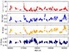 |
Fig. 1. MWL LCs of PG 1153+113 in B (yellow dots), M2 (blue dots), X-ray (red dots) bands, and spectral index (dark blue dots) from 2012 to 2023 of Swift satellite. The X-ray fluxes are in 0.2−10 keV band. B, M2, and X-ray’s LCs are shown along with the corresponding 1σ uncertainties. |
3. Correlations between different bands and between photon index and X-ray flux
We first proceeded studying the correlations among the various bands, and between X-ray photon index and flux. The photon index and the X-ray flux of PG 1553+113 in the 0.3−10 keV band are moderately anticorrelated (see Fig. 2) as we computed a Pearson coefficient (Bevington & Robinson 2003) of r = −0.55 and an associated null-hypothesis probability p(> r) = 3.6 × 10⁻²⁴ (see Table 1). The X-ray photon index is flatter as the source flux increases. This is commonly observed in blazars (the so-called “harder-when-brighter” behavior; e.g., Giommi et al. 2021) and is expected when particles are injected and accelerated in the jet (Abdo et al. 2010).
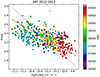 |
Fig. 2. PG 1553+113 X-ray photon index–to-flux correlation. The two linear fits of photon index versus flux and vice versa (red dotted lines) are shown along with the corresponding bisector fit (red dashed line). The data points are color-coded on the basis of their MJD. |
Results of the correlation analysis (Pearson correlation coefficients and number of degrees of freedom) between pairs of wavebands and between the X-ray photon index and flux.
We then tested the correlation properties between the UV, optical, and X-ray bands, respectively. Moderate correlations were found as shown in Fig. 3 and Table 1. Such a study highlights the typical behavior of the radiation emitted from blazars in adjacent wavebands such as the X-rays and the optical-UV, since the respective emitting regions are partially overlapping in the jet and produce photons through the same underlying physical process (i.e., the synchrotron or IC radiation) – or by processes that make it vary in a quasi-simultaneous way (Dhiman et al. 2021).
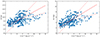 |
Fig. 3. Correlations of UV-to-X-ray and optical-to-X-ray bands of PG 1553+113. As in Fig. 2, the two linear correlation fits (red dotted lines) are shown along with the corresponding bisector fit (red dashed line). |
4. Multiwavelength variability analysis
To investigate the periodic behavior of the X-ray emission in PG 1553+113, we performed an analysis of the LC through the employment of numerical methods that are commonly used in studies of time series. In particular, we mainly relied on the construction of the Lomb–Scargle (LS) periodogram (Lomb 1976; Scargle 1982), a technique that is widely adopted to search for periodic signals in astronomical data sets (e.g., VanderPlas 2018; Vio et al. 2013) and especially suited for analyzing unevenly sampled time series (Baluev 2008). This method consists of the calculation of the power spectral density (PSD) of a time series and estimating the signal likelihood at each frequency on the basis of a least-squares fit of a sinusoidal model to the data. For our analysis, we adopted the LS routines contained inside the AstroPy (v5.0) Python package (Astropy Collaboration 2022).
In carrying on our analysis, we already knew that the optical (and the associated UV) LCs exhibit an ∼2.2-yr period (Sobacchi et al. 2017); therefore, we expected the calculation of the LS periodogram for such LCs to yield a comparable result as a confirmation of the goodness of the method. We thus computed the LS periodograms associated with the PG 1553+113 X-ray, UV, and optical LCs, and identified prominent peaks in the PSD. We show the results in the left panels of Fig. 4: a visual inspection reveals that, while the main peak associated with the optical and UV variability patterns is located at the same frequency, a clearly prominent peak also appears for the X-ray signal, but – at variance with the optical-UV case – it is shifted at a larger frequency (corresponding to a shorter period).
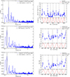 |
Fig. 4. LS periodograms associated with the corresponding MWL LCs of PG 1553+113. Left panels: PG 1553+113 LS periodograms of X-ray, UV (W2), and optical bands (V; blue solid lines). In each panel, the frequency of the main peak (black dashed line) is highlighted and its value is reported (see legend). Right panels: X-ray, UV, and optical LCs (blue points), along with the relative sinusoids of periods corresponding to the LS most significant frequencies (red dashed lines). In such panels, the sinusoid maxima approximately coinciding with flux peaks in the LCs (gray dot-dashed lines) are marked, and the corresponding period is reported (see legend). |
We found that such a peak was located at a frequency of ∼2.3 × 10⁻⁸ Hz, corresponding to TX ∼ 1.4 years. This value is significantly lower, by ∼35%, than the γ-ray period Tγ ∼ 2.2 years identified in the Fermi-LAT data by Ackermann et al. (2015) and in the optical LC by Sobacchi et al. (2017), thus hinting at the presence of a different periodic process. To quantify the significance of this peak, we estimated its false alarm probability (FAP) level, i.e. the probability of accidentally obtaining a given peak power due to noise fluctuations. We only considered peaks whose FAP level was falling below ∼10% (Sturrock & Scargle 2010) as statistically significant, setting the corresponding LS power of ∼0.04 as our 1σ significance level; in doing so, we obtained a significance level of 9.2σ for the 1.4-yr X-ray peak. We also repeated the procedure on the entire PG 1553+113 X-ray LC from 2005 to 2023 (i.e., including data that were discarded in the selection described in Sect. 2) to check the persistence of the peak in the LS periodogram. The test yielded the same TX with a significance of 7.5σ. We argue that this lower significance is due to the presence of large time gaps in the complete X-ray LC (see Fig. 1).
In the UV and optical LS periodograms, we found a frequency of the most significant peak of ∼1.5 × 10⁻⁸ Hz that corresponds to Topt ∼ 2.1 years with a significance of 5.8σ (see Fig. 4). For completeness, we also tested the LS analysis on the publicly available Fermi-LAT γ-ray data5 from 2008 to 2023. In doing so, we again obtained the peak at a frequency of ∼1.5 × 10⁻⁸ Hz with a significance level of 7.3σ, corresponding to the well-known Tγ ∼ 2.2 years found by Ackermann et al. (2015). Having retrieved a comparable result with that reported in the literature for the PG 1553+113 joint optical-γ-ray signal (Sobacchi et al. 2017), this analysis strengthens our finding of a discrepant TX with respect to the variability period of the LCs in other wavebands.
To further confirm the temporal properties of the PG 1553+113 X-ray emission, we applied two different methods. First, we used the timing tasks provided by the Xronos software package6, designed for the analysis of high-energy astrophysical data (Stella & Angelini 1992). We started from the power-spectrum (powerspec) method to calculate the PSD of the LCs in each energy band; in this way, we identified the significant peaks corresponding to potential periods in the X-ray LC that match the results obtained with the LS analysis. Then, we applied the epoch-folding search (efsearch) method to perform the calculation of the posterior distribution of the LC periodicities. The distribution peak yielded a best-fit period of ∼1.4 years, further confirming the LS findings. Finally, we employed the epoch-folding (efold) method to generate folded LCs at the specific periods of interest. We show the outcome of this cross-check in Fig. 5.
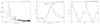 |
Fig. 5. Analysis results obtained with the Xronos software. Left panel: PG 1553+113 PSD of X-ray LC obtained with the powerspec package of Xronos. Middle panel: best-fit period (solid line) of PG 1553+113 X-ray LC obtained with the efsearch task, along with its numerical value in seconds corresponding to ∼1.4 years (see text). Right panel: epoch folding of PG 1553+113 X-ray LC obtained with the efold method on the basis of the best-fit period determined by efsearch. |
We also used the “significance-spectrum” (SigSpec) algorithm developed for asteroseismology (Reegen 2007; Chang et al. 2011; Maceroni et al. 2014), which is based on the analysis of frequency- and phase-dependent spectral significance levels S of peaks in a discrete Fourier transform of the signal, through the computation of the probability density function and its associated FAP due to white noise. As the LS analysis, this method is particularly suited for periodicity studies on sparse data. We thus executed the SigSpec algorithm on the UVOT W2 and V time series and finally on the X-ray time series, obtaining the highest significance periods of TW2 ∼ 2.08 years (SW2 ∼ 28.0), TV ∼ 2.11 years (SV ∼ 29.6), and PX ∼ 1.39 years (SX ∼ 27.5), respectively. Also, such values are in agreement with those obtained with the LS, thus confirming the goodness of our result.
5. X-ray period uncertainty estimate and red-noise bias analysis
The calculation of the LS periodogram does not provide any estimate of the uncertainty on the position of the significant peaks. To estimate this quantity, we performed an extensive LS analysis over many altered versions of the PG 1553+113 X-ray LC, in which we replaced each point with a new observing epoch and flux level that differ from the original ones by random amounts extracted from appropriate distributions centered on the actual data. For altering the observing epochs, we adopted uniform distributions, with widths equal to the full width at half maximum (FWHM) of ∼1 year derived from the Gaussian fit to the distribution of best-fit periods computed by the efsearch task (see Fig. 5); for the flux values, we instead adopted Gaussian distributions with standard deviations equal to the associated 1σ errors. In this way, we produced 103 realizations of the PG 1553+113 X-ray LC; for each realization, we then computed the LS periodogram and derived the posterior distribution of frequencies of the most significant peak. The statistical analysis of this distribution yielded a best estimate of the PG 1553+113 X-ray period of TX = 1.41 ± 0.68 years.
Despite the high significance level of our results, we are unable to automatically exclude that the LS analysis is biased by sources of uncertainty that could produce fake signals in the periodogram. This could be due to nonperiodic processes that can mimic a periodic temporal behavior on the timescales of our interest, such as random variability in the AGN flux that is usually distributed according to a red-noise spectrum (Bhatta 2017; Vaughan et al. 2016). Since the PSD of blazar LCs is of the red-noise type (Vaughan 2005), the power level – and thus the FAP – is expected to increase at low frequencies. To assess that our results are not biased by red-noise processes, we simulated the response of the LS analysis to a sample of mock LCs generated according to a pure red-noise PSD.
To this aim, we generated such LCs by extracting, from a red-noise spectral distribution (e.g., Gardiner 1994), a number of fake flux points corresponding to the amount of X-ray data at our disposal, and we associated each of them with an MJD time of our observations. We iterated this process 105 times to reach the statistical significance of the results; for each mock LC produced in this way, we computed the associated LS periodogram using the same methodology described in Sect. 4. Requesting a minimum LS power of ∼0.04 as our 1σ level (i.e., the same amount associated with the threshold FAP of our real data; see Sect. 4), we found that at most ∼16% of our mock LCs rise above 5σ in the frequency range of interest, (2 − 3)×10−8 Hz (see Fig. 6). Such a fraction is non-negligible, and thus suggests some caution should be taken in claiming a firm discovery of the ∼1.4-year periodicity; nevertheless, these findings point toward the plausible detection of a true periodic signal in the X-ray LC of PG 1553+113 at an ∼84% confidence level.
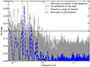 |
Fig. 6. LS periodograms calculated on randomly generated LCs of pure red noise. For plotting purposes, we show 102 (gray solid lines) out of the total 105 realizations, superimposed on the LS periodogram of the real PG 1553+113 X-ray data (blue dot-dashed line) and the corresponding 5σ significance level (black dashed line; see Sect. 4). The relevant frequency interval for our analysis of (2 − 3)×10−8 Hz (black dotted lines) is also highlighted. |
6. Discussion
The presence of multiple periodic patterns in the MWL LCs of PG 1553+113 has been the subject of various studies (Ackermann et al. 2015; Sobacchi et al. 2017; Huang et al. 2021; Peñil et al. 2022; Adhikari et al. 2024); recently, there has also been the indication of a potential long-term variability trend in the γ-ray emission (∼22 years; Adhikari et al. 2024; Peñil et al. 2024). Different scenarios have been proposed to explain this behavior. The most widely accepted one relies upon the presence, inside the PG 1553+113 central engine, of a binary system of SMBHs in which one of the two carries a jet that is gravitationally affected by the SMBH motions (Ackermann et al. 2015). This may happen in several ways, such as (i) a jet precession (Sobacchi et al. 2017), (ii) a helical shaping of the jet (Abdo et al. 2010), or (iii) instabilities in the jet structure (Huang et al. 2021). Alternatively, (iv) accretion modulations (Tavani et al. 2018) and (v) evaporation processes possibly coexisting with disk overdensities (Adhikari et al. 2024) may also lead to similar results.
The γ-ray and optical period was already modeled by Sobacchi et al. (2017), considering a jet precession with a period of Tγ ∼ 2.2 years. To account for an overall different X-ray period, Huang et al. (2021) fit the Swift-XRT LC with a two-jet model, each carried by one of the PG 1553+113 SMBHs, assuming a precession with TX ∼ 2.2 years acting on both jets; however, their result is based on the analysis of a less extended X-ray LC with respect to ours. Also Peñil et al. (2024), by analyzing the Swift-XRT data of a sample of γ-ray detected blazars, found for PG 1553+113 an X-ray period of ∼1.5 years with a significance level of ∼2σ after averaging on the temporal properties of the entire sample.
A possible explanation that does not take into account a binary SMBH system could be the cyclic injection of large quantities of matter from the innermost regions of the central engine into the jet base (Lewis et al. 2019). If this input of matter occurs regularly, this could produce the emission of a modulated X-ray signal with a different period with respect to that of the γ-ray, UV, and optical emission (due to the jet precession). It is interesting to note that recent observations from the IXPE satellite (Middei et al. 2023b) indicate the presence of different emitting regions in the jet structure, hinting at either a stratified jet or different levels of turbulence inside the jet structure.
The plausible detection of a different time modulation of the PG 1553+113 X-ray emission with respect to the γ-ray, UV, and optical ones has further complicated the road to understanding the physical mechanisms acting in the central engine of this blazar. Future MWL observations and studies involving a more detailed modeling of the PG 1553+113 innermost structure (SMBH system, accretion disk, jet, and the respective interplay) will be crucial to eventually explaining the origin of its temporal properties.
7. Summary and future work
In this study, we conducted a comprehensive analysis of the X-ray, UV, and optical data of the blazar PG 1553+113, aimed at investigating the possible presence of a characteristic X-ray periodicity that differs from the already ascertained γ-ray and optical variability period. We summarize our main findings below.
-
The PG 1553+113 X-ray, UV, and optical LCs are all moderately correlated to each other according to the Pearson analysis (r ∼ 0.5); the X-ray photon index is correlated with the X-ray flux in a similar way. This behavior is typical of blazars, where the light is emitted almost entirely from the jet due to the synchrotron and IC processes (Padovani & Giommi 1995; Maraschi et al. 1992).
-
The X-ray LC constructed over ≳10 observer-frame years of Swift-XRT data likely (> 80% confidence level) exhibits a periodic emission, but with a shorter characteristic period of TX ∼ 1.4 years with respect to that found in the optical and γ-ray bands (Topt = TUV = Tγ ∼ 2.2 years; Ackermann et al. 2015; Sobacchi et al. 2017; Peñil et al. 2024).
Current scenarios are not able to properly explain such a difference in the widely accepted framework of a binary system of SMBHs carrying a preceding jet in the PG 1553+113 central engine (Huang et al. 2021; Tavani et al. 2018; Sobacchi et al. 2017; Adhikari et al. 2024). Therefore, further theoretical investigations and observational data are needed to better disentangle the physical mechanisms that lie at the base of the different variability periods of the PG 1553+113 MWL emission.
Available at https://swift.ssdc.asi.it/
Available at https://heasarc.gsfc.nasa.gov/docs/software/heasoft/
Available at https://heasarc.gsfc.nasa.gov/ftools/
Available at https://heasarc.gsfc.nasa.gov/xanadu/xspec/
Available at https://fermi.gsfc.nasa.gov/ssc/data/access/
Available at https://heasarc.gsfc.nasa.gov/xanadu/xronos/xronos.html
Acknowledgments
We thank the anonymous referee for their helpful comments. We acknowledge M. Imbrogno (INAF-OAR) for useful discussion about the use of the Xronos software. This article is part of TA’s work for the PhD in Astronomy, Astrophysics and Space Science, jointly organized by the “Sapienza” University of Rome, University of Rome “Tor Vergata” and INAF.
References
- Abdo, A. A., Ackermann, M., Ajello, M., et al. 2010, ApJS, 188, 405 [NASA ADS] [CrossRef] [Google Scholar]
- Abdo, A. A., Ackermann, M., Ajello, M., et al. 2011, ApJ, 730, 101 [NASA ADS] [CrossRef] [Google Scholar]
- Ackermann, M., Ajello, M., Albert, A., et al. 2015, ApJ, 813, L41 [NASA ADS] [CrossRef] [Google Scholar]
- Adhikari, S., Penil, P., Westernacher-Schneider, J. R., et al. 2024, ApJ, 965, 124 [CrossRef] [Google Scholar]
- Agudo, I., Marscher, A. P., Jorstad, S. G., et al. 2011a, ApJ, 735, L10 [NASA ADS] [CrossRef] [Google Scholar]
- Agudo, I., Jorstad, S. G., Marscher, A. P., et al. 2011b, ApJ, 726, L13 [NASA ADS] [CrossRef] [Google Scholar]
- Astropy Collaboration (Price-Whelan, A. M., et al.) 2022, ApJ, 935, 167 [NASA ADS] [CrossRef] [Google Scholar]
- Baluev, R. V. 2008, MNRAS, 385, 1279 [Google Scholar]
- Bevington, P. R., & Robinson, D. K. 2003, Data Reduction and Error Analysis for the Physical Sciences (Boston: McGraw-Hill) [Google Scholar]
- Bhatta, G. 2017, ApJ, 847, 7 [NASA ADS] [CrossRef] [Google Scholar]
- Breeveld, A. A., Landsman, W., Holland, S. T., et al. 2011, AIP Conf. Ser., 1358, 373 [Google Scholar]
- Burrows, D. N., Hill, J. E., Nousek, J. A., et al. 2005, Space Sci. Rev., 120, 165 [Google Scholar]
- Chang, D. C., Ngeow, C. C., & Chen, W. P. 2011, in 9th Pacific Rim Conference on Stellar Astrophysics, eds. S. Qain, K. Leung, L. Zhu, & S. Kwok, ASP Conf. Ser., 451, 143 [Google Scholar]
- Danforth, C. W., Keeney, B. A., Stocke, J. T., Shull, J. M., & Yao, Y. 2010, ApJ, 720, 976 [NASA ADS] [CrossRef] [Google Scholar]
- Dhiman, V., Gupta, A. C., Gaur, H., & Wiita, P. J. 2021, MNRAS, 506, 1198 [NASA ADS] [CrossRef] [Google Scholar]
- Fitzpatrick, E. L. 1999, PASP, 111, 63 [Google Scholar]
- Gardiner, C. W. 1994, Handbook of Stochastic Methods for Physics, Chemistry and the Natural Sciences (Berlin: Springer) [Google Scholar]
- Ghisellini, G., Padovani, P., Celotti, A., & Maraschi, L. 1992, in Testing the AGN Paradigm, eds. S. S. Holt, S. G. Neff, & C. M. Urry, AIP Conf. Ser., 254, 398 [NASA ADS] [CrossRef] [Google Scholar]
- Giommi, P., Polenta, G., Lähteenmäki, A., et al. 2012, A&A, 541, A160 [NASA ADS] [CrossRef] [EDP Sciences] [Google Scholar]
- Giommi, P., Perri, M., Capalbi, M., et al. 2021, MNRAS, 507, 5690 [NASA ADS] [CrossRef] [Google Scholar]
- Huang, S., Yin, H., Hu, S., et al. 2021, ApJ, 922, 222 [NASA ADS] [CrossRef] [Google Scholar]
- Kellermann, K. I. 1992, Science, 258, 145 [NASA ADS] [CrossRef] [Google Scholar]
- Larsson, S. 1996, A&AS, 117, 197 [NASA ADS] [CrossRef] [EDP Sciences] [Google Scholar]
- Lewis, T. R., Finke, J. D., & Becker, P. A. 2019, ApJ, 884, 116 [NASA ADS] [CrossRef] [Google Scholar]
- Liodakis, I., & Petropoulou, M. 2020, ApJ, 893, L20 [Google Scholar]
- Liodakis, I., Romani, R. W., Filippenko, A. V., et al. 2018, MNRAS, 480, 5517 [NASA ADS] [CrossRef] [Google Scholar]
- Lomb, N. R. 1976, Ap&SS, 39, 447 [Google Scholar]
- Maceroni, C., Lehmann, H., da Silva, R., et al. 2014, A&A, 563, A59 [NASA ADS] [CrossRef] [EDP Sciences] [Google Scholar]
- Maraschi, L., Celotti, A., & Ghisellini, G. 1992, in Physics of Active Galactic Nuclei, eds. W. J. Duschl, & S. J. Wagner, 605 [CrossRef] [Google Scholar]
- Middei, R., Liodakis, I., Perri, M., et al. 2023a, ApJ, 942, L10 [NASA ADS] [CrossRef] [Google Scholar]
- Middei, R., Perri, M., Puccetti, S., et al. 2023b, ApJ, 953, L28 [NASA ADS] [CrossRef] [Google Scholar]
- Padovani, P., & Giommi, P. 1995, MNRAS, 277, 1477 [NASA ADS] [CrossRef] [Google Scholar]
- Peñil, P., Ajello, M., Buson, S., et al. 2022, arXiv e-prints [arXiv:2211.01894] [Google Scholar]
- Peñil, P., Westernacher-Schneider, J. R., Ajello, M., et al. 2024, MNRAS, 527, 10168 [Google Scholar]
- Peirson, A. L., Negro, M., Liodakis, I., et al. 2023, ApJ, 948, L25 [NASA ADS] [CrossRef] [Google Scholar]
- Reegen, P. 2007, A&A, 467, 1353 [NASA ADS] [CrossRef] [EDP Sciences] [Google Scholar]
- Roming, P. W. A., Kennedy, T. E., Mason, K. O., et al. 2005, Space Sci. Rev., 120, 95 [Google Scholar]
- Scargle, J. D. 1982, ApJ, 263, 835 [Google Scholar]
- Schlafly, E. F., & Finkbeiner, D. P. 2011, ApJ, 737, 103 [Google Scholar]
- Sobacchi, E., Sormani, M. C., & Stamerra, A. 2017, MNRAS, 465, 161 [NASA ADS] [CrossRef] [Google Scholar]
- Stella, L., & Angelini, L. 1992, XRONOS, A Timing Analysis Software Package: User’s Guide: Version 3.00 (Noordwijk: ESA Publications Division) [Google Scholar]
- Sturrock, P. A., & Scargle, J. D. 2010, ApJ, 718, 527 [NASA ADS] [CrossRef] [Google Scholar]
- Tavani, M., Cavaliere, A., Munar-Adrover, P., & Argan, A. 2018, ApJ, 854, 11 [NASA ADS] [CrossRef] [Google Scholar]
- Urry, C. M., & Padovani, P. 1995, PASP, 107, 803 [NASA ADS] [CrossRef] [Google Scholar]
- VanderPlas, J. T. 2018, ApJS, 236, 16 [Google Scholar]
- Vaughan, S. 2005, A&A, 431, 391 [NASA ADS] [CrossRef] [EDP Sciences] [Google Scholar]
- Vaughan, S., Uttley, P., Markowitz, A. G., et al. 2016, MNRAS, 461, 3145 [Google Scholar]
- Vio, R., Diaz-Trigo, M., & Andreani, P. 2013, Astron. Comput., 1, 5 [NASA ADS] [CrossRef] [Google Scholar]
- Zdziarski, A. A., & Bottcher, M. 2015, MNRAS, 450, L21 [NASA ADS] [CrossRef] [Google Scholar]
All Tables
Results of the correlation analysis (Pearson correlation coefficients and number of degrees of freedom) between pairs of wavebands and between the X-ray photon index and flux.
All Figures
|
Fig. 1. MWL LCs of PG 1153+113 in B (yellow dots), M2 (blue dots), X-ray (red dots) bands, and spectral index (dark blue dots) from 2012 to 2023 of Swift satellite. The X-ray fluxes are in 0.2−10 keV band. B, M2, and X-ray’s LCs are shown along with the corresponding 1σ uncertainties. |
| In the text | |
|
Fig. 2. PG 1553+113 X-ray photon index–to-flux correlation. The two linear fits of photon index versus flux and vice versa (red dotted lines) are shown along with the corresponding bisector fit (red dashed line). The data points are color-coded on the basis of their MJD. |
| In the text | |
|
Fig. 3. Correlations of UV-to-X-ray and optical-to-X-ray bands of PG 1553+113. As in Fig. 2, the two linear correlation fits (red dotted lines) are shown along with the corresponding bisector fit (red dashed line). |
| In the text | |
|
Fig. 4. LS periodograms associated with the corresponding MWL LCs of PG 1553+113. Left panels: PG 1553+113 LS periodograms of X-ray, UV (W2), and optical bands (V; blue solid lines). In each panel, the frequency of the main peak (black dashed line) is highlighted and its value is reported (see legend). Right panels: X-ray, UV, and optical LCs (blue points), along with the relative sinusoids of periods corresponding to the LS most significant frequencies (red dashed lines). In such panels, the sinusoid maxima approximately coinciding with flux peaks in the LCs (gray dot-dashed lines) are marked, and the corresponding period is reported (see legend). |
| In the text | |
|
Fig. 5. Analysis results obtained with the Xronos software. Left panel: PG 1553+113 PSD of X-ray LC obtained with the powerspec package of Xronos. Middle panel: best-fit period (solid line) of PG 1553+113 X-ray LC obtained with the efsearch task, along with its numerical value in seconds corresponding to ∼1.4 years (see text). Right panel: epoch folding of PG 1553+113 X-ray LC obtained with the efold method on the basis of the best-fit period determined by efsearch. |
| In the text | |
|
Fig. 6. LS periodograms calculated on randomly generated LCs of pure red noise. For plotting purposes, we show 102 (gray solid lines) out of the total 105 realizations, superimposed on the LS periodogram of the real PG 1553+113 X-ray data (blue dot-dashed line) and the corresponding 5σ significance level (black dashed line; see Sect. 4). The relevant frequency interval for our analysis of (2 − 3)×10−8 Hz (black dotted lines) is also highlighted. |
| In the text | |
Current usage metrics show cumulative count of Article Views (full-text article views including HTML views, PDF and ePub downloads, according to the available data) and Abstracts Views on Vision4Press platform.
Data correspond to usage on the plateform after 2015. The current usage metrics is available 48-96 hours after online publication and is updated daily on week days.
Initial download of the metrics may take a while.