


| Issue |
A&A
Volume 710, June 2026
|
|
|---|---|---|
| Article Number | A263 | |
| Number of page(s) | 21 | |
| Section | Planets, planetary systems, and small bodies | |
| DOI | https://doi.org/10.1051/0004-6361/202659736 | |
| Published online | 19 June 2026 | |
Destructuring the disk of AB Aurigae: Dynamics and accretion
1
LIRA, Observatoire de Paris, Université PSL, CNRS, Sorbonne Université, Univ. Paris Diderot, Sorbonne Paris Cité, CY Cergy Paris Université,
5 place Jules Janssen,
92195
Meudon,
France
2
Laboratoire d’Astrophysique de Bordeaux, Université de Bordeaux,
CNRS, B18N, Allée Geoffroy Saint-Hilaire,
33615
Pessac,
France
3
Academia Sinica, Institute of Astronomy and Astrophysics,
11F of AS/NTU Astronomy-Mathematics Building, No.1, Sec. 4, Roosevelt Rd,
Taipei,
Taiwan
4
Laboratoire CEA, IRFU/DAp, AIM, Université Paris-Saclay, Université Paris Diderot, Sorbonne Paris Cité, CNRS,
91191
Gif-sur-Yvette,
France
5
Colgate University,
13 Oak Dr.,
Hamilton,
NY
13346,
USA
6
Centro de Astrobiología (CAB), CSIC-INTA, ESAC Campus,
Camino bajo del Castillo s/n,
28692
Madrid,
Spain
7
Konkoly Observatory, HUN-REN Research Centre for Astronomy and Earth Sciences, MTA Centre of Excellence,
Konkoly-Thege Miklós út 15-17,
1121
Budapest,
Hungary
8
CNRS, IPAG, Univ. Grenoble Alpes,
38000
Grenoble,
France
9
IRAM, 300 rue de la piscine, Domaine Universitaire,
38406
SaintMartin d’Hères,
France
10
NASA Goddard Space Flight Center, Astrophysics Division,
Greenbelt,
MD,
20771,
USA
11
Observatoire de la Côte d’Azur,
96 Bd de l’Observatoire,
06304
Nice,
France
12
Department of Astronomy, Xiamen University,
Xiamen,
China
13
IRAP, Université de Toulouse, CNRS, Université Paul Sabatier, CNES,
Toulouse,
France
14
Space Telescope Science Institute,
3700 San Martin Drive,
Baltimore,
MD,
21218,
USA
15
Centre de recherche astrophysique de Lyon (CRAL),
Université Claude Bernard Lyon 1, CNRS, ENS, 9 avenue Charles Andre,
69561
Saint Genis Laval,
France
16
European Southern Observatory,
Karl-Schwarzschild-Straße 2,
85748
Garching,
Germany
★ Corresponding author: This email address is being protected from spambots. You need JavaScript enabled to view it.
Received:
6
March
2026
Accepted:
27
April
2026
Abstract
Context. The young disk around AB Aur features a complex assembly of spiral arms, several compact structures, and a protoplanet candidate, AB Aur b, suggesting ongoing planet formation in this young system. Because of its brightness and spatial extent, AB Aur represents a perfect laboratory for investigating the conditions under which planets start to form around intermediate-mass stars.
Aims. In this paper, we present near-IR polarized images of the AB Aur disk at three epochs spanning 3.85 years with SPHERE/IRDIS, as well as Hα images obtained with SPHERE/ZIMPOL at a single epoch. The purpose of this study is to analyze the dynamics of the entire disk and of the various structures in near-IR polarimetry, and to identify sources of Hα emission to derive constraints on their mass accretion rate.
Methods. We developed a method to measure the rotation of the disk as a function of the radius, covering physical separations from as close as ~25 au up to 400 au. We applied this method to the global structure of the disk as well as to specific features of interest, including both extended or compact sources. For the compact sources, we performed orbital analyses. We also studied the variability of shadows seen as thin radial streaks. For the Hα data, we extracted photometric measurements of several features and derived estimations of the accretion luminosities and mass accretion rates, assuming three different accretion models.
Results. The dynamical study in the near-IR shows that the disk globally follows Keplerian rotation, but we observe a departure from this behavior at radii smaller than ~60 au. At the smallest radius of ~25 au, we measure a deviation from Keplerian rotation as large as ~12° over 3.85 years, demonstrating sub-Keplerian rotation. The two bright spirals within the millimeter cavity have different dynamic trends, and we discuss their possible link with the identified planet candidates. We also discuss the implications of the non-Keplerian behavior, and we posit that it could be related to interactions with multiple protoplanets orbiting out of the disk plane on elliptical orbits. Furthermore, the orbital analysis of the compact sources (labeled f1, f2, and f3) suggests that their orbital planes are significantly inclined with respect to the disk plane by several tens of degrees. The variability of the shadows suggests that they are produced by optically thick regions located within ~60 au. For the photometric analysis in Hα, we derive a flux of about 8.22 × 10⁻¹⁵ erg/s/cm2 for the entire feature f1, but only 6.46 × 10⁻¹⁶ erg/s/cm2 at the location of AB Aur b, consistent with non-detection. If f1 were a point source and the accretion remained constant for 1 Myr, it would correspond to ~5-20 Jupiter masses according to the magnetospheric accretion model or ~6-10 Jupiter masses according to the boundary layer accretion model. We further discuss the non-detection of Hα emission on AB Aur b. Finally, we discuss the binarity of the host star, in particular using Gaia measurements.
Conclusions. AB Aur is a rare system in which the morphology and dynamics can be studied at a very high level of detail, contrasting with the generic picture of a young planet-forming disk. The excellent image quality of SPHERE, both in the near-IR and in the visible, allows us to track the disk rotation with unprecedented precision thanks to the stability of the instrument across several years and to study localized Hα emissions in the disk. Overall, these observations strongly argue for an active and complex phase of planet formation in this system.
Key words: methods: observational / techniques: high angular resolution / protoplanetary disks / planet-disk interactions / stars: individual
Publisher note: The missing movie was published separately on 23 June 2026, and a note indicating its availability was added to the article in the Data availability section.
© The Authors 2026
 Open Access article, published by EDP Sciences, under the terms of the Creative Commons Attribution License (https://creativecommons.org/licenses/by/4.0), which permits unrestricted use, distribution, and reproduction in any medium, provided the original work is properly cited.
This article is published in open access under the Subscribe to Open model. This email address is being protected from spambots. You need JavaScript enabled to view it. to support open access publication.
1 Introduction
The mechanisms that lead to the formation of protoplanets in the first million years of a planetary system lack observational data that would allow robust constraints on models proposing various formation pathways. However, in these early evolutionary stages (<5 Myr) planets are still embedded in their parent protoplanetary disk and presumably are surrounded by their own circumplanetary material (Szulágyi et al. 2022). For this reason, previous attempts to detect protoplanets and their circumplanetary disks (CPDs) in the near-IR were significantly impacted by contamination of the circumstellar disk (CSD), which implies high levels of dust opacities.
Indeed, while planets reside in disk midplanes, direct imaging in the visible and near-IR detects mostly scattered light from the central star bouncing off dust grains in the upper layers of the disk. To overcome this issue, most searches with groundbased adaptive optics (AO) systems and high-contrast imagers have focused on transition disks with dust cavities. Cavities not only suggest the presence of planets or chains of planets carving the disk, but also guarantee a level of dust opacity which allows the detection of protoplanets orbiting in the disk midplane. This strategy has proven effective for the planets PDS 70b,c (Müller et al. 2018; Haffert et al. 2019), and more recently, WISPIT 2b (Van Capelleveen et al. 2025). Several other protoplanet candidates are still awaiting confirmation or remain debated because they are found inside complex disk structures or do not appear as unambiguous and reproducible point sources (Sallum et al. 2015; Wagner et al. 2019; Gratton et al. 2019; Currie et al. 2022). However, considering that disk morphology and dynamics are considerably influenced by the presence of planets, these systems are valuable for studying the conditions and environments in which planets form and for testing different planet formation scenarios.
In this context, due to its brightness and spatial extension, which make it an ideal target for high contrast imaging observations, AB Aurigae (AB Aur) stands as a unique system with strong potential for studying planet formation. It has been studied with the most advanced instruments at high spatial resolution and across a large spectral range, delivering observations that are sensitive to the properties of gas and dust. On the one hand, there is particular interest in analyzing the complex spiral structures in this disk, both in thermal emission at submillimeter wavelengths (Tang et al. 2012, 2017; Fuente et al. 2017) and in scattered light in the near-IR (Boccaletti et al. 2020; Jorquera et al. 2022; Dykes et al. 2024). On the other hand, identifying planetary-mass objects responsible for the disk structures is an active field of research, which has led to the detection of the protoplanet candidate AB Aur b (Currie et al. 2022).
One of the striking characteristics of the AB Aur disk is its morphology, which harbors many individual spiral arms that wind from north to west. Several types of spirals have been identified, including those originally imaged by Fukagawa et al. (2004), which lie outside the cavity defined by the submillimeter ring located at about 1 arcsec (or ~160 au), as measured in the dust continuum at 1.3 mm (Tang et al. 2017). Some of these spirals are clearly located outside the disk plane and trace material falling onto the disk (Tang et al. 2012; Speedie et al. 2025). In contrast, the spirals located inside the cavity have attracted more interest, as they may have been caused by gravitational disturbances resulting from the presence of orbiting companions. In that respect, Tang et al. (2017) propose two protoplanet candidates based on the morphology of the spirals observed for the very first time in the gas with ALMA, the Atacama Large Mil-limeter/submillimeter Array; one of these could be related to AB Aur b, later detected by Currie et al. (2022), while the closer one coincides with the feature f1 reported in Boccaletti et al. (2020). Dong et al. (2016) also proposed a planet candidate in a gap at about 0.5" eastward of the star using hydrodynamical simulations based on earlier scattered-light images (Hashimoto et al. 2011), but so far such an object has not been identified in observations with deeper contrast capabilities.
In the protoplanet phase the gas is assumed to accrete at free-fall velocity onto the central object, creating a shock at the photosphere that in turn produces emission in hydrogen lines, while the accretion geometry defines the flux of these lines (Marleau et al. 2022). The most popular is the Hα line, which has motivated the construction of dedicated instruments or observing modes, including dual-band imagers such as ZIMPOL (Schmid et al. 2018, Zurich IMaging POLarimeter,), VAMPIRES (Visible Aperture Masking Polarimetric Imager for Resolved Exoplanetary Structures, Norris et al. 2015), MagAOX (Magellan Adaptive Optics eXtreme, Males et al. 2024), as well as spectro-imagers such as MUSE (Multi Unit Spectroscopic Explorer, Bacon et al. 2010). Although several surveys have yielded null results (Cugno et al. 2019; Zurlo et al. 2020; Xie et al. 2020), a few objects show clear signatures of Hα emission, including PDS70b,c (Haffert et al. 2019), WISPIT2b (Close et al. 2025), and Delorme 1 b (Eriksson et al. 2020), while again many other Hα candidates remain debated. AB Aur b (Currie et al. 2022), detected both in the near-IR with CHARIS/SCExAO (Coronagraphic High Angular Resolution Imaging Spectrograph at Subaru Coronagraphic Extreme Adaptive Optics, Groff et al. 2017) and in Hα, falls into this category. In contrast to other objects, it is spatially extended, which is interpreted as scattered light scattered from the CSD of an embedded protoplanet. Its variability in Hα suggests that accretion is ongoing (Bowler et al. 2025). However, UV and optical observations with the Wield Field Planetary Camera 3 on the Hubble Space Telescope (HST/WFPC3) favor the case of a circumstellar structure (Zhou et al. 2022, 2023). Finally, Currie et al. (2025) obtained a spectrum of AB Aur b revealing an inverse P Cygni profile for the Hα line (blueshifted emission component, redshifted absorption component) which they interpret as material infall, so compatible with accretion onto a protoplanet.
The present study provides additional observations along two lines: the morphology and dynamics of the spiral structures and the accretion rate extracted from Hα observations. In Section 2 we describe the observations with the IR Dual-band Imager and Spectrograph (IRDIS) in SPHERE (Spectro-Polarimetric High-contrast Exoplanet REsearch) in near-IR polarimetry, including data reduction, disk dynamics and features, shadows, and a discussion. Section 3 presents the results of SPHERE/ZIMPOL observations in the Hα filters, including photometric measurements, accretion rates, and a discussion. Section 4 concludes this work.
2 SPHERE/IRDIS polarimetric imaging
2.1 Observations and data reduction
We observed ABAur (V=7.05, H=5.06, K=4.23) with SPHERE/IRDIS in polarimetry with the Differential Polarimetric Imaging mode (DPI,12.25 mas/pixel) using the BB_H filter at three epochs in 2019 (period 104), 2021-2022 (period 108), and 2023 (period 112), approximately every two years (see Table 1 for the Log). In the second epoch we also obtained data in two other filters : BB_J and BB_Ks. We used the pupil-tracking mode to optimize coronagraphic performance (the pupil is fixed with respect to the Lyot stop) and to minimize variations in pupil aberrations. The coronagraph for the shortest-wavelength filters, BB_J and BB_H, has a diameter of 185 mas, while it is slightly larger for BB_Ks (230 mas). It uses a combination with an apodizer in the pupil following the principle of the apodized pupil Lyot coronagraph Soummer (2005), and Guerri et al. (2011). In the DPI mode of IRDIS, data acquisition proceeds through several polarimetric cycles. A “QU” cycle corresponds to four rotations of the half-wave plate to switch the orientation of the polarization states, which allows reconstruction of the Stokes Q and U vectors from the two beams on the detector (0° and 45° to derive Q+ and Q−, and 22.5° and 67.5° to derive U+ and U−). We obtained several data sets with the Ks filter in P108, but here we present the one with the best quality.
We reduced the data with the publicly available software IRDAP1 (IRDIS Data reduction for Accurate Polarimetry, Holstein et al. 2020), which follows the procedure of Boer et al. (2020) and is adapted from Schmid et al. (2006) to reject the unpolarized stellar signal through double-differencing.
Instead of using the Q and U Stokes parameters, we calculated the azimuthal Stokes parameters Qφ and Uφ. In this convention, Qφ represents the polarized intensity and Uφ the noise in the approximation of single scattering events. However, the Uφ image (Fig. A.2) indicates that multiple scattering is certainly taking place in AB Aur’s disk. We assumed that this had no impact on disk dynamics, provided that we performed relative measurements.
SPHERE observation log.
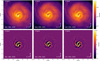 |
Fig. 1 H-band images of AB Aur Qφ in a 3″ × 3″ field of view at three epochs (December 2019, November 2021, and October 2023). The top row is displayed in logarithmic scale, while the bottom row is a high-pass filtered version in linear scale. The color bar shows the contrast obtained by normalizing with the out-of-mask point spread function image. North is up and east is left. |
2.2 General description
Figure 1 presents the Qφ images for the three epochs in the H band, while Fig. A.1 shows the second epoch only (P108), in the three bands. The top rows are displayed on a logarithmic scale, and the bottom rows are spatially filtered versions on a linear scale (obtained by subtracting a blurred image using a boxcar method with a width of 12 pixels to perform high-pass filtering and enhance the finest disk structures). Figure 2 displays the spatially filtered image of epoch 3 (October 2023) multiplied by the square of the stellocentric distance (r2) for visualization purposes (at this stage the image is not deprojected, so the r2 multiplication does not rigorously represent the density variation).
While the disk appears continuous in the submillimeter, it is more structured in the near-IR. To provide a synthetic view of the system, Fig. 2 (bottom panel) overlays the SPHERE image with the main components observed with ALMA: the “millimeter” ring (Tang et al. 2012), the CO inner spirals (Tang et al. 2017), the CO and SO rings (Dutrey et al. 2024), and the out-of-plane infalling spirals or streamers (Speedie et al. 2025).
As already presented in Boccaletti et al. (2020), the most striking features in the SPHERE image are the inner spiral arms, labeled S1 (eastern spiral) and S2 (western spiral), and also the “bridge”, which extends to the west and links the inner region to S2 (see Fig. 2 for labels). At the smallest angular separations, the two spirals wrap around the coronagraphic mask, possibly indicating the presence of the outer edge of the innermost disk detected in the mid-IR (Di Folco et al. 2009). The regions between the spiral arms are relatively dark, especially in the west, reminiscent of the submillimetric dust continuum cavity and the contrast of the spiral arms in CO (Tang et al. 2017).
These spirals are rather clumpy, as seen in the spatially filtered images in Fig. 2, in particular with the brightest feature labeled f1, “the twist,” at the root of S1 (PA ~ 212°), as previously reported in Boccaletti et al. (2020). Zoom-in images in Fig. 3 highlight the evolution of the various features discussed below. From a twisted feature in 2019, f1 evolves into a two-component structure, which merges the inward extremity of S1 with the edge of the inner disk. The H-band image is saturated near the position of f1 in the second epoch. The S1 spiral arm is thicker at a position angle PA = ~123° due to a pinhole-like feature. As demonstrated in Boccaletti et al. (2020), S1 strongly deviates from an Archimedean spiral in the proximity of f1. The S2 spiral arm is composed of two parts (S2a and S2b), a bright component at the shortest separations, and an abrupt change in intensity further out along the spiral. A dark region is visible beyond the bridge, which may be consistent with a shadow cast on S2. We also recover the nearly point-like feature f2 at all epochs. Compared with Boccaletti et al. (2020), we identify another source of interest, labeled f3, located at approximately the same radius as f1, but diametrically opposite with respect to the star.
Finally, we do not detect the candidate protoplanet AB Aur b in polarimetry, consistent with the findings of Currie et al. (2022). Figure 2 shows its position using the average separation and position angle reported by Zhou et al. (2023), which is the closest in time. More recently, Kozdon et al. (2026) also claimed the detection of a source based on 12CO spectroscopic observations, located at about 65 au and PA ≈ 147°, which is not coincident with the location of AB Aur b and has no obvious counterpart in near IR.
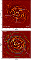 |
Fig. 2 H-band images of AB Aur (October 2023), showing the main structures. Top panel: scattered light features. Bottom panel: millimetric features (yellow: dust ring; white: 12CO spirals S1 and S2 from Tang et al. (2017); green: SO ring and SO peak from Dutrey et al. (2024); blue: C18O ring from Dutrey et al. (2024) and pink: out of plane spirals (or streamers) St1, St2, and St3 from Speedie et al. (2025). The central yellow cross indicates the star’s position. Images are normalized by r2 and spatially filtered. North is up and east is left. |
2.3 Accuracy of the image orientation
The quality of the data and the stability of the instrument allow a detailed dynamical analysis, particularly of the rotation of disk structures. We therefore first assessed the accuracy of the image orientation. Maire et al. (2016) demonstrated that the true north is oriented at −1.75 ± 0.08° with IRDIS in pupil-tracking mode. The pipeline corrects this absolute misalignment. To measure the relative uncertainty between the three epochs, we calculated the position of a background star (detected in total intensity but not in DPI) located at ∆α = −6.326″ and ∆δ = 0.646″, while the proper motion of AB Aur is μα = 4.018 mas/yr and μδ = −24.027 mas/yr. We calculated a difference between the expected and the measured position angle of 0.03° between epochs 1 and 2, and less than 0.01° between epochs 2 and 3, so we adopted 0.03° as the global absolute error on the image orientation. Owing to this accurate calibration of the image orientation, disk rotation becomes an obvious characteristic when visually comparing the three epochs. To illustrate the counterclockwise motion, we overlay the contours of epoch 1 and epoch 3 in Fig. 3 and we provide an animation online.
2.4 Dynamics of the disk
We first analyze the global dynamics of the disk. To this end, we deprojected the images to measure the dynamical evolution in the plane of the disk. To estimate the dispersion of the measurements, we considered variations of the disk PA (55° and 60°) and disk inclination (20°, 25°, and 30°), based on the literature (Di Folco et al. 2009; Tang et al. 2017; Betti et al. 2022). Ren et al. (2020) devised a method to estimate the velocity of spiral arms that involves precisely locating the spiral spine and fitting a spiral model. With the current data, this approach would be impractical because of the complex morphology of AB Aur, including the irregularity of the spirals, possible confusion between all structures, and uncertainty regarding the connection between features. Therefore, we propose an alternative approach in the following, which also has the advantage of measuring the velocity as a function of separation from the star.
Because we expect differential rotation due to the Keplerian motion of the disk material, we divided the deprojected images into several rings. Their corresponding angular radii range from 0.1″ to 0.6″ in steps of 0.1″, and from 0.6″ to 2.4″ in steps of 0.2″, spanning physical distances of 15-370 au in the disk plane. For each annulus, we solved for the optimal rotation and flux ratio between each pair of epochs that minimizes their quadratic difference. Before the minimization, the Qφ images were highpass filtered by subtracting a blurred boxcar image (width 12 pixels; 1 pixel = 12.25 mas), and multiplied by r2, the square of the stellocentric distance (this normalization has little effect because of the ring-wise breakdown). We plotted the angle of rotation for each separation bin and compared this quantity to the expected Keplerian rotation in the disk plane as a function of distance, assuming M* = 2.4 M⊙ (DeWarf et al. 2003). We verified that the scale height of the disk has little impact on this Keplerian profile. We calculated the error bars from the standard deviation of the six realizations of the parameter pairs (PA and inclination), quadratically added to the minimization error derived from the covariance matrix, and we forced the minimal error to be 0.03°, corresponding to the image-orientation accuracy.
Figure 4 presents the angle of rotation between two epochs. This analysis unambiguously demonstrates that the AB Aur disk globally follows counterclockwise rotation in the disk plane (hence the negative values). The amplitude of the rotation reaches about −7° at the smallest achievable separations (about 15-30 au, equivalent to 0.1-0.2″ in the sky plane) and converges to 0° at the largest separations. The measurements agree well with the expected rotation amplitude for Keplerian motion (shown by the blue lines in Fig. 4), particularly beyond a typical distance of ~50 au. However, the agreement is poorer inward, as seen in the residuals, indicating either that the disk rotates more slowly than the local Keplerian velocity or that temporal morphological changes do not allow for a sufficiently accurate measurement of the velocity. We performed the same analysis on each spiral arm separately using a mask to isolate the relevant pixels (results are shown in Fig. B.1). Although we only probed the inner part of the disk (<100 au) where the spirals S1 and S2 are located, we measure the same kind of behavior in the full image, with a deviation at physical distances smaller than 50 au.
This similarity between the whole disk behavior and that of the spirals can be explained by the high-pass filtering of the data, which already selects the spirals as the main structures in the image.
In addition to this ring-wise approach, we also measured the rotation of features as if they were each undergoing a solid-like rotation, using the same minimization methodology between two epochs. Table 2 reports the values, and the error bars correspond to the dispersion of the measurements for the six deprojection parameters. The feature names correspond to the masks shown in Fig. B.1. We find that the spirals S1 and S2 behave differently, with the rotation of S2 progressing more linearly with time (about −2.1° between the closest epochs in time and about −4.5° over the longest temporal baseline), while it is more difficult to identify a clear trend for S1. Again, such measurements can be biased by the morphological evolution of the features, but they can also indicate different dynamical behaviors and possibly different origins for S1 and S2.
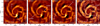 |
Fig. 3 H-band images of AB Aur at three epochs in a 1″ × 1″ field of view. The rightmost panel displays the contours of epoch 1 (dashed line) and epoch 3 (solid line) superimposed on the image from epoch 3. Images are spatially filtered. North is up and east is left. |
Rotation of the main features.
2.5 Dynamics of individual features
The disk of AB Aur is composed of several characteristic features that may have a different dynamical behavior than the disk itself. Measuring their evolution is important to ultimately derive constraints on perturbating bodies. In this section, we specifically analyze the motion of f1, f2, and f3 (located at 0.17″, 0,67″, and 0.19″ from the star, respectively), and the bridge. We proceeded similarly as for the disk: we isolated each feature with a numerical mask and computed the angle of rotation that minimizes the residuals between two epochs. For f1, f2, and f3, we also measured their position in each individual epoch by Gaussian fitting. This required tighter masking to avoid contamination with other extended spiral features of the disk, which inevitably yielded larger dispersions. However, we emphasize that both methods can be biased by the disk environment, even when the dispersion is small. Nevertheless, both methods are consistent, although the error bars are larger for the latter. Fig. 5 reports the measurements.
Visually, all features show a clear unambiguous counterclockwise rotation, except f2, which appears almost static. However, according to the analysis, none of the features perfectly follows the Keplerian rotation of the disk plane at all epochs. Although f1 is compatible with the Keplerian motion for the 2021-2019 epoch pair (blue circle), it significantly deviates for the 2023-2019 pair (red circle). This behavior can be explained by changes in the shape of the feature itself, which appears more structured in 2023, with a more localized intensity peak. As for f3, which appears radially symmetrical to f1, its rotation is marginally compatible with the Keplerian motion for the 2023-2019 pair (red square), but appears static for the 2021-2019 pair (blue square). The latter result is very likely an issue with the isolation of the feature in the 2021 image. The bridge (triangles) exhibits a clear rotation at all epochs, but the speed is slower than the Kelperian motion. Finally, f2 is the most puzzling because it is almost static, while the surrounding disk features actually vary in rotation. The measurements (diamonds) are also consistent with zero or small rotation amplitudes, although they are marginally compatible with Keplerian when using the Gaussian-fitting method because of larger error bars.
We also performed orbital analyses for f1, f2, and f3. As described in Appendix B.2 and moderated by the small orbital coverage, the main outcome is that the features would likely orbit out of the disk plane with inclinations of 75°, 38°, and 34°, or 32°, 77°, and 78°, for f1, f2, and f3, respectively. The two families of solutions arise from the 180° uncertainty in the position angle of the nodes. For each value, the dispersion of the posterior distribution can reach about 15° to 20°, as shown in the corner plots (Fig. B.3).
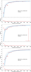 |
Fig. 4 Disk rotation as a function of radius for each pair of epochs. The data points are shown in red, while the blue line represents the expected Keplerian rotation in the disk plane (solid) and for inclinations of 20°, 30°, 40°, and 50° (darkest to lightest lines). The residuals between the data and the Keplerian are shown below each plot. From top to bottom: Epoch 2 vs. epoch 1, epoch 3 vs. epoch 2, and epoch 3 vs. epoch 1. The time interval is given in years. |
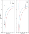 |
Fig. 5 Rotation of the main disk features for two epoch pairs (2021 vs. 2019 in blue and 2023 vs. 2019 in red). The symbols correspond to f1 (circle), f2 (diamond), f3 (square), and the bridge (triangle). Each curve shows the expected Keplerian rotation using the same color coding as the symbols. The left panel shows the results from the optimization method, while the right panel shows results from Gaussian fitting (only for f1, f2, and f3). |
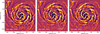 |
Fig. 6 Deprojected H-band images of AB Aur for the three epochs. Dotted lines approximately trace the main shadow patterns identified at each epoch. Images are multiplied by r2 and spatially filtered. The blue, green, and pink circles trace the potential location of clumps that could be casting the shadows. |
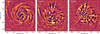 |
Fig. 7 Principal component analysis (PCA) of the three images shown in Fig. 6. Principal components 0, 1, and 2 are shown from left to right. The shadow positions at the first epoch (December 18, 2019) are superimposed. |
2.6 Radial shadows
The disk of AB Aur exhibits several shadow patterns with different morphologies, which presumably correspond to different origins. In Fig. 2, we indicate two distinct broad shadows in the west part of the image, located on either side of the bridge and bounded by spiral arm S1 and the root of S2 (also visible in Fig. 1 prior to filtering). These may be connected to the inner cavity observed in the submillimeter. In this section, we focus instead on the radial, thin shadows that are barely visible in Figs. 1 and A.1. They undergo azimuthal rotations, mostly revealed visually by blinking between epochs (see the online animation), from which we can constrain the distance at which they originate. We label these nearly (but not exactly) radial shadows in Fig. 6. Some are consistent across epochs but show measurable rotation, not necessarily centered on the star, while others show faster variability.
To visually enhance the shadows, we applied a principal component analysis (PCA) to the set of three H-band images to identify static and moving features across the epochs. Qualitatively, we obtained the best visibility using deprojected, r2 normalized, high-pass filtered images, as shown in Fig. 7, which displays the three principal components. While the first mode (PC#0) represents the quasi-static main structures across the three epochs, the two other modes (PC#1 and PC#2) emphasize radial structures. We note that since the principal components are built on the temporal dimension, PC#1 and PC#2 do not directly trace the locations of the radial shadows, but provide an indication of the areas covered by the shadows over time. We describe the observed properties of the shadows in the following.
The four features sh1, sh4, sh5, and sh6 are broadly aligned with the bridge, the feature f3, the pinhole, and f1, respectively.
The feature sh3 shows a clear azimuthal rotation of about 12° between the first and last epochs (3.847 years). Assuming Keplerian motion in the disk plane and a circular orbit, this is consistent with a shadow cast by an object or a local optically thick clump at an orbital distance of about 31 au. Fig. 6 shows the approximate position of such a clump, marked by a blue circle.
Feature sh3 also overlaps with f2, producing a dimming of the feature that is strongest in 2021. Relative to its mean flux measured in spatially filtered images (unfiltered images are disk-dominated), f2 varies by −14, −20, and +33% in 2019, 2021, and 2023. This places a strong constraint on the nature of f2, which therefore cannot be a self-luminous object in the near-IR, and instead is a scattered-light feature.
The shadow sh1, which extends the bridge, varies by 6°, equivalent to 50 au, corresponding exactly to the distance where we detect the outer edge of the bridge (green circle in Fig. 6).
The shadow sh2 has a lower rotation amplitude of about 4°, corresponding to a distance of 66 au (pink circle in Fig. 6).
Feature sh6 is located in the radial direction away from the hot spot mentioned by Tang et al. (2017) and the feature f1 identified by Boccaletti et al. (2020). It is also sweeping in the direction of AB Aur b. Whether it is related to its Hα variability remains to be investigated (Bowler et al. 2025).
While Fig. 6 shows the possible locations of opaque clumps that are consistent with the azimuthal variation of the shadows, there are no associated clumpy features in the image. However, shadows may also be cast by a structure with some vertical extent, such as a spiral arm crossing the midplane. This is the case for sh3 (blue circle connected to the northern arm of the spiral S2) and for sh1 (green circle connected to the bridge). Similar radial shadows have been observed in MWC 758. Based on 3D hydrodynamical simulations, Calcino et al. (2020) conclude that the shadows were cast by optically thick regions of the spiral arms rather than by an inclined inner disk, as in HD 142527 (Marino et al. 2015), consistent with what is observed in AB Aur. Shadows observed in scattered light can also be related to the local vertical extent of the disk, where a feature such as f1, or even the entire spiral arm, traces bumpiness on top of the disk average surface, thereby casting a shadow behind it.
Additionally, using the framework developed by Akansoy et al. (2025), we tentatively estimated the mass of objects that could cast radial shadows. As the results are not fully conclusive, we report this analysis in Appendix C.
2.7 Discussion on dynamics
2.7.1 Keplerian rotation
Our multi-epoch data set allows us to trace rotation patterns for a variety of disk structures. To our knowledge, we detect the global Keplerian rotation of the disk here for the first time through the investigation of scattered-light variations. Our analysis assumes that small-scale structures in the spatially filtered images persist across epochs. Our estimate of the rotation is broadly consistent with a Keplerian pattern around a 2.4 M⊙ central star down to a stellocentric distance of about 60 au (Fig. 4), whereas all three epoch combinations consistently show slower rotation in the inner regions of the disk cavity, down to the edge of the coronagraphic mask (also in Fig. B.1). Tang et al. (2017) report Keplerian patterns for the inner eastern and western CO spirals S1 and S2 using Doppler velocity measurements with ALMA (see their Fig. 3), whereas our IR observations trace motions projected onto the sky plane. Although planet-induced spirals are expected to rotate at the orbital speed of the planetary companion, Keplerian motion is instead expected for spirals induced by gravitational instabilities (Cossins et al. 2009; Yoshida et al. 2025). This may be particularly relevant for the large-scale spirals beyond ~150 au.
Speedie et al. (2024) recently proposed a gravitational instability scenario to account for wiggles occurring in the velocity field of outer CO spirals beyond ~160 au (outside the cavity) and argue that the disk mass may represent a third of the stellar mass. In that case the estimate of the Keplerian velocity would be biased, as the disk mass would be smaller at smaller stellocentric distances, which could effectively slow the rotation of the disk. However, Calcino et al. (2025) dispute this interpretation and find that late infall produces signatures similar to those of gravitational instability. This scenario may apply to the outermost spiral arms of the disk. Moreover, the distance at which the disk rotation starts to depart from a Keplerian motion corresponds to the inner disk cavity, where both gas and millimeter-size grains are depleted. Furthermore, most spiral motions investigated through multi-epoch measurements have so far favored the companion-disk interaction scenario over gravitational instability (e.g., Xie et al. 2023). As a sanity check, we used the approach in Fig. 4 to estimate the stellar mass that can cancel out the residuals at the smallest physical separations of about 50 au. We find values close to 1 M⊙ (or even lower) for the longest temporal baseline, which is unrealistic given the spectral type of the star. Therefore, the measured disk rotation does not seem to support a strong impact from the disk mass.
2.7.2 Deviations from Keplerian rotation
In the central regions of the millimeter cavity, the velocity discrepancy may arise either from a true variation in the angular frequency or from artifacts. If the observed slower rotation has a physical origin, it may be linked to interactions with one or several gravitational perturbers located within the cavity. In the case of a companion on a circular orbit, the entire spiral arm rotates at the perturber’s frequency (e.g., Xie et al. 2024). Because the positive shifts of the residuals of the rotation angles in Fig. 4 have different amplitudes for the three innermost annuli (the largest deviation is usually found for the innermost annulus around 22 au), a single gravitational perturber can hardly account for the observed trends. Within 60 au, our measurement is greatly influenced by the presence of three main bright structures: S1, S2, and the bridge. We therefore investigated the motion of the inner spirals S1 and S2 separately using different numerical masks (Fig. B.1), and we also performed the analysis assuming a single rotation speed for each structure (Table 2). If the S1 spiral were generated by interactions with a perturber located at f1 on a circular orbit, it should rotate much faster than the local Keplerian value, in contrast to our findings. Conversely, if S2 were generated by interactions with a perturber located at AB Aur b, it should rotate slower, at the Keplerian speed corresponding to a ≃ 75 au (according to the preliminary orbital fit proposed in Currie et al. 2022). Only S2 yields a consistent angular velocity across the three epochs, with a mean value of about 1.2deg.yr−1 (Table 2). Therefore, we cannot completely exclude a dynamical link between S2 and the AB Aur b candidate, whereas the motion of S1 appears too slow to be connected with the f1 candidate. We also note that we did not identify a protoplanet candidate in the wake of S2 that could correspond to the Dong et al. (2016) prediction.
The situation is more complex if the perturber’s orbit is eccentric. A planet on an eccentric orbit can generate multiple spiral arms with significant deviations from Keplerian speed and with angular frequencies that depend on the orbital phase (Fig. 11 in Zhu & Zhang 2022). In this respect, the presence of detached or broken spiral arms and bifurcations in AB Aur is also reminiscent of the structures expected from eccentric planets, but the complicated patterns make their identification quite challenging.
Alternatively, deviations from Keplerian speed could also be attributed to the following artifacts: (1) the ability to measure rotation close to the star at very short angular separations; (2) structural or illumination changes with a shorter timescale closer to the star, which would bias our measurement process (although this would hardly explain the systematic positive shift in the measured rotation angles); and (3) deprojection effects. We emphasize that any structure that is not coplanar with the outer disk midplane would appear closer to the star due to simple projection effects and may artificially produce a slower apparent rotation. Indeed, an inclined Keplerian curve provides a slightly better agreement with our measurements (lines with various shades in Figs. 4 and B.1), but it cannot account for the largest deviations at the smallest angular separations. For simplicity, we used a geometrically thin disk approximation in the deprojection step, which does not account for the altitude or flaring of the scattered-light surface; however, the modest disk inclination should mitigate such an artifact. Inclined structures up to 25-45° with respect to the disk midplane have previously been reported and interpreted as infalling material Tang et al. (2012); Speedie et al. (2025), but these are located in the outer disk region.
Moreover, the bright radial feature labeled the bridge has a motion roughly consistent with a solid rotation pattern, with a constant speed of ~1.3 deg.yr−1 across the three annuli (Fig. B.1). It is tentatively associated with a low signal to noise (S/N) feature reported in the HCO+ emission by Rivière-Marichalar et al. (2019) with NOEMA (NOrthern Extended Millimeter Array). It casts a deep and broad shadow onto the S2 spiral (Figs. 2, 3, 6 with the label sh1), which suggests either a larger vertical thickness or a tilted, optically thick component for this filament with respect to the surrounding material.
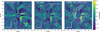 |
Fig. 8 Principal component analysis (PCA) reduction in ADI using ZIMPOL for the two filters CntHα (left) and N_Hα (middle and right). The rectangle indicates the aperture used for photometry. Structures oriented along the diagonal of the images at about 0.35″ from the star are produced by the SPHERE deformable mirror (DM). The right subpanel shows the IRDIS DPI J-band contours overlaid on the ZIMPOL NHα PCA image. The intensity scale is in contrast relative to the star. North is up and east is left. |
3 SPHERE/ZIMPOL Hα imaging
3.1 Observations and data reduction
We obtained observations with ZIMPOL on October 29, 2021 (P108, see Table 1 for the Log) in imaging configuration using the pupil-tracking mode. The dichroic was set to the DIC_HA position to optimize the photon sharing, sending the R band to ZIMPOL and the remaining bandwidth to the wavefront sensor. The coronagraph configuration corresponds to V_CLC_M_WF, which is a suspended 155 mas diameter opaque Lyot mask in the focal plane, combined with a 78% transmission pupil stop. We used the NHα and CntHα filters simultaneously for each ZIMPOL arm, centered in (λ0=656.34 nm) and out (λ0=644.90 nm) of the Hα line, but have different bandwidths (0.75 and 3.83 nm, respectively; Schmid et al. 2017). Science frames with the source on the coronagraph total an integration time of 5760s (392 frames of 15s each). We also obtained out-of-mask PSFs for flux normalization. The parallactic angle varies by a total of 28.6°.
The High Contrast Data Center (Delorme et al. 2017) processed the data using standard cosmetic reduction steps, including dark subtraction, flat-field correction, and bad-pixel removal. We further rejected remaining bad pixels using sigma clipping and subtracted the median of each column to remove detector artifacts, masking the central 200-pixel radius region to avoid biasing the median with the star flux. Fig. D.1 shows images of the target on and off the coronagraph. Next, we processed the data cubes using a PCA-based angular differential imaging (ADI) method following Soummer et al. (2012). Fig. 8 presents the results for two-mode truncation.
The ZIMPOL PCA images reveal astrophysical signals that are coincident with the position of f1, the northern part of spiral S2, and the bridge, as well as diffraction patterns, that are either radial (attributed to the mask support and the deformable mirror correction) or located at the AO correction radius (at 0.28″-0.42″, Fig. 9), which is strongest at PA = 30-60°. Investigating whether real sources exist (in particular the faint source circled in yellow southeast of the star at [δRA, δDec] = [0.30″, −0.17″]) in the region contaminated by the correction radius would require additional observations. These possible artifacts are clearly less dominant in the N_Hα filter image, while the brightest feature coincides with the position of f1. In contrast to the smooth profile observed for f1 in the near-IR, its shape appears elongated north-south, and patchy with three distinct knots, in both CntHα and NHα . Due to the nearly two times smaller bandwidth, the S/N in the NHα filter is worse than in the continuum. We note that f2 and f3 are undetected. We discuss the detection of AB Aur b in Section 3.4, and we also report in Fig. 9 the recent detection of a companion candidate in 12CO ro-vibrational transitions (Kozdon et al. 2026), which again results in a non-detection in Hα with ZIMPOL in a region that is not attenuated by the coronagraph spiders.
To verify the reliability of the features detected in Hα , we overplotted contour lines from the 2021 IRDIS DPI J-band image onto the ZIMPOL NHα image in Fig. 8 (right). While this unambiguously confirms the connection between the visible features and near-IR features at the location of f1, the recovery of the bridge is more questionable. Given that the coronagraph mask in the focal plane is suspended by four spiders in a fixed orientation while the field rotates in pupil-tracking mode, it is important to verify the potential obscuration of real disk features. Figure D.3 shows the area swept by the spiders in the field of view. As a result, the feature f1 is not impacted by the spiders, in contrast to the bridge and, to a lesser extent, AB Aur b. Therefore, in the following, we consider that the bridge signal is altered too much by the coronagraphic mask’s spiders to extract reliable photometry. We note that despite the attenuation due to these spiders, some regions of the disk have no Hα counterpart, like for instance the east-northern part of S1. Although located at a similar physical distance to f1, the regions should have a brightness ratio similar to that measured in the near-IR if it were dominated by scattered light. This observational fact possibly argues in favor of a distinct Hα emission at f1.
Attempts to combine angular and spectral differential imaging by subtracting the images in the two filters were not satisfactory and are therefore not shown. We suspect that the difference in the filter bandwidths prevents such a process. We describe the procedure used to estimate the Hα flux emission in the next section.
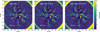 |
Fig. 9 Images in NHα (left), with a fake planet (FP) injected at the flux of AB Aur b (middle) and with twice the flux (right). Labels indicate the position of the candidate planet. The dashed circles trace the region contaminated by the AO correction radius, while the pink cross represents the companion candidate reported in Kozdon et al. (2026) in 12CO ro-vibrational transitions. The yellow circle at ρ = 0.35″, PA = 119.7° marks a new signal that remains to be investigated. |
3.2 Hα flux and accretion rate
We estimated the flux in the Hα line following Schmid et al. (2017) and Cugno et al. (2019). The method converts the count rates measured in the data into flux in physical units using the tabulated zero points for ZIMPOL in the CntHα and NHα filters. We then estimated the continuum contribution in the NHα filter to isolate the Hα flux alone. Appendix E.2 details the calculations of FHα. Next, we derived the luminosity directly from the Hα line flux
 (1)
(1)
To estimate the accretion luminosity (Lacc), we considered two approaches. The first approach is based on empirical calibrations of the relationship between LHα and Lacc. Most studies have so far used the calibration for classical T Tauri stars (CTTS; Rigliaco et al. 2012), which involves strong magnetic fields and was updated by Alcalá et al. (2017, Al2017). More recently Aoyama et al. (2021a, Ao2021) provided an updated model for shock emission at the planetary surface that is more relevant for protoplanets. The second approach is based on 3D thermohydrodynamical simulations of planet formation (Szulágyi & Ercolano 2020, SE2020). The former case implies magnetospheric accretion which operates when the magnetic field exceeds approximately 60 G, whereas the latter involves boundary-layer accretion occurring for weaker magnetic fields. We provide the corresponding relationships, Lacc versus LHα, for the different models in Appendix E.2.
In the CTTS and shocks framework, the accretion rate follows
 (2)
(2)
where R and M are the radius and the mass of the accreting object, Rin is the truncation radius of the circumplanetary disk, and G is the gravitational constant. Most terms in this equation are undefined, so we adopted standard assumptions: R = 1 RJup, M = 1 MJup, and Rin = 5 R. We then derived a tentative estimate of the object mass at the system age under the assumption of a constant accretion rate. This assumption neglects accretion variability.
In contrast, the model of Szulágyi & Ercolano (2020) provides a direct relationship between the line luminosity and the planet mass,
 (3)
(3)
3.3 Photometric measurements
3.3.1 Stellar accretion
We first estimated the stellar accretion rate. We integrated the signal within an aperture radius of 1.5″ to encompass the full PSF. We measured FCntHα = 7.10 × 10⁻¹¹ erg/s/cm2 and FNHα = 5.78 × 10⁻¹¹ erg/s/cm2, which yield a line-to-continuum ratio of 241% and therefore a flux for FHα = 4.09 × 10⁻¹¹ erg/s/cm2. We used the relation from Mendigutía et al. (2011) (similar to Eq. (E.5a) but with different coefficients) calibrated for the Hα line in HAeBe stars instead of Alcalá et al. (2017) which holds for CTTS. The corresponding mean accretion luminosity is Lacc = 4.32 L⊙, with a mass accretion rate of Ṁacc = 1.80 × 10⁻⁷ M⊙/yr, which is consistent, despite the large dispersion, with other estimates based on Brγ (Lacc = 4.26 L⊙; Garcia Lopez et al. 2006) and Pfβ (Lacc = 3.16 L⊙; Salyk et al. 2013).
3.3.2 Photometry and accretion at f1
We now focus on f1, the main feature in the NHα filter. However, applying accretion models to extended features is questionable, as protoplanets or a circumplanetary disk should exhibit a more compact morphology. However, f1 appears to be substructured with knots, although their reliability remains to be confirmed with further observations. We therefore considered the brightest knot identified in Fig. 8, located in the middle of f1. We first estimated the attenuation of the PCA processing on f1, given that the true morphology and intensity distribution of the structure are unknown. For this purpose, we used forward modeling and for simplicity we assumed a fake feature with a Gaussian shape, the size of which (2 × 2 pixels) is representative of the knot. We projected this model onto the same eigenbasis and with the same mode truncation as that used for the data. This modeling allowed us to estimate an attenuation of a factor of 2.37 (assumed to be constant for both filters) in the photometric aperture due to PCA, which we used to compensate for the count rate loss. In addition, we accounted for coronographic transmission. For this, we built a data cube with a binary mask representing the central spot and the spiders of the coronagraphic mask, rotated according to the parallactic angle variation. Summing these frames and normalizing yields an estimate of the transmission projected on the sky. In the photometric aperture defined for the knot f1, we measured a transmission of unity. We then estimated the flux in each filter: FCntHα = 4.38 × 10⁻¹⁵ erg/s/cm2 and FNHα = 2.63 × 10⁻¹⁵ erg/s/cm2, which yields a line-to-continuum ratio of 151% and therefore a flux of FHα = 1.58 × 10⁻¹⁵ erg/s/cm2.
Using the relation from Alcalá et al. (2017) and assuming a truncation radius of five times the radius of the accreting object, we find Lacc = 3.65 × 10⁻⁶−3.42 × 10⁻⁵ L⊙ and Ṁacc = 8.02 × 10⁻⁸−7.52 × 10⁻⁷ MJup /yr. The ranges of these values correspond to the dispersions of the empirically calibrated relationships of the luminosities described in Appendix E.3. Therefore, the time to accrete 1MJup is 1.4-13 Myrs, assuming a constant accretion rate. Assuming the emission originates from the shocks at the planetary surface (Aoyama et al. 2021a), the accretion luminosity is much higher, with Lacc = 4.84 × 10⁻⁵−1.93 × 10⁻⁴ L⊙, and the corresponding mass accretion rate is Ṁacc = 1.06 × 10⁻⁶−4.23 × 10⁻⁶ MJup/yr. Over 1 Myr, the accretion rate would correspond to 1-4 MJup, significantly higher than in the CTTS framework.
Although extended, f1 appears as a series of knots in Hα, which could correspond to multiple objects. We therefore estimated the total luminosity and accretion rate of the whole structure assuming it was composed of several point sources. We defined an aperture of 10 × 34 pixels optimized to encompass f1 in both the NHα and CntHα filters. Assuming a forward model of an elliptical Gaussian profile with the same extension and position as f1, we derive an attenuation of the PCA processing of 3.75. As previously, we also estimated the attenuation from the coronagraph, which is 0.978. The measured fluxes are FCntHα = 2.00 × 10⁻¹⁴ erg/s/cm2 and FNHα = 1.30 × 10⁻¹⁴ erg/s/cm2 , which yields a line-to-continuum ratio of 172% and therefore a flux of FHα = 8.22 × 10⁻¹⁵ erg/s/cm2. Using the relation from Alcalá et al. (2017), we obtain Lacc = 2.55 × 10⁻⁵−2.03 × 10⁻⁴ L⊙ and Ṁacc = 5.09 × 10⁻⁶−2.02 × 10⁻⁵ MJup/yr. Therefore, the time to accrete 1 MJup is less than 1 Myr, which implies that, for the age of the system, the Hα emission from the whole f1 feature still corresponds to typical masses of giant planets. Using the model of (Aoyama et al. 2021a), the accretion luminosity reaches Lacc = 2.31 × 10⁻⁴−9.22 × 10⁻⁴ L⊙ and thus the mass accretion rate is Ṁacc = 5.08 × 10⁻⁶−2.02 × 10⁻⁵ MJup/yr. Over 1 Myr, this accretion rate would correspond to 5-20 MJup, potentially consistent with several planetary-mass objects. Although we cannot exclude the possibility that the detected emission originates from stellar Hα emission scattered off clumps located along the twisted spiral S1.
3.4 Testing the detection of AB Aur b
The protoplanet candidate AB Aur b has been detected in Hα filters (Currie et al. 2022; Zhou et al. 2022) and at UV wavelengths (Zhou et al. 2023), contrasting with the ZIMPOL data, which show a faint signal at the expected location (Fig. 9). To assess whether this signal could be related to AB Aur b, we used fake planet injection, starting from the flux measured with HST/WFPC3, 1.03 × 10⁻¹⁵ erg/s/cm2/Å, or 7.725 × 10⁻¹⁵ erg/s/cm2, which we converted to count rate by inverting Eq. (E.1b). However, we note that the WFPC3 Hα filter is more than twice as broad as the NHα filter, so using this flux for injecting a fake planet would be valid only if the Hα line dominates over other sources. To account for the spatial extent of AB Aur b we generated the fake planet as a 90 × 60 mas 2D-Gaussian shape, scaling the flux to the exposure of one frame, shifting at 0.6″ south, and rotating with the parallactic angles to account for the field rotation. We reprocessed this new data cube with PCA ADI. Fig. 9 shows the results for the expected planet’s flux and a flux twice as large, both compared to the original image. Therefore, the faint signal observed at the position of AB Aur b is marginally consistent with a detection.
Assuming that the detected signal corresponds to AB Aur b in the NHα filter, we measured the counts and applied the same calculation as for f1. We defined an elliptical aperture of 90 × 60 mas to match the extension of AB Aur b. The PCA-induced attenuation factor is 1.44, as measured from the fake planet injection step, while the coronagraphic transmission is 0.84. We measure FCntHα = 8.82 × 10⁻¹⁶ erg/s/cm2 and FNHα = 8.57 × 10⁻¹⁶ erg/s/cm2, hence FHα = 6.47 × 10⁻¹⁶ erg/s/cm2, which is approximately 13 times lower than the integrated Hα emission of f1. In the magnetospheric accretion model, this flux corresponds to Lacc = 1.21 × 10⁻⁶−1.30 × 10⁻⁵ L⊙ and Ṁacc = 2.79 × 10⁻⁸−2.86 × 10⁻⁷ MJup/yr. The time required to accrete 1 MJup is longer than 3.7 Myrs and potentially exceeds the system age. Therefore, it is unlikely that the Hα emission corresponds to a planetary-mass object given the age of the system. However, the results differ under the shock model of Aoyama et al. (2021a), which yields an equivalent mass of 0.45-1.81 MJup.
3.5 Discussion on accretion
Accretion rate and mass estimations. Table E.1 compiles all flux measurements for the various features. Overall, the integrated Hα fluxes for f1 and the knot in f1 are consistent with accretion rates expected for objects in the planetary mass regime, but can vary significantly (by up to two orders of magnitude) depending on the model used to convert the Hα luminosity into mass. Table E.1 also lists the luminosity and mass derived using the boundary layer model (Szulágyi & Ercolano 2020). We find significantly larger accretion luminosities with the boundary layer model. However, the estimated masses remain in the same range, typically 6-10 MJ, regardless of the Hα flux.
Huélamo et al. (2022) report similar dispersions of Lacc for other targets. To illustrate the differences, we compare the accretion luminosity as a function of the Hα luminosity for different models in Fig. E.2. The magnetospheric accretion model exhibits a steep dependence; whereas the boundary layer model represents the opposite extreme, with a weak dependence of accretion on Hα luminosity. All models provide consistent results for Hα luminosities larger than about 2 × 10⁻⁵ L⊙, but the features of interest are fainter, leading to a strong dispersion in the accretion rates. However, the models of Szulágyi & Ercolano (2020) and Aoyama et al. (2021a) yield consistent mass estimates for f1, although they originate from different physical conditions. Therefore, the models are difficult to disentangle using Hα luminosity measurements alone. Aoyama et al. (2021b) studied the strengths of hydrogen lines in the visible and near IR as accretion tracers and highlight additional lines such as Paβ (1.282 μm), Brγ (2.166 μm), and Brα (4.052 μm), which help break degeneracies and better constrain the accretion mechanism. However, AB Aur b has not been detected in Paß (Biddle et al. 2024), suggesting that extending observations further into the IR could be useful to take advantage of lower opacities in the main disk.
Detection and non-detection of the features. Interestingly, the very high angular resolution capacity of ZIMPOL allows us to resolve the extended structure f1 as a series of knots, consistently in both filters. Whether this morphology is affected by the data reduction process, which subtracts the starlight and may introduce self-subtraction, or by partial obscuration from the coronagraphic mask spiders, remains to be determined. These observations require confirmation and/or finer observations. At present, ZIMPOL is the only instrument capable of such observations with this level of contrast and proximity to the star. We note that f1 has not been reported in SCExAO observations (Currie et al. 2022) or with HST/WFPC3 (Zhou et al. 2022), as it lies beyond the reach of these instruments. Conversely, the non-detection of f2, which is farther from the star than f1, supports the hypothesis of a scattered-light feature, since the scattered light decreases with the square of the physical distance to the star. Nevertheless, this is not the case for f3, which lies at the same separation as f1, so its non-detection requires another explanation. High-contrast imaging instruments operating at visible wavelengths on the Extremely Large Telescope will be transformative in this regard.
Non-detection of AB Aur b. The very low level of detection of AB Aur b with ZIMPOL is at odds with previous observations obtained in Hα filters, even after accounting for the coronagraph transmission (Currie et al. 2022; Zhou et al. 2022), which report detections at levels about an order of magnitude stronger than ours. However, comparison with other data sets can be complicated by the variable nature of the source, as measured by Bowler et al. (2025), who report a variability amplitude of 330% using HST/WFPC3. Another effect that can attenuate the observed flux of AB Aur b is related to the line profile itself. Using VLT/MUSE, Currie et al. (2025) recently identified an inverse P Cygni profile centered on the Hα line at 6562 À, with a positive flux in the blue wing and a stronger negative flux in the red wing, which could result in a very faint or even negative flux if integrated in a narrow-band filter. However, observations with SCExAO/VAMPIRES, HST/STIS, and HST/WPC3 detect the object. To reconcile these spectroscopic and photometric observations, Currie et al. (2025) argue that the Hα emission may arise from a combination of several sources including scattered light from the disk, and Balmer continuum plus line emission. In this respect, we note that the main difference is that the ZIMPOL filter is narrower (7.5 À) than those of other instruments: VAMPIRES (10 À), WFPC3 (17.9 À), while STIS is unfiltered, and the MUSE line width is about 5 À. Therefore, ZIMPOL images could be more affected by the P Cygni profile, yielding a nearly zero flux. It would be relevant to test this hypothesis with other accretion lines in future observations, in particular Brα and Brγ tracers in the IR, which may be less affected by disk opacity.
3.6 Constraints on binarity
The first hint of a possible companion star around AB Aur was reported by Baines et al. (2006) based on spectroscopic constraints (positional shifts across the Hα line and variations in the FWHM). However, the authors could only infer a binary separation in the range 0.5-3.0″, with uncertain constraints on the position angle. Poblete et al. (2020) produced hydrodynamical simulations of a disk perturbed by a binary star to account for the spiral arms detected with ALMA inside the dust-continuum cavity. They find that a binary star on an eccentric orbit (e=0.5), perpendicular to the disk midplane, with a semi-major axis of 40 au (0.25″) and a mass ratio of 0.25, can qualitatively reproduce the spiral arms observed in CO. With a mass of 0.6 M⊙, this hypothetical companion corresponds to a K4-5 star and would have flux ratios relative to the primary of ΔH = 3.25 and ΔKs = 3.07. Such a component would be very bright unless it is hidden by some obscuring material due to a combination of disk midplane opacity and orbital configuration, or if it lies behind SPHERE’s coronagraphic mask (0.2″ diameter, equivalent to 33 au). Given that SPHERE achieves a contrast better than 10 mag at this angular separation (Boccaletti et al. 2020), the extinction must be larger than 7 mag for such a binary component to remain undetected. Although no such object has been detected during several years of observations of AB Aur, we cannot completely exclude a binary system, even if it appears rather unlikely.
To investigate closer-in perturbers, we used the Gaia PMEX tool (standing for Gaia DR3 proper motion anomaly and astrometric noise excess) developed by Kiefer et al. (2025), which computes the Gaia astrometric excess (based on the renormalized unit weight error and the astrometric excess noise) and accounts for the Gaia-Hipparcos proper motion anomaly. Under the assumption that the excesses are due to a companion, GaiaPMEX provides solutions in a mass-semi-major axis diagram. Lagrange et al. (2025) and Lagrange et al. (in rev.) present examples of its use for the detection of companions. By constraining the inclination to 49-51° (to match the analysis in Section 2.5) and the eccentricity to 0.0-0.3, the astrometric constraints would favor a brown dwarf or stellar component closer than ~1-2 au and more massive than ~50-100 MJupiter (Fig. 10), with a degeneracy toward higher masses at smaller separations. However, we note that a massive companion on such a close orbit would gravitationally disturb, or even disrupt, any inner CSD, which appears inconsistent with the IR interferometric detections of a warm dust disk or ring in the 0.5-10 au inner region of AB Aur (Eisner et al. 2004; Tannirkulam et al. 2008; Di Folco et al. 2009; Lazareff et al. 2017). This analysis does not exclude the solution proposed by Poblete et al. (2020) because Gaia and Hipparcos do not have the sensitivity to detect an astrometric signature for a companion orbiting at 40 au. Blakely et al. (2026, submitted to AJ) obtained comparable results in terms of mass and separation solutions. However, it is important to note that accretion onto the star adds degeneracy in the interpretation of the residuals as discussed in Lagrange et al. (2025, submitted to A&A). The amplitude of this effect depends on both the accretion luminosity and the geometry of the accretion region. In such cases, we argue that attributing the astrometric excess solely to the presence of a companion requires caution, until detailed modeling of the accretion feature is available.
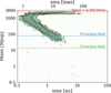 |
Fig. 10 GaiaPMEX analysis for AB Aur showing the solutions (green shades) at 1, 2 and 3 σ in a mass/semi-major axis (sma) diagram. |
4 Conclusions
In this paper we present new observations of the AB Aur system in near-IR bands with SPHERE/IRDIS at three epochs spanning about 3.85 years, and with SPHERE/ZIMPOL in Hα filters, with the aim of studying the dynamics of the disk and the accretion regions. In the following, we summarize our findings.
The disk morphology observed over three epochs shows strong consistency, both in large-scale structures and small-scale structures. This high level of stability is an important asset for dual polarimetry observations with SPHERE/IRDIS, enabling detailed and robust dynamical analyses.
We recovered all features reported in Boccaletti et al. (2020), and we identify new ones, namely the inner spiral arms S1 and S2, the pinhole in S1, the bridge, and the localized features f1, f2, and f3. The three localized features are compact structures or point-like sources. The feature f1, initially identified as a near-IR twist, is resolved as an assembly of knots at shorter wavelengths. Therefore, their morphology contrasts with the broad spatial extent of AB Aur b, possibly indicating a fundamentally different nature.
Differential rotation of the disk is an obvious feature when comparing the three epochs. We developed a method to measure the rotation rate as a function of the radius and find that the disk globally follows a Keplerian rotation, except in the inner regions within ~60 au where the velocity is slower. We observe the same behavior in parts of the brightest spiral arms within the millimeter cavity.
Motivated by the very small motion of f2, we used orbitize! to constrain the orbital solutions for f1, f2, and f3, despite the limited orbital coverage and the spatial extent of f1. We obtain posterior distributions for the orbital inclinations, which favor orbital motions outside the disk plane. For each feature, we find two possible inclinations from the disk midplane: 75° and 32° for f1 , 38° and 77 for ° f2, and 34° and 78° for f3. We note that the dispersion on these values can range from 15° to 20°.
Several radial shadows are visible in the images and we can roughly follow their rotation across the epochs. These shadows are very narrow, likely indicating the presence of optically thick regions at stellocentric distances of 30 to 70 au.
The departure from Keplerian motion within ~60 au could be related to difficulties in precisely measuring the innermost separations as the disk morphology is intrinsically variable. However, in that case, the departure should be random, whereas it is systematically negative in our data. Out-ofplane structures, and more generally the vertical structure of the disk, could also bias the measurements toward slower velocities. Nevertheless, a reasonable interpretation is that the inner 60 au of the disk is gravitationally perturbed by several bodies, consistent with the dynamical behavior of the shadows and with the complexity of the spiral structures.
While the velocity of a spiral arm has been considered as a way to constrain its origin (self-gravity versus gravitational perturbers), in real systems the multiplicity, as well as noncircular and noncoplanar orbits of hypothetical perturbers, complicate this simplistic framework. In this context, we note that given their velocities, the spiral S1 may have been triggered by gravitational instability rather than being launched by f1, although this conclusion relies on the simplified case of a single perturber on circular orbit. However, a dynamical link between the spiral S2 and AB Aur b cannot be ruled out at this stage.
The excess noise in Gaia astrometric measurements, together with the Hipparcos-Gaia proper motion, could suggest a potential binarity of AB Aur. However, we cannot draw firm conclusion since stellar accretion is neglected in astrometric analyses and can also affect the astrometric signal.
Hα imaging with SPHERE/ZIMPOL reveals a strong feature matching f1 in the near-IR. This is the first time this structure is observed in the visible, highlighting the performance of SPHERE. For the Hα line emission, we measure 8.22 × 10⁻¹⁵ erg/s/cm2 for the f1 6.23 × 10⁻⁶ erg/s/cm2 for f1. In contrast, AB Aur b is likely at the limit of detection, with a flux of 6.46 × 10⁻¹⁶ erg/s/cm2
If f1 were a point-source, its flux would correspond to the Hα emission expected for planetary-mass objects, although the conversion to accretion rates or masses is strongly modeldependent.
This study argues in favor of obtaining further follow-up observations to (1) analyze the dynamics of the spiral arms and better understand the implication of the presence of protoplanets, and (2) derive accretion rates from other hydrogen lines at longer wavelengths, in order to break degeneracies in the accretion mechanism and clarify the nature of AB Aur b.
Data availability
A movie is available at https://www.aanda.org
Acknowledgements
This work has made use of the High Contrast Data Centre, jointly operated by OSUG/IPAG (Grenoble), PYTHEAS/LAM/CeSAM (Marseille), OCA/Lagrange (Nice), Observatoire de Paris/LIRA (Paris), and Observatoire de Lyon/CRAL, and supported by a grant from Labex OSUG@2020 (Investissements d’avenir – ANR10 LABX56). This work was supported by the “Programme National de Planétologie” (PNP) and the “Programme National de Physique Stellaire” (PNPS) of CNRS/INSU co-funded by CEA and CNES. NH is funded by the Spanish grant MCIN/AEI/10.13039/501100011033 PID2023-150468NB-I00 J.V., is funded from the Hungarian NKFIH OTKA project no. K-147380. This work was also supported by the NKFIH NKKP grant ADVANCED 149943. Project no.149943 has been implemented with the support provided by the Ministry of Culture and Innovation of Hungary from the National Research, Development and Innovation Fund, financed under the NKKP ADVANCED funding scheme.
References
- Akansoy, D., Petrou, H., Ballabio, G., & Penzlin, A. 2025, MNRAS, 540, 3186 [Google Scholar]
- Alcalá, J. M., Manara, C. F., Natta, A., et al. 2017, A&A, 600, A20 [NASA ADS] [CrossRef] [EDP Sciences] [Google Scholar]
- Aoyama, Y., Marleau, G.-D., Ikoma, M., & Mordasini, C. 2021a, ApJ, 917, L30 [CrossRef] [Google Scholar]
- Aoyama, Y., Marleau, G.-D., Mordasini, C., & Ikoma, M. 2021b, arXiv e-prints [arXiv:2011.06608] [Google Scholar]
- Bacon, R., Accardo, M., Adjali, L., et al. 2010, Proc. SPIE, 7735, 773508 [Google Scholar]
- Baines, D., Oudmaijer, R. D., Porter, J. M., & Pozzo, M. 2006, MNRAS, 367, 737 [NASA ADS] [CrossRef] [Google Scholar]
- Betti, S. K., Follette, K., Jorquera, S., et al. 2022, AJ, 163, 145 [NASA ADS] [CrossRef] [Google Scholar]
- Biddle, L. I., Bowler, B. P., Zhou, Y., Franson, K., & Zhang, Z. 2024, AJ, 167, 172 [NASA ADS] [CrossRef] [Google Scholar]
- Blakely, D., Thompson, W., Johnstone, D., et al. 2026, arXiv e-prints [arXiv:2602.07731] [Google Scholar]
- Blunt, S., Nielsen, E. L., De Rosa, R. J., et al. 2017, AJ, 153, 229 [Google Scholar]
- Blunt, S., Wang, J. J., Angelo, I., et al. 2020, AJ, 159, 89 [NASA ADS] [CrossRef] [Google Scholar]
- Boccaletti, A., Folco, E. D., Pantin, E., et al. 2020, A&A, 637, L5 [NASA ADS] [CrossRef] [EDP Sciences] [Google Scholar]
- Boer, J. d., Langlois, M., Holstein, R. G. v., et al. 2020, A&A, 633, A63 [NASA ADS] [CrossRef] [EDP Sciences] [Google Scholar]
- Bowler, B. P., Zhou, Y., Biddle, L. I., et al. 2025, AJ, 169, 258 [Google Scholar]
- Calcino, J., Christiaens, V., Price, D. J., et al. 2020, MNRAS, 498, 639 [CrossRef] [Google Scholar]
- Calcino, J., Price, D. J., & Ormel, C. W. 2025, arXiv e-prints [arXiv:2510.05601] [Google Scholar]
- Close, L. M., Van Capelleveen, R. F., Weible, G., et al. 2025, ApJ, 990, L9 [Google Scholar]
- Cossins, P., Lodato, G., & Clarke, C. J. 2009, MNRAS, 393, 1157 [Google Scholar]
- Cugno, G., Quanz, S. P., Hunziker, S., et al. 2019, A&A, 622, A156 [NASA ADS] [CrossRef] [EDP Sciences] [Google Scholar]
- Currie, T., Lawson, K., Schneider, G., et al. 2022, Nat. Astron., 6, 751 [NASA ADS] [CrossRef] [Google Scholar]
- Currie, T., Hashimoto, J., Aoyama, Y., et al. 2025, ApJ, 990, L42 [Google Scholar]
- Delorme, P., Meunier, N., Albert, D., et al. 2017, SF2A-2017: Proceedings of the Annual meeting of the French Society of Astronomy and Astrophysics, eds. C. Reylé, P. Di Matteo, F. Herpin, et al., 347 [Google Scholar]
- DeWarf, L. E., Sepinsky, J. F., Guinan, E. F., Ribas, I., & Nadalin, I. 2003, ApJ, 590, 357 [NASA ADS] [CrossRef] [Google Scholar]
- Di Folco, E., Dutrey, A., Chesneau, O., et al. 2009, A&A, 500, 1065 [NASA ADS] [CrossRef] [EDP Sciences] [Google Scholar]
- Dong, R., Fung, J., & Chiang, E. 2016, ApJ, 826, 75 [Google Scholar]
- Dutrey, A., Chapillon, E., Guilloteau, S., et al. 2024, A&A, 689, L7 [NASA ADS] [CrossRef] [EDP Sciences] [Google Scholar]
- Dykes, E., Currie, T., Lawson, K., et al. 2024, ApJ, 977, 172 [Google Scholar]
- Eisner, J. A., Lane, B. F., Hillenbrand, L. A., Akeson, R. L., & Sargent, A. I. 2004, ApJ, 613, 1049 [Google Scholar]
- Eriksson, S. C., Asensio Torres, R., Janson, M., et al. 2020, A&A, 638, L6 [NASA ADS] [CrossRef] [EDP Sciences] [Google Scholar]
- Fuente, A., Baruteau, C., Neri, R., et al. 2017, ApJ, 846, L3 [NASA ADS] [CrossRef] [Google Scholar]
- Fukagawa, M., Hayashi, M., Tamura, M., et al. 2004, ApJ, 605, L53 [NASA ADS] [CrossRef] [Google Scholar]
- Garcia Lopez, R., Natta, A., Testi, L., & Habart, E. 2006, A&A, 459, 837 [NASA ADS] [CrossRef] [EDP Sciences] [Google Scholar]
- Gratton, R., Ligi, R., Sissa, E., et al. 2019, A&A, 623, A140 [NASA ADS] [CrossRef] [EDP Sciences] [Google Scholar]
- Groff, T. D., Rizzo, M., Currie, T., et al. 2017, in Techniques and Instrumentation for Detection of Exoplanets VIII, ed. S. Shaklan (San Diego, United States: SPIE), 39 [Google Scholar]
- Guerri, G., Daban, J.-B., Robbe-Dubois, S., et al. 2011, Exp. Astron., 30, 59 [Google Scholar]
- Haffert, S. Y., Bohn, A. J., Boer, J. D., et al. 2019, Nat. Astron., 3, 749 [CrossRef] [Google Scholar]
- Hashimoto, J., Tamura, M., Muto, T., et al. 2011, ApJ, 729, L17 [Google Scholar]
- Holstein, R. G. v., Girard, J. H., Boer, J. d., et al. 2020, A&A, 633, A64 [NASA ADS] [CrossRef] [EDP Sciences] [Google Scholar]
- Huélamo, N., Chauvin, G., Mendigutía, I., et al. 2022, A&A, 668, A138 [NASA ADS] [CrossRef] [EDP Sciences] [Google Scholar]
- Jorquera, S., Bonnefoy, M., Betti, S., et al. 2022, ApJ, 926, 71 [Google Scholar]
- Kiefer, F., Lagrange, A.-M., Rubini, P., & Philipot, F. 2025, A&A, 702, A76 [NASA ADS] [CrossRef] [EDP Sciences] [Google Scholar]
- Kozdon, J., Fung, J., Brittain, S. D., et al. 2026, AJ, 171, 250 [Google Scholar]
- Lagrange, A.-M., Kiefer, F., Rubini, P., et al. 2025, A&A, submitted [arXiv:2501.10488] [Google Scholar]
- Lazareff, B., Berger, J.-P., Kluska, J., et al. 2017, A&A, 599, A85 [NASA ADS] [CrossRef] [EDP Sciences] [Google Scholar]
- Maire, A.-L., Langlois, M., Dohlen, K., et al. 2016, SPIE Conf. Ser., 9908, 990834 [Google Scholar]
- Males, J. R., Close, L. M., Haffert, S. Y., et al. 2024, in Adaptive Optics Systems IX, eds. D. Schmidt, E. Vernet, & K. J. Jackson (Yokohama, Japan: SPIE), 8 [Google Scholar]
- Marino, S., Perez, S., & Casassus, S. 2015, ApJ, 798, L44 [Google Scholar]
- Marleau, G.-D., Aoyama, Y., Kuiper, R., et al. 2022, A&A, 657, A38 [NASA ADS] [CrossRef] [EDP Sciences] [Google Scholar]
- Mendigutía, I., Calvet, N., Montesinos, B., et al. 2011, A&A, 535, A99 [NASA ADS] [CrossRef] [EDP Sciences] [Google Scholar]
- Müller, A., Keppler, M., Henning, T., et al. 2018, A&A, 617, L2 [Google Scholar]
- Norris, B., Schworer, G., Tuthill, P., et al. 2015, MNRAS, 447, 2894 [NASA ADS] [CrossRef] [Google Scholar]
- Poblete, P. P., Calcino, J., Cuello, N., et al. 2020, MNRAS, 496, 2362 [NASA ADS] [CrossRef] [Google Scholar]
- Ren, B., Dong, R., Holstein, R. G. v., et al. 2020, ApJ, 898, L38 [NASA ADS] [CrossRef] [Google Scholar]
- Rigliaco, E., Natta, A., Testi, L., et al. 2012, A&A, 548, A56 [NASA ADS] [CrossRef] [EDP Sciences] [Google Scholar]
- Rivière-Marichalar, P., Fuente, A., Baruteau, C., et al. 2019, ApJ, 879, L14 [CrossRef] [Google Scholar]
- Sallum, S., Follette, K. B., Eisner, J. A., et al. 2015, Nature, 527, 342 [Google Scholar]
- Salyk, C., Herczeg, G. J., Brown, J. M., et al. 2013, ApJ, 769, 21 [CrossRef] [Google Scholar]
- Schmid, H. M., Joos, F., & Tschan, D. 2006, A&A, 452, 657 [NASA ADS] [CrossRef] [EDP Sciences] [Google Scholar]
- Schmid, H. M., Bazzon, A., Milli, J., et al. 2017, A&A, 602, A53 [NASA ADS] [CrossRef] [EDP Sciences] [Google Scholar]
- Schmid, H. M., Bazzon, A., Roelfsema, R., et al. 2018, A&A, 619, A9 [NASA ADS] [CrossRef] [EDP Sciences] [Google Scholar]
- Soummer, R. 2005, ApJ, 618, L161 [Google Scholar]
- Soummer, R., Pueyo, L., & Larkin, J. 2012, ApJ, 755, L28 [Google Scholar]
- Speedie, J., Dong, R., Hall, C., et al. 2024, Nature, 633, 58 [NASA ADS] [CrossRef] [Google Scholar]
- Speedie, J., Dong, R., Teague, R., et al. 2025, ApJ, 981, L30 [Google Scholar]
- Szulágyi, J., & Ercolano, B. 2020, ApJ, 902, 126 [CrossRef] [Google Scholar]
- Szulágyi, J., Binkert, F., & Surville, C. 2022, ApJ, 924, 1 [CrossRef] [Google Scholar]
- Tang, Y.-W., Guilloteau, S., Piétu, V., et al. 2012, A&A, 547, A84 [NASA ADS] [CrossRef] [EDP Sciences] [Google Scholar]
- Tang, Y.-W., Guilloteau, S., Dutrey, A., et al. 2017, ApJ, 840, 0 [Google Scholar]
- Tannirkulam, A., Monnier, J. D., Harries, T. J., et al. 2008, ApJ, 689, 513 [NASA ADS] [CrossRef] [Google Scholar]
- Van Capelleveen, R. F., Ginski, C., Kenworthy, M. A., et al. 2025, ApJ, 990, L8 [Google Scholar]
- Wagner, K., Stone, J. M., Spalding, E., et al. 2019, ApJ, 882, 0 [Google Scholar]
- Xie, C., Haffert, S. Y., de Boer, J., et al. 2020, A&A, 644, A149 [EDP Sciences] [Google Scholar]
- Xie, C., Ren, B. B., Dong, R., et al. 2023, A&A, 675, L1 [NASA ADS] [CrossRef] [EDP Sciences] [Google Scholar]
- Xie, C., Xie, C., Ren, B. B., et al. 2024, Universe, 10, 465 [Google Scholar]
- Yoshida, T. C., Nomura, H., Doi, K., et al. 2025, Nat. Astron., 9, 1672 [Google Scholar]
- Zhou, Y., Sanghi, A., Bowler, B. P., et al. 2022, ApJ, 934, L13 [NASA ADS] [CrossRef] [Google Scholar]
- Zhou, Y., Bowler, B. P., Yang, H., et al. 2023, AJ, 166, 220 [NASA ADS] [CrossRef] [Google Scholar]
- Zhu, Z., & Zhang, R. M. 2022, MNRAS, 510, 3986 [NASA ADS] [CrossRef] [Google Scholar]
- Zurlo, A., Cugno, G., Montesinos, M., et al. 2020, A&A, 633, A119 [NASA ADS] [CrossRef] [EDP Sciences] [Google Scholar]
Appendix A IRDIS DPI images
Figure A.1 presents the images of AB Aur in three near-IR broad band filters, and Fig. A.2 the Uφ signal in the H band for the three epochs.
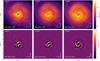 |
Fig. A.1 Same as Fig. 1 but at one period of observations (Nov. 2021 through Jan. 2022) and for the J, H and Ks bands. For visualisation purpose the contrasts of the J and K bands were renormalized to that of the H band. |
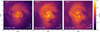 |
Fig. A.2 AB Aur Uφ images in J, H, and Ks bands in a 3″ × 3″ field of view as obtained in P108. The color bar reports the contrast obtained by normalizing with the out of mask PSF image and is displayed in logarithmic scale. North is up and east is left. |
Appendix B Dynamical analysis
Appendix B.1 Dynamics of the spiral arms in the disk
We repeated the analysis of section 2.4 to estimate the rotation of the disk between the three epochs, but focusing on the main spiral arms and the bridge. In Fig. B.1, we present the results for five different masks. As for the spiral S1, the mask S1a includes the feature f1 and the brightest part of S1, while the mask S1b excludes f1 but extend to the northern part of the spiral. For what concern S2, similarly, we considered two masks, S2a located at the brightest northern tip, and S2b which follows S2a all the way to the southern part. The last mask is encompassing the bridge only.
Appendix B.2 Dynamics of the features
Further analysis of the dynamics of the features requires to explore more orbital solutions, in particular those that are out of the disk plane. To account for such solutions, we use the package orbitize! (Blunt et al. 2020). Measuring precisely the position of the features is a complicated task, the Gaussian fitting being systematically biased by the other surrounding spiral features as well as the evolution of the feature themselves (see Fig. 5). Therefore, we proceed with a coarse visual centroiding, assigning a conservative error bar of 10 mas per axis (about 1 pixel). These astrometric measurements for f1, f2, and f3 are provided in Tab. B.1. For f2, this is in good agreement with Gaussian fitting within error bars, while because of the above mentioned biases, for f3, and particularly f1 (since the feature is extended) this is more discrepant. Because of the small orbital coverage and the few data points, we opt for the OFTI method instead of MCMC as it is more relevant in that particular case (Blunt et al. 2017). In addition, we impose prior constraints, restricting the eccentricity to a range of 0.0 – 0.3 with a uniform distribution (to minimize biases), leaving the other parameters free. The results are shown in Fig. B.2 and Fig. B.3. Interestingly, even if the orbit sampling is very poor, we note that the orbits of the three features have their inclination from the sky plane peaking at about 50° – 52° for f1 and f2, and 57° for f3, but with large dispersion of typically ±20°. Calculating the mutual inclinations, φ, with the disk plane requires to take into account the position angle of the disk, Ωd, and the position angle of the nodes of the features’ orbits, Ωf, as well as the inclination of the planes, id and if, as follows:
 (B.1)
(B.1)
As seen in the corner plots (Fig. B.3) the orbital fits provide systematically two solutions for Ωf which differ by ~ 180°. The corresponding mutual inclinations for f1, f2, and f3 are : 75°, 38°, 34°, or 32°, 77°, 78°. Although, the posterior distributions of the inclinations are rather broad, the mutual inclinations would always be larger than ≳ 15°, so not compatible with perfectly coplanar orbits. Furthermore, this experiment shows that the apparent stability of f2 can be interpreted as an object orbiting out of the disk plane.
Astrometry of f1, f2 and f3.
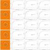 |
Fig. B.1 Same as Fig. 4 for the various masks for the spirals and the bridge shown in the left column: from top to bottom: S1a, S1b, S2a, S2b, and the bridge. |
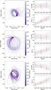 |
Fig. B.2 Orbital solutions displayed in the sky plane, calculated with orbitize!, for f1, f2 and f3 (top to bottom). |
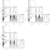 |
Fig. B.3 Posterior distributions for the semi-major axis (a1), the position angle of the ascending node (Ω1), and the inclination (inc1) of the orbital solutions, calculated with orbitize!, for f1 (top left), f2 (top right) and f3 (bottom left). |
Appendix C Width of radial shadows
With the objective of understanding whether the shadows could have a planetary origin, we compare the width of the shadow with the predictions of the model by Akansoy et al. (2025). A shadow cast by a planet is expected to be thinner than shadows due to an inclined inner disk. Similarly to section 2.4 we perform the analysis in the disk plane, using both the images of Fig. 6 (Nov. 25th, 2021), and the PCA (PC#2, Fig. 7). We focus on the two main shadows sh1 and sh2 (respectively oriented at PA ≈ 275° and PA ≈ 348° in the sky plane) since they are sufficiently well visible. We use a rectangular aperture to isolate the shadows from 33 to 74 pixels in the deprojected image coordinates (corresponding to physical distances of ~64 to 144 au), with a width of 16 pixels (~31 au), and fit a Gaussian profile perpendicularly to the shadow. Then, to reproduce the findings of Akansoy et al. (2025) the width is converted to an angle and scaled with the ratio of the Hill’s radius of a planet to the distance of the planet, which corresponds to a factor (Mp/3M*)−1/3. We assume an object of 30 Mjupiter (but the dependence with the mass is small). The results are presented in Fig. C.1. Although it is difficult to match our width measurements with the model, we end up with values that are qualitatively consistent with those presented in Akansoy et al. (2025) (their Fig. 7). Therefore, this exercise demonstrates the difficulty to measure the width of a shadow and to unambiguously connect this value to the mass of the source casting the shadow.
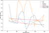 |
Fig. C.1 Angular width of the shadows sh1 (orange line) and sh2 (blue line) versus the separation to star, measured in the disk plane for the second epoch in H band (Nov. 25th, 2021, solid lines) and the second principal component (dashed lines), compared to Akansoy et al. (2025). |
Appendix D ZIMPOL data reduction
In this section, we present the raw PSFs and coronagraphic images (Fig. D.1), the measured contrasts (Fig. D.2), and the on-sky transmission of the coronagraphic mask (Fig. D.3).
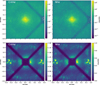 |
Fig. D.1 PSFs (log scale) and raw coronagraphic (linear scale) images with ZIMPOL in both filters CntHα and N_Hα. The field of view is 0.8″ × 0.8″. Intensities are in counts per second. Corresponding contrasts are plotted in Fig. D.2. |
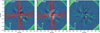 |
Fig. D.3 Traces of the spiders coronagraphic mask during the observation (red shaded area) superimposed with the image in filters CntHα (left) and N_Hα (middle). For comparison we also display the N_Hα alone (right), and the contours of the J band image (middle). |
Appendix E ZIMPOL Hα photometry
Appendix E.1 Self-subtraction in ZIMPOL ADI images
The features we are interested in to derive the photometry, in particular f1, the bridge and AB Aur b, undergo self-subtraction due to the ADI processing. In contrary to a point source, the self-subtraction of an extended source cannot be fully predicted because it depends on the morphology of the source which itself is modified by the self-subtraction. Here, we proceed with a forward modeling approach which applies the very same principal components calculated for the data onto the model image. We assume each feature to be a Gaussian 2D function and we derive the flux ratio before and after the ADI processing in the same apertures used for the photometry. The size of the Gaussian and the amplitude of the self-subtraction (τ) are provided below:
f1: 35 × 123 mas, τ = 3.75
bridge: 123 × 53 mas, τ = 4.3
f1 knot: 7 × 7 mas, τ = 2.37
ABAur b: 90 × 60 mas, τ = 1.44
An example is shown in Fig. E.1
Appendix E.2 Flux in Hα
To derive thoroughly the Hα emission we follow the method exposed in Cugno et al. (2019), instead of using the ASDI image from Fig. 8. It also relies on the calibration of ZIMPOL zero points carried out by Schmid et al. (2017). The principle is to measure the count rates (cts) of a particular feature in the image, then to convert it to flux (erg/s/cm2) for both filters, and to estimate the contribution of the continuum emission in the Hα filter to derive only the flux in the emission line. The latter is the relevant for estimating the accretion luminosity and the mass accretion rate. We describe below the generic approach, in which we first estimate the flux in the two filters according to Eq. 4 of Schmid et al. (2017) :
 (E.1a)
 (E.1b)
where Czpcnt and Czpline are the zero points in the continuum and in the line, tabulated in Schmid et al. (2017). The extinction parameter k varies with wavelength and was measured for Paranal to be 0.085 mag/airmass, respectively 0.082 mag/airmass, for filters CntHα, respectively NHα. The airmass is on average 1.85 for PSF observations, and 1.84 for coronagraphic observations. The parameter mmode is a transmission correction factor which depends on the dichroic between the science path and the AO path (−0.23 mag for DIC_HA). To estimate the count rate due to the continuum inside the NHα filter, we use Eq. 2 from Cugno et al. (2019) which renormalizes the count rate in CntHα to the zero point of the continuum in NHα :
 (E.2)
(E.2)
and then subtracting the count rate of the continuum to the total count rate in the NHα filter yields:
 (E.3)
(E.3)
We can estimate the line to continuum ratio as ctsHα/ctsNHα.
Then, by analogy with Eq. E.1b the flux of the Hα line reads:
 (E.4)
(E.4)
Appendix E.3 Hα accretion models
For each accretion model the accretion luminosity Lacc relates to the Hα luminosity in a log-log relationship (Fig. E.2), that is either an experimental result or a theoretical result, as follows:
 (E.5a)
 (E.5b)
 (E.5c)
We note that the dispersions of the accretion luminosity calculated from the Hα luminosity is not estimated the same way for the three cases. Equation E.5c stands for a specific composition which has a gas-to-dust ratio of 100, and a dust mixture of 40% silicates + 40% water-ice + 20% carbon, and a grain size of 1 μm, but it has been also derived for 3 other compositions with different coefficients (see Tables 3 and 4 in Szulágyi & Ercolano 2020). For each mixture the coefficients can also vary depending on the planet position on its orbit.
Photometry and accretion rate. Fluxes are in erg/s/cm2, luminosities in L⊙, accretion masses in MJup/yr and masses in MJup.
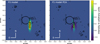 |
Fig. E.1 Forward modeling of f1: a Gaussian features matching f1 size (left) and the corresponding image with PCA (right). Black contours depict the NHα PCA image, and the photometric aperture is also indicated in white. |
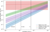 |
Fig. E.2 Comparison of models (Szulágyi & Ercolano 2020; Aoyama et al. 2021a; Rigliaco et al. 2012; Alcalá et al. 2017) predicting the accretion luminosity as a function of the Hα luminosity. Vertical lines stand for the luminosity measured for AB Aur b, f1, and the knot. |
All Tables
Photometry and accretion rate. Fluxes are in erg/s/cm2, luminosities in L⊙, accretion masses in MJup/yr and masses in MJup.
All Figures
|
Fig. 1 H-band images of AB Aur Qφ in a 3″ × 3″ field of view at three epochs (December 2019, November 2021, and October 2023). The top row is displayed in logarithmic scale, while the bottom row is a high-pass filtered version in linear scale. The color bar shows the contrast obtained by normalizing with the out-of-mask point spread function image. North is up and east is left. |
| In the text | |
|
Fig. 2 H-band images of AB Aur (October 2023), showing the main structures. Top panel: scattered light features. Bottom panel: millimetric features (yellow: dust ring; white: 12CO spirals S1 and S2 from Tang et al. (2017); green: SO ring and SO peak from Dutrey et al. (2024); blue: C18O ring from Dutrey et al. (2024) and pink: out of plane spirals (or streamers) St1, St2, and St3 from Speedie et al. (2025). The central yellow cross indicates the star’s position. Images are normalized by r2 and spatially filtered. North is up and east is left. |
| In the text | |
|
Fig. 3 H-band images of AB Aur at three epochs in a 1″ × 1″ field of view. The rightmost panel displays the contours of epoch 1 (dashed line) and epoch 3 (solid line) superimposed on the image from epoch 3. Images are spatially filtered. North is up and east is left. |
| In the text | |
|
Fig. 4 Disk rotation as a function of radius for each pair of epochs. The data points are shown in red, while the blue line represents the expected Keplerian rotation in the disk plane (solid) and for inclinations of 20°, 30°, 40°, and 50° (darkest to lightest lines). The residuals between the data and the Keplerian are shown below each plot. From top to bottom: Epoch 2 vs. epoch 1, epoch 3 vs. epoch 2, and epoch 3 vs. epoch 1. The time interval is given in years. |
| In the text | |
|
Fig. 5 Rotation of the main disk features for two epoch pairs (2021 vs. 2019 in blue and 2023 vs. 2019 in red). The symbols correspond to f1 (circle), f2 (diamond), f3 (square), and the bridge (triangle). Each curve shows the expected Keplerian rotation using the same color coding as the symbols. The left panel shows the results from the optimization method, while the right panel shows results from Gaussian fitting (only for f1, f2, and f3). |
| In the text | |
|
Fig. 6 Deprojected H-band images of AB Aur for the three epochs. Dotted lines approximately trace the main shadow patterns identified at each epoch. Images are multiplied by r2 and spatially filtered. The blue, green, and pink circles trace the potential location of clumps that could be casting the shadows. |
| In the text | |
|
Fig. 7 Principal component analysis (PCA) of the three images shown in Fig. 6. Principal components 0, 1, and 2 are shown from left to right. The shadow positions at the first epoch (December 18, 2019) are superimposed. |
| In the text | |
|
Fig. 8 Principal component analysis (PCA) reduction in ADI using ZIMPOL for the two filters CntHα (left) and N_Hα (middle and right). The rectangle indicates the aperture used for photometry. Structures oriented along the diagonal of the images at about 0.35″ from the star are produced by the SPHERE deformable mirror (DM). The right subpanel shows the IRDIS DPI J-band contours overlaid on the ZIMPOL NHα PCA image. The intensity scale is in contrast relative to the star. North is up and east is left. |
| In the text | |
|
Fig. 9 Images in NHα (left), with a fake planet (FP) injected at the flux of AB Aur b (middle) and with twice the flux (right). Labels indicate the position of the candidate planet. The dashed circles trace the region contaminated by the AO correction radius, while the pink cross represents the companion candidate reported in Kozdon et al. (2026) in 12CO ro-vibrational transitions. The yellow circle at ρ = 0.35″, PA = 119.7° marks a new signal that remains to be investigated. |
| In the text | |
|
Fig. 10 GaiaPMEX analysis for AB Aur showing the solutions (green shades) at 1, 2 and 3 σ in a mass/semi-major axis (sma) diagram. |
| In the text | |
|
Fig. A.1 Same as Fig. 1 but at one period of observations (Nov. 2021 through Jan. 2022) and for the J, H and Ks bands. For visualisation purpose the contrasts of the J and K bands were renormalized to that of the H band. |
| In the text | |
|
Fig. A.2 AB Aur Uφ images in J, H, and Ks bands in a 3″ × 3″ field of view as obtained in P108. The color bar reports the contrast obtained by normalizing with the out of mask PSF image and is displayed in logarithmic scale. North is up and east is left. |
| In the text | |
|
Fig. B.1 Same as Fig. 4 for the various masks for the spirals and the bridge shown in the left column: from top to bottom: S1a, S1b, S2a, S2b, and the bridge. |
| In the text | |
|
Fig. B.2 Orbital solutions displayed in the sky plane, calculated with orbitize!, for f1, f2 and f3 (top to bottom). |
| In the text | |
|
Fig. B.3 Posterior distributions for the semi-major axis (a1), the position angle of the ascending node (Ω1), and the inclination (inc1) of the orbital solutions, calculated with orbitize!, for f1 (top left), f2 (top right) and f3 (bottom left). |
| In the text | |
|
Fig. C.1 Angular width of the shadows sh1 (orange line) and sh2 (blue line) versus the separation to star, measured in the disk plane for the second epoch in H band (Nov. 25th, 2021, solid lines) and the second principal component (dashed lines), compared to Akansoy et al. (2025). |
| In the text | |
|
Fig. D.1 PSFs (log scale) and raw coronagraphic (linear scale) images with ZIMPOL in both filters CntHα and N_Hα. The field of view is 0.8″ × 0.8″. Intensities are in counts per second. Corresponding contrasts are plotted in Fig. D.2. |
| In the text | |
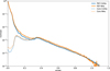 |
Fig. D.2 Contrasts measured for the PSF and coronagraphic images displayed in Fig. D.1. |
| In the text | |
|
Fig. D.3 Traces of the spiders coronagraphic mask during the observation (red shaded area) superimposed with the image in filters CntHα (left) and N_Hα (middle). For comparison we also display the N_Hα alone (right), and the contours of the J band image (middle). |
| In the text | |
|
Fig. E.1 Forward modeling of f1: a Gaussian features matching f1 size (left) and the corresponding image with PCA (right). Black contours depict the NHα PCA image, and the photometric aperture is also indicated in white. |
| In the text | |
|
Fig. E.2 Comparison of models (Szulágyi & Ercolano 2020; Aoyama et al. 2021a; Rigliaco et al. 2012; Alcalá et al. 2017) predicting the accretion luminosity as a function of the Hα luminosity. Vertical lines stand for the luminosity measured for AB Aur b, f1, and the knot. |
| In the text | |
Current usage metrics show cumulative count of Article Views (full-text article views including HTML views, PDF and ePub downloads, according to the available data) and Abstracts Views on Vision4Press platform.
Data correspond to usage on the plateform after 2015. The current usage metrics is available 48-96 hours after online publication and is updated daily on week days.
Initial download of the metrics may take a while.