| Issue |
A&A
Volume 631, November 2019
|
|
|---|---|---|
| Article Number | A84 | |
| Number of page(s) | 9 | |
| Section | Stellar structure and evolution | |
| DOI | https://doi.org/10.1051/0004-6361/201936510 | |
| Published online | 24 October 2019 | |
Detection of Hα emission from PZ Telescopii B using SPHERE/ZIMPOL⋆
1
Max Planck Institute for Astronomy (MPIA), Königstuhl 17, 69117 Heidelberg, Germany
e-mail: This email address is being protected from spambots. You need JavaScript enabled to view it.
2
ETH Zürich, Institute for Particle Physics and Astrophysics, Wolfgang-Pauli-Str. 27, 8093 Zürich, Switzerland
3
Center for Theoretical Astrophysics and Cosmology, Institute for Computational Science, University of Zürich, Winterthurerstrasse 190, 8057 Zürich, Switzerland
4
Univ. Grenoble Alpes, CNRS, IPAG, 38000 Grenoble, France
Received:
14
August
2019
Accepted:
16
September
2019
Abstract
Hα is a powerful tracer of accretion and chromospheric activity, which has been detected in the case of young brown dwarfs and even recently in planetary mass companions (e.g. PDS70 b and c). Hα detections and characterisation of brown dwarf and planet companions can further our knowledge of their formation and evolution, and expanding such a sample is therefore our primary goal. We used the Zurich Imaging POLarimeter (ZIMPOL) of the SPHERE instrument at the Very Large Telescope (VLT) to observe the known 38−72 MJ companion orbiting PZ Tel, obtaining simultaneous angular differential imaging observations in both continuum and narrow Hα band. We detect Hα emission from the companion, making this only the second Hα detection of a companion using the SPHERE instrument. We used our newly added astrometric measurements to update the orbital analysis of PZ Tel B, and we used our photometric measurements to evaluate the Hα line flux. Given the estimated bolometric luminosity, we obtained an Hα activity (log(LHα/Lbol)) between −4.16 and −4.31. The Hα activity of PZ Tel B is consistent with known average activity levels for M dwarf of the same spectral type. Given the absence of a known gaseous disk and the relatively old age of the system (24 Myr), we conclude that the Hα emission around PZ Tel B is likely due to chromospheric activity.
Key words: instrumentation: high angular resolution / methods: observational / stars: activity / stars: individual: PZ Tel / stars: imaging
ESO programme ID: 0101.C-0672(A); P.I.: A. Musso Barcucci. The reduced data products are available via ESO/phase 3.
© A. M. Barcucci et al. 2019
 Open Access article, published by EDP Sciences, under the terms of the Creative Commons Attribution License (http://creativecommons.org/licenses/by/4.0), which permits unrestricted use, distribution, and reproduction in any medium, provided the original work is properly cited.
Open Access funding provided by Max Planck Society.
1. Introduction
Hα emission from low-mass stars and brown dwarfs can have multiple origins. In the case of young objects (< 10 Myr) gas from the circumstellar disk can be accreted onto a circumsecondary disk and, due to the high temperatures of the shock front, this can lead to dissociation of H2 molecules and consequent Hα emission (Szulágyi & Mordasini 2017). In the case of young non-accreting stars, chromospheric activity produces well-known emission lines, with Hα being one of the most prominent ones.
Hα emission from single low-mass stars and brown dwarfs has been extensively studied through the years. West et al. (2004) used around 8000 single M dwarf spectra from the Sloan Digital Sky Survey (SDSS) to evaluate their Hα flux and investigate the activity fraction and strength as a function of spectral type. They quantified the activity as logarithm of the ratio between the Hα luminosity and bolometric luminosity, and they found a peak in the fraction of active stars around spectral type M8, where more than 70% of stars were active. They also evaluated the mean activity strength as the ratio between the Hα luminosity, and the bolometric luminosity finding that it is constant between M0 and M5 and that it declines at later spectral types. Similar trends were recovered by subsequent surveys: Lee et al. (2009) studied the short-term Hα variability of 43 single M dwarf, finding a similar decrease in the activity strength for later spectral types, as well as an increase in the variability level up to spectral type M7. Kruse et al. (2010) also focused on short-timescale Hα variability using nearly 53 000 spectra from SDSS; they recovered both the log(LHα/Lbol) activity trend (that increases until ∼M6 with subsequent decrease) and the same variability trend (that increases with later spectral type). More recently, Robertson et al. (2013) studied the correlation between activity, mass, spectral type, and metallicity of 93 stars ranging from K5 to M5. They find that the activity trend is recovered and, at a given stellar mass, metal rich stars appear to be more active.
However, much less is known about the Hα emission from companions in binary systems, the main reason being the difficulty in disentangling the two components in the spectrum (with few exceptions, see e.g. Bowler et al. 2014, Santamaría-Miranda et al. 2018). Few remarkable Hα detections, often associated with accretion, have been made using high-contrast imaging techniques, which allow to differentiate between the two components in a binary system and evaluate the Hα flux from the companion. One example is HD 142527 B, an accreting M-dwarf companion first detected in Hα by Close et al. (2014) with the Magellan Adaptive Optics system (MagAO). The companion is later re-detected using the Zurich Imaging POLarimeter (ZIMPOL) of the SPHERE instrument at the Very Large Telescope (VLT) by Cugno et al. (2019), who also searched for local accretion signals in other objects suspected of hosting forming giant planets. More recently, Wagner et al. (2018) claim the detection of Hα emission from the young planet PDS 70 b. Haffert et al. (2019) were also able to detect Hα emission from PDS 70 b with the MUSE Integral Field Spectrograph at the VLT (Bacon et al. 2010) and identified another accreting protoplanet in the same system, PDS 70 c. Sallum et al. (2015) claimed to have detected accretion from the companion orbiting around LkCa 15, but recent studies from Thalmann et al. (2016) and Currie et al. (2019) could not confirm it, also doubting whether the companions exist at all. Other remarkable Hα detections include GQ Lup b and DH Tau b, both detected by Zhou et al. (2014) using the Hubble Space Telescope, and three newly detected brown dwarf companions from the Upper Sco region (Petrus et al. 2019).
These detections are fundamental for various reasons: firstly, they prove that it is feasible to detect planets and low-mass stellar companions using Hα emission as a tracer; secondly, they give initial insight into the gas-accretion phase of planet and brown dwarf formation; and thirdly, they show that it is possible to use state of the art high contrast imaging instruments and techniques to detect Hα emission in binary systems.
In order to learn more about the early stages of planet formation and evolution, increasing the number of directly imaged known companions with Hα detection is our primary goal. In this work, we present SPHERE/ZIMPOL angular differential imaging (ADI; Marois et al. 2006) observations in Hα of the known companion orbiting around the star PZ Tel. In Sect. 2 we present the target and in Sect. 3 we detail the observations and data reduction; we present the analysis and the results in Sect. 4 and we summarise our conclusions in Sect. 5.
2. PZ Tel B
PZ Tel (HD 174429, HIP 92680) is a G6.5 type star with an age of 24 ± 3 Myr (Jenkins et al. 2012, Bell et al. 2015), belonging to the β Pic moving group (Zuckerman et al. 2001) at a distance of ∼47 pc (Gaia Collaboration 2018). In 2010, two independent studies discovered a sub-stellar companion at a separation of ∼0.3 arcsec: Mugrauer et al. (2010) with the NaCo instrument at the VLT and Biller et al. (2010) with the Near-Infrared Coronagraphic Imager (NICI) at Gemini South. Both authors interpolated low-mass objects evolutionary tracks (Baraffe et al. 2002) and inferred a mass of  and 36 ± 6 MJ, which corresponds to a spectral type of M5−9. Following its discovery, the PZ Tel system has been the subject of several studies. Jenkins et al. (2012) use spectra obtained with the Fiber-fed Extended Range Optical Spectrograph (FEROS) to derive a rotational velocity of the host star of v sin i = 73 ± 5 km s−1, a metallicity of [Fe/H] = 0.05 ± 0.20 dex, and an age of 5−27 Myr which led to a revised mass for PZ Tel B of 62 ± 9 MJ via comparison with evolutionary models. Additional spectroscopic information was obtained with the Spectrograph for INtegral Field Observations in the Near Infrared (SINFONI) at the VLT (Schmidt et al. 2014), leading to a mass estimate for the companion of
  , and a bolometric luminosity of
  , which are independent of both age and evolutionary model used. More recently, Maire et al. (2016) obtained multi-band photometric observations of the companion using the InfraRed Dual-band Imager and Spectrograph (IRDIS), the Integral Field Spectrograph (IFS), and ZIMPOL at VLT/SPHERE, and derived a mass of 38−72 MJ (spectral type M7 ± 1), which we use in this work. The observed mean activity strength value for this spectral type are −4.31 according to West et al. (2004), and −4.37 according to Kruse et al. (2010). Maire et al. (2016) also derived a bolometric luminosity for the companion of log(Lbol/L⊙) = − 2.51 ± 0.10. Riviere-Marichalar et al. (2014) obtained Herschel-PACS far-IR photometric observations at 70, 100, and 160 μm of 19 β Pic moving group members. They were able to exclude the presence of a substantial debris disk around PZ Tel, due to the non-detection of excess in the aforementioned bands, placing an upper limit on the infrared excess of LIR/L⋆ < 2.3 × 10⁻⁵. Table 1 summarises the host star and companion properties.
Fundamental parameters and properties of the PZ Tel system.
3. Observations and data reduction
We observed the PZ Tel system with the ZIMPOL instrument at VLT/SPHERE (Schmid et al. 2018), obtaining simultaneous coronagraphic ADI observations in the Cnt_Hα and NHα filter. The data were taken on UT 2018-05-30 in two observation blocks before and after the meridian passage, to maximise the total field rotation while allowing flexibility in the observing schedule. Each observing block consists of a set of science exposures with an integration time of 220 s, which were bracketed with non-saturated observations of the star with DIT = 52 seconds, that we denote as flux frames. We also recorded a centre frame at the beginning and end of each observing block, in which a pattern is applied to the deformable mirror creating 4 bright copies of the central PSF outside of the coronagraph (in a symmetric pattern around the central star) which are used to compute the stellar position behind the coronagraph. The conditions were clear throughout the entire observations, with a median DIMM seeing of 0.9 arcsec. Standard bias, dark and flat calibrations were observed on the same night. Details of the observations, as well as main ZIMPOL detector characteristics, are summarised in Table 2.
Summary of observations and detector characteristics.
The data was reduced using the ZIMPOL reduction pipeline developed and maintained at ETH Zürich which consists of: flat fielding, bias correction and dark subtraction, remapping the initial 7.2 × 3.6 mas pix−1 platescale into the squared grid of 3.6 × 3.6 mas pix−1, and separating the frames in the two filters. The pipeline was applied to the flux, centre, and science frames. To account for possible shifting of the stellar position on the detector during the observations, we fitted a two dimensional gaussian to each spot in the 4 cosmetically reduced centring frames (and in both filters), computing the centre as intersection of the connecting lines. The final centre and relative error are the mean and standard deviation of these 4 centres (for each filter). We then re-centre the science frames using the scipy.ndimage.interpolation.shift package with spline interpolation of order 3, and cut them to stamps of 1.62 × 1.62 arcsec ending up with 20 cosmetically reduced and centred science frames for each filter. Since the unsaturated star is offset from the coronagraph and therefore visible, we fitted a two dimensional gaussian to re-centre the flux frames, ending up with eight cosmetically reduced and centred flux frames for each filter. The parallactic angle for each frame is automatically computed by the ZIMPOL pipeline, and takes care of a constant known offset of 134 ± 0.5° (Maire et al. 2016; Cugno et al. 2019) for which the frames must be rotated in the counterclockwise direction.
4. Analysis and results
The goal of this paper is to detect and quantify Hα emission from the companion around PZ Tel, to expand the sample of known brown dwarfs and planetary companions with Hα detection and better understand the formation and evolution of these objects. We also provide an additional astrometric measurement of the PZ Tel B, extending the time baseline by four more years. We clearly detected the companion in both Cnt_Hα and NHα filter, as shown in Fig. 1. Even though the detection is clear in both filters, we also analysed the data with angular spectral differential imaging (ASDI) technique, shown in the rightmost panel of Fig. 1. We refer to Appendix A, as well as Cugno et al. (2019), for a detailed explanation of the ASDI analysis.
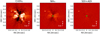 |
Fig. 1. Reduced images showing PZ Tel B. In all three images the green cross marks the position of the central star, the data is oriented with north up, and the companion is clearly visible NE of the star. The images are normalised and the colour map was chosen for a better visualisation of the data. left panel: classical ADI reduced image of the continuum Hα filter frames. Central panel: classical ADI reduced image of the narrow band Hα filter frames. Right panel: ASDI analysis. |
4.1. Astrometry and flux contrast
We quantified the astrometry and flux contrast of the companion, for both filters, using the ANDROMEDA package (Cantalloube et al. 2015). This algorithm needs as input the cosmetically reduced frames, the corresponding parallactic angles, and an unsaturated PSF of the central star to be used as template to create and inject fake negative companions. We created this unsaturated image of the host star (for both filters) as median combination of all the flux frames, scaled to the DIT of the science frames. We set the Inner Working Angle parameter to 1.0 λ/D (we refer to the ANDROMEDA paper for a detailed explanation of how the package works). The astrometry and flux contrast evaluated with ANDROMEDA are presented in Table 3.
Astrometry and flux contrast evaluated with ANDROMEDA, for both continuum and narrow band filter.
4.2. Photometry
We followed the prescriptions from Cugno et al. (2019) to convert the flux contrasts into physical fluxes for both filters. The only difference was that, due to the presence of the coronagraph, we evaluated the flux of the host star using the flux frames instead of the science frames. Given the vicinity of the bands, we assumed that the continuum flux density is the same in both filters and we evaluated the flux in both. We then used the continuum flux density to evaluate the contamination of the narrow band filter due to continuum emission, and we corrected for it, obtaining the Hα line flux. We refer to Appendix B for a detailed step-by-step description of the analysis (we also performed an alternative photometric analysis described in Appendix C). After correcting for extinction (see Appendix B and Table 1), the total flux in the continuum filter, the total flux in the narrow band filter and the line flux, are:
We now have the flux of the primary in the two filters and, together with the companion flux contrast (see Table 3), we can calculate the companion flux in both bands. The companion line flux is then the difference between the fluxes in the two filters (normalising the continuum flux to the width of the Hα filter). The final values for the companion are:
The companion Hα line flux can be converted into a luminosity, multiplying by the squared distance, obtaining:

Finally, we can evaluate the Hα activity as the ratio between the Hα luminosity and the bolometric luminosity of the object. For a bolometric luminosity of PZ Tel B of log10(Lbol/L⊙) =  (Schmidt et al. 2014), we obtain an Hα activity of log10(LHα/Lbol) = − 4.16 ± 0.08. Similarly, we obtain log10(LHα/Lbol) = − 4.31 ± 0.1 in the case of log10(Lbol/L⊙) = −2.51 ± 0.10 (Maire et al. 2016). The Hα activity values agree within the errorbars.
4.3. Orbital constraints
Following its discovery in 2010, PZ Tel B has been observed several times in the last years, providing various astrometric measurements on an increasingly large time baseline. We compiled all the available astrometric datapoints from the literature in Table 4 and we show the position angle and separation of the companion through time in Fig. 2. With our newly added observations, the available baseline is now ∼12 yr. Mugrauer et al. (2012) were the first to report a deceleration of the variation of the angular separation of the companion, to be expected for an object moving on a Keplerian orbit towards apastron, which would support a bound orbit solution. Deceleration was also detected by Ginski et al. (2014) and Maire et al. (2016). We revisited the literature data and, together with our newly added astrometry, we further confirm this trend. The angular separation increases with a rate of dsep/t = 35.3 ± 1.2 mas yr−1 between June 2007 and September 2009, and then of 32.9 ± 1.6 mas yr−1 between September 2009 and September 2010. The rate keeps decreasing all the way down to 27.7 ± 0.6 mas yr−1 between June 2012 and July 2014 and, finally, of just 23.0 ± 0.3 mas yr−1 between July 2014 and May 2018. Given the deceleration of the companion, we decided to restrict the following orbital analysis to bound orbits only (e ≤ 1).
Astrometric measurements for PZ Tel B available in the literature.
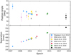 |
Fig. 2. Separation and position angles of PZ Tel B, at various epochs. We show the astrometric values found in the literature (see Table 4) in various colours, together with the astrometry presented in this paper, for both filters (black points). |
Given the newly extended astrometric baseline, we explored the possible orbital solutions using the Python package PyAstrOFit1 (Wertz et al. 2017) which provides a series of tools to fit orbits using the emcee package (Foreman-Mackey et al. 2013) with the modified Markov chain Monte Carlo (MCMC) approach described in Goodman & Weare (2010). We assumed uniform prior distribution for the semi-major axis (a), the eccentricity (e), the inclination (i), the longitude of ascending node (Ω) and argument of periapsis (ω), and the time of periastron passage (tp). Assuming a system mass of 1.2 M⊙ (see Table 1), we explored all possible bound solutions (e ≤ 1), allowing a range of semi-major axis between 10 and 1200 au, an inclination between 10 and 180°, and Ω and ω within natural boundaries. The only other hyperparameters are the number of walkers (which we set to 1200), and the scale parameter a, which directly impacts the acceptance rate AR (Mackay 2003) of the walkers. We manually tuned a to ensure an AR between 0.2 and 0.5. PyAstrOFit relies on the Gelman Rubin  statistical test to check for convergence (Gelman & Rubin 1992; Ford 2006), which is considered reached when all the parameters pass the test three times in a row (with a threshold of
  , where the closer the
  value is to 1 the closer the Markov chain is to convergence).
The posterior distributions of the orbital elements, as well as the correlation between them, is shown in the corner plot of Fig. 4. The eccentricity distribution shows two peaks at ∼0.55 and at 1, which is a lower boundary smaller than what found by previous studies (0.62 < e < 0.99 in Ginski et al. (2014) and e ≳ 0.66 in Maire et al. (2016)) and significantly smaller than the lower boundary of 0.91 found in the most recent orbital study of PZ Tel B, by Beust et al. (2016). A possible explanation for this difference lies in the different boundaries applied: Beust et al. (2016) allowed not-bound orbits while in this work we only considered orbits with e < 1. Our best solution for the semi-major axis of 31.3 au agrees with previous works (17.86 < a < 1098 au in Ginski et al. 2014 and a ≳ 24.5 au in Maire et al. 2016). We found a best inclination of 91.6 degrees, which is in agreement with previous ranges of 91.3 ° < i < 168.1° for Ginski et al. (2014) and 91 ° < i < 96.1° for Maire et al. (2016). Previous confidence intervals for the longitude of ascending node were 50 ° < Ω < 70° for Ginski et al. (2014) and 55.1 ° < Ω < 59.1° for Maire et al. (2016), and Ginski et al. (2014) cited an interval of 122.2 ° < ω < 306° for the argument of periapsis. All of these agree with our best solutions of Ω = 58.8° and ω = 239.2°. The best solution for the time of periastron passage corresponds to 1996.3, which agrees within the confidence intervals of previous works, but it is systematically lower than their best solutions (2002.9 for Mugrauer et al. 2012, 2003.5 for Ginski et al. 2014 and 2002.5 for Beust et al. 2016).
The best solutions in terms of reduced χ2 and the 1-σ confidence intervals are reported in Table 5. The orbit corresponding to these best parameters is shown in Fig. 3, where we overplot the astrometric points (both from literature and from this work) as well as the position of the host star, the direction of the ascending node and the position of periapsis.
Best solutions in terms of reduced χ2 and 1-σ confidence intervals for all the orbital elements.
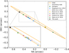 |
Fig. 3. Best orbital solution found with PyAstrOFit. The orange line shows the orbit, the yellow star marks the position of the primary and the various astrometric measurements are shown with the same colour coding of Fig. 2. The green square marks the position of the periapsis, and the dashed black line shows the position of the ascending node. |
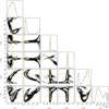 |
Fig. 4. Posterior distributions of the orbital elements (diagonal panels) and correlation between the parameters (off-axis panels). The orange lines and squares mark the position of the best solution found in terms of reduced χ2, as reported in Table 5. |
Our new astrometric datapoints are in agreement with previous measurements in terms of orbital elements, and help to tighten the uncertainties.
5. Discussion and conclusions
We presented SPHERE/ZIMPOL observations of the known sub-stellar M dwarf companion around PZ Tel, taken in both Hα continuum and narrow band filter. We detected the companion in both datasets obtaining new astrometric and photometric measurements. This currently represents the second only Hα detection of a companion using the SPHERE instrument, and it further proves the capability of this instrument to detect Hα signatures in binary systems.
We used our newly added astrometric data, together with values from the literature, to explore the allowed orbital solutions for PZ Tel B, finding orbital elements in agreement with what done in previous works (with the only exception being our lower boundary on the eccentricity). Our added data extends the available baseline for orbital studies of PZ Tel B up to ∼12 yr. We find that the companion is clearly decelerating over time, which is to be expected for a Keplerian bounded object moving towards apastron. We evaluated the Hα luminosity and activity of PZ Tel B, finding values for log10(LHα/Lbol) of −4.16 ± 0.08 and −4.31 ± 0.10, for bolometric luminosities of −2.66 and −2.51, respectively.
Several studies investigated the Hα activity in M dwarf, both as a function of spectral type and mass. West et al. (2004) evaluated the average Hα activity as a function of spectral type, finding an average activity of −4.0, −4.31 and −4.10 for spectral types of M6, M7 and M8, respectively. A later study from Kruse et al. (2010) found similar average activity levels of −3.89, −4.35 and −4.17 for the same spectral types. Based on its spectral type, PZ Tel B thus appears to be slightly less active than the average, while still be consistent with the average values within the uncertainties.
Given the age of the system, and the absence of a known gaseous disk, it is unlikely that the observed Hα luminosity is due to accretion processes. The fact that the activity level is consistent with what is expected for an object of spectral type M6-8, leads us to conclude that the most likely explanation for the Hα luminosity observed in PZ Tel B is chromospheric activity.
Finally, we suggest that a possible explanation for the below average Hα value of PZ Tel B is that the object has a variable emission and we happened to observe it during a moment of low activity. This reasoning is supported primarily by the late spectral type of the object, which is known to correlate with a higher variability level (see, e.g. Kruse et al. 2010); in addition, the companion has a high metallicity, which Robertson et al. (2013) correlated with a higher activity. However, follow-up Hα observations would be needed to establish whether PZ Tel B displays a variable chromospheric activity.
Acknowledgments
Based on observations collected at the European Southern Observatory under ESO programme 0101.C-0672(A). A. M. B. would like to thank the anonymous referee for the useful and constructive comments. J. S. acknowledges the support from the Swiss National Science Foundation (SNSF) Ambizione grant PZ00P2_174115. A. M. acknowledges the support of the DFG priority programme SPP 1992 “Exploring the Diversity of Extrasolar Planets” (MU 4172/1-1 and QU 113/6-1). G. C. and S. P. Q. thank the Swiss National Science Foundation for the financial support under the grant number 200021_169131. This research made use of Astropy (http://www.astropy.org), a community-developed core Python package for Astronomy (Astropy Collaboration 2013, 2018).
References
- Astropy Collaboration (Robitaille, T. P., et al.) 2013, A&A, 558, A33 [NASA ADS] [CrossRef] [EDP Sciences] [Google Scholar]
- Astropy Collaboration (Price-Whelan, A. M., et al.) 2018, AJ, 156, 123 [Google Scholar]
- Bacon, R., Accardo, M., Adjali, L., et al. 2010, in Ground-based and Airborne Instrumentation for Astronomy III, Proc. SPIE, 7735, 773508 [CrossRef] [Google Scholar]
- Baraffe, I., Chabrier, G., Allard, F., & Hauschildt, P. H. 2002, A&A, 382, 563 [NASA ADS] [CrossRef] [EDP Sciences] [Google Scholar]
- Bell, C. P. M., Mamajek, E. E., & Naylor, T. 2015, MNRAS, 454, 593 [NASA ADS] [CrossRef] [Google Scholar]
- Beust, H., Bonnefoy, M., Maire, A. L., et al. 2016, A&A, 587, A89 [NASA ADS] [CrossRef] [EDP Sciences] [Google Scholar]
- Biller, B. A., Liu, M. C., Wahhaj, Z., et al. 2010, ApJ, 720, L82 [NASA ADS] [CrossRef] [Google Scholar]
- Biller, B. A., Liu, M. C., Wahhaj, Z., et al. 2013, ApJ, 777, 160 [NASA ADS] [CrossRef] [Google Scholar]
- Bowler, B. P., Liu, M. C., Kraus, A. L., & Mann, A. W. 2014, ApJ, 784, 65 [NASA ADS] [CrossRef] [Google Scholar]
- Cantalloube, F., Mouillet, D., Mugnier, L. M., et al. 2015, A&A, 582, A89 [NASA ADS] [CrossRef] [EDP Sciences] [Google Scholar]
- Cardelli, J. A., Clayton, G. C., & Mathis, J. S. 1989, ApJ, 345, 245 [NASA ADS] [CrossRef] [Google Scholar]
- Close, L. M., Follette, K. B., Males, J. R., et al. 2014, ApJ, 781, L30 [NASA ADS] [CrossRef] [Google Scholar]
- Cugno, G., Quanz, S. P., Hunziker, S., et al. 2019, A&A, 622, A156 [NASA ADS] [CrossRef] [EDP Sciences] [Google Scholar]
- Currie, T., Marois, C., Cieza, L., et al. 2019, ApJ, 877, L3 [Google Scholar]
- Ford, E. B. 2006, ApJ, 642, 505 [NASA ADS] [CrossRef] [Google Scholar]
- Foreman-Mackey, D., Hogg, D. W., Lang, D., & Goodman, J. 2013, PASP, 125, 306 [CrossRef] [Google Scholar]
- Gaia Collaboration (Brown, A. G. A., et al.) 2018, A&A, 616, A1 [NASA ADS] [CrossRef] [EDP Sciences] [Google Scholar]
- Gelman, A., & Rubin, D. B. 1992, Stat. Sci., 7, 457 [Google Scholar]
- Ginski, C., Berndt, A., Mugrauer, M., et al. 2014, MNRAS, 444, 2280 [NASA ADS] [CrossRef] [Google Scholar]
- Goodman, J., & Weare, J. 2010, Appl. Math. Comput. Sci., 5, 65 [Google Scholar]
- Haffert, S. Y., Bohn, A. J., de Boer, J., et al. 2019, Nat. Astron., 329 [Google Scholar]
- Husser, T.-O., Wende-von Berg, S., Dreizler, S., et al. 2013, A&A, 553, A6 [NASA ADS] [CrossRef] [EDP Sciences] [Google Scholar]
- Jenkins, J. S., Pavlenko, Y. V., Ivanyuk, O., et al. 2012, MNRAS, 420, 3587 [NASA ADS] [Google Scholar]
- Kruse, E. A., Berger, E., Knapp, G. R., et al. 2010, AJ, 722, 1352 [NASA ADS] [CrossRef] [Google Scholar]
- Lee, K.-G., Berger, E., & Knapp, G. R. 2009, AJ, 708, 1482 [NASA ADS] [CrossRef] [Google Scholar]
- Mackay, D. J. C. 2003, Information Theory, Inference and Learning Algorithms (Cambridge: Cambridge University Press), 640 [Google Scholar]
- Maire, A. L., Bonnefoy, M., Ginski, C., et al. 2016, A&A, 587, A56 [NASA ADS] [CrossRef] [EDP Sciences] [Google Scholar]
- Marois, C., Lafreniere, D., Doyon, R., Macintosh, B., & Nadeau, D. 2006, ApJ, 641, 556 [Google Scholar]
- Mugrauer, M., Röll, T., Ginski, C., et al. 2012, MNRAS, 424, 1714 [NASA ADS] [CrossRef] [Google Scholar]
- Mugrauer, M., Vogt, N., Neuhäuser, R., & Schmidt, T. O. B. 2010, A&A, 523, L1 [NASA ADS] [CrossRef] [EDP Sciences] [Google Scholar]
- Patat, F., Moehler, S., O’Brien, K., et al. 2011, A&A, 527, A91 [NASA ADS] [CrossRef] [EDP Sciences] [Google Scholar]
- Petrus, S., Bonnefoy, M., & Henning, T. 2019, A&A, accepted [Google Scholar]
- Racine, R., Walker, G. A. H., Nadeau, D., Doyon, R., & Marois, C. 1999, PASP, 111, 587 [NASA ADS] [CrossRef] [Google Scholar]
- Riviere-Marichalar, P., Barrado, D., Montesinos, B., et al. 2014, A&A, 565, A68 [NASA ADS] [CrossRef] [EDP Sciences] [Google Scholar]
- Robertson, P., Endl, M., Cochran, W. D., & Dodson-Robinson, S. E. 2013, ApJ, 764, 3 [NASA ADS] [CrossRef] [Google Scholar]
- Sallum, S., Follette, K. B., Eisner, J. A., et al. 2015, Nature, 527, 342 [NASA ADS] [CrossRef] [Google Scholar]
- Santamaría-Miranda, A., Cáceres, C., Schreiber, M. R., et al. 2018, MNRAS, 475, 2994 [NASA ADS] [CrossRef] [Google Scholar]
- Schmid, H. M., Bazzon, A., Milli, J., et al. 2017, A&A, 602, A53 [NASA ADS] [CrossRef] [EDP Sciences] [Google Scholar]
- Schmid, H. M., Bazzon, A., Roelfsema, R., et al. 2018, A&A, 619, A9 [NASA ADS] [CrossRef] [EDP Sciences] [Google Scholar]
- Schmidt, T. O. B., Mugrauer, M., Neuhäuser, R., et al. 2014, A&A, 566, A85 [NASA ADS] [CrossRef] [EDP Sciences] [Google Scholar]
- Szulágyi, J., & Mordasini, C. 2017, MNRAS, 465, L64 [NASA ADS] [CrossRef] [Google Scholar]
- Thalmann, C., Janson, M., Garufi, A., et al. 2016, ApJ, 828, L17 [NASA ADS] [CrossRef] [Google Scholar]
- Wagner, K., Follete, K. B., Close, L. M., et al. 2018, ApJ, 863, L8 [NASA ADS] [CrossRef] [Google Scholar]
- Wertz, O., Absil, O., Gómez González, C. A., et al. 2017, A&A, 598, A83 [NASA ADS] [CrossRef] [EDP Sciences] [Google Scholar]
- West, A. A., Hawley, S. L., Walkowicz, L. M., et al. 2004, AJ, 128, 426 [NASA ADS] [CrossRef] [Google Scholar]
- Zhou, Y., Herczeg, G. J., Kraus, A. L., Metchev, S., & Cruz, K. L. 2014, ApJ, 783, L17 [NASA ADS] [CrossRef] [Google Scholar]
- Zuckerman, B., Song, I., Bessell, M. S., & Webb, R. A. 2001, ApJ, 562, L87 [NASA ADS] [CrossRef] [Google Scholar]
Appendix A: Angular spectral differential imaging
The ASDI technique is a two step combination of spectral differentual imaging (SDI; Racine et al. 1999) and ADI tecnique, where the images are first reduced with the SDI method, and then combined with a classical ADI reduction. The SDI tecnique relies on comparing images taken in different wavelengths, since any physical object would maintain the same position while speckles and Airy patterns would scale and move as a function of wavelength. In order to compare the continuum frames to the narrow band filter frames, we modified the continuum images as follows: we multiply all the Cnt_Ha frames by the ratio of the N_Ha filter width to the Cnt_Ha filter width (see Table 2), in order to correct for the different filter throughput.
We then stretch these normalised Cnt_Ha frames radially, by the ratio of the filters central wavelengths, using spline interpolation. This step is done in order to align the speckle patterns.
We subtracted these modified Cnt_Ha frames to the N_Ha frames, in order to correct for all the wavelength-dipendent patterns.
We finally reduced these subtracted frames using classical ADI reduction (the frames are de-rotated to the same parallactic angle and median combined) producing the ASDI reduced image shown in the right panel of Fig. 1.
Appendix B: Photometry
We follow the prescription in Cugno et al. (2019), Sect. 4.1.4, but applying it to the flux frames, because the science frames have a coronagraph blocking the central star.
For the extinction calculation, we use the extinction law of Cardelli et al. (1989):

With a(λ) and b(λ) interpolated at λ ∼ 0.65 μm (a(λ) = 0.91 and b(λ) = − 0.26), RV = 3.1 and  from Schmidt et al. (2014); obtaining
  . We use the value of 0.44, without uncertainties.
We proceeded as follows: in the flux frames part of the pixels are obscured due to the spider and the coronagraph. We manually create a mask over these features and interpolate the flux frames using the interpolate. griddata package of scipy, with a linear interpolation.
We calculate the count rate in the single flux frames inside an aperture of radius 1.3 arcsec, using the photutils Python package to create the desired aperture and sum all the pixel values inside (the package allows for fraction of pixels to be taken int o account). Due to the relative low integration time for the flux frames (52 s) the frames are read-out noise dominated, rather than background dominated. To account for this, we also evaluated the count rates in a background annulus around the central star and, scaling according to the area, we subtracted the background counts to the total counts. We do this for both continuum and narrow band frames. We then evaluate the mean count rate and relative uncertainty  and divide them by the integration time, obtaining the count rate per second ctsCntHa = 70353.6 ± 258.1, and ctsN_Ha = 14094.0 ± 80.4.
We convert these count rates into flux densities using Eq. (1) of Cugno et al. (2019) or Eq. (4) of Schmid et al. (2017), as:
 (B.1)
(B.1)
With am being the airmass during the observations, k1 being the atmospheric extinction correction at Paranal (0.085 ± 0.004 for Cnt_Ha and 0.081 ± 0.002 for N_Ha, from Patat et al. 2011), and  being the zeropoint for the desired filter (see Table 2).
So, the flux density in the Continuum filter Cnt_Ha, is:

We assume that the flux density of the primary is the same in both continuum and narrow band filter. We then calculate the flux in the continuum filter FCnt_Ha, and the flux in the narrow filter due to the continuum emission FN_Ha, cont, as the continuum flux density multiplied by the two filter widths. After correcting for the extinction, the two fluxes (in the continuum filter, and in the narrow filter due to the continuum emission) are:
The continuum flux density can also be used to estimate the counts in the narrow band filter that are due to the emission in the continuum, using Eq. (2) of Cugno et al. (2019). We obtain ctsN_Ha = 11186.2 ± 665.9 counts.
Subtracting these counts to the total counts evaluated in the N_Ha filter (i.e: ctsN_Ha) allows us to obtain the counts in the filter due to line emission only, which are then converted into a line flux using Eq. (B.1) (with line zeropoint). After correcting for extinction, we obtain:

The final total flux in the narrow filter is then the sum of the line and continuum contribution:
Appendix C: Alternative photometric analysis
We also performed the photometric analysis with an alternative method, which addresses the assumption that the flux density of the primary is the same in both filters. We selected a suitable PHOENIX model spectrum (Husser et al. 2013) with the stellar parameters reported in Table 1. We reduced publicly available FEROS spectrum of the primary, and used the aforementioned PHOENIX model to flux-calibrate them in units of erg s−1 cm−2 A−1.
We integrated the calibrated FEROS spectrum over the ZIMPOL filters, obtaining a synthetic photometry; which we then corrected comparing it the observed ZIMPOL photometry (see Appendix B). The resulting correction factors are 0.93 for the N_Ha and 1.28 for the Cnt_Ha filters, respectively.
We calculated the Cnt_Ha to N_Ha flux ratio. Now, instead of assuming that the flux density of the primary is the same in both filters, we use this filter flux ratio to correctly evaluate the continuum flux density of the primary in the N_Ha filter.
We then use a PHOENIX model spectrum with the parameters of the PZ Tel B (see Table 1) to estimate its theoretical value in band fluxes. As expected, the Cnt_Ha flux matches the observed one, while the measured N_Ha flux is much brighter than the one expected from the model, due to the presence of Hα emission.
We used the PHOENIX model of PZ Tel B to evaluate the flux ratio between the two filters, and then we used it to predict the continuum contribution to the measured N_Ha flux based on the measured Cnt_Ha flux. Subtracting the continuum contribution to the N_Ha flux leaves only the line contribution and, after accounting for the filter transmission curve, we obtain a Hα line flux of 2.90 × 10⁻¹⁵ erg−1 cm−2 s−1.
The Hα line flux obtained with this alternative method is consistent within uncertainties with the value of (2.17 ± 0.9) × 10−15 erg−1 cm−2 s−1 reported in Sect. 4.2. We also evaluated the impact that a different PHOENIX model spectrum for PZ Tel B can have on the final results, assuming the lower and upper end of the parameters reported in Table 1. For a temperature of 2500 K, a bolometric luminosity of 0.002 L⊙ and a mass of 38 MJ we obtain a Hα line flux of 2.90 × 10⁻¹⁵ erg−1 cm−2 s−1. While for T = 2700 K, L = 0.003 L⊙ and M = 72 MJ we obtain a line flux of 2.90 × 10⁻¹⁵ erg−1 cm−2 s−1. Both values agree with the line flux reported in Sect. 4.2.
All Tables
Astrometry and flux contrast evaluated with ANDROMEDA, for both continuum and narrow band filter.
Best solutions in terms of reduced χ2 and 1-σ confidence intervals for all the orbital elements.
All Figures
|
Fig. 1. Reduced images showing PZ Tel B. In all three images the green cross marks the position of the central star, the data is oriented with north up, and the companion is clearly visible NE of the star. The images are normalised and the colour map was chosen for a better visualisation of the data. left panel: classical ADI reduced image of the continuum Hα filter frames. Central panel: classical ADI reduced image of the narrow band Hα filter frames. Right panel: ASDI analysis. |
| In the text | |
|
Fig. 2. Separation and position angles of PZ Tel B, at various epochs. We show the astrometric values found in the literature (see Table 4) in various colours, together with the astrometry presented in this paper, for both filters (black points). |
| In the text | |
|
Fig. 3. Best orbital solution found with PyAstrOFit. The orange line shows the orbit, the yellow star marks the position of the primary and the various astrometric measurements are shown with the same colour coding of Fig. 2. The green square marks the position of the periapsis, and the dashed black line shows the position of the ascending node. |
| In the text | |
|
Fig. 4. Posterior distributions of the orbital elements (diagonal panels) and correlation between the parameters (off-axis panels). The orange lines and squares mark the position of the best solution found in terms of reduced χ2, as reported in Table 5. |
| In the text | |
Current usage metrics show cumulative count of Article Views (full-text article views including HTML views, PDF and ePub downloads, according to the available data) and Abstracts Views on Vision4Press platform.
Data correspond to usage on the plateform after 2015. The current usage metrics is available 48-96 hours after online publication and is updated daily on week days.
Initial download of the metrics may take a while.