


| Issue |
A&A
Volume 710, June 2026
|
|
|---|---|---|
| Article Number | A205 | |
| Number of page(s) | 14 | |
| Section | Interstellar and circumstellar matter | |
| DOI | https://doi.org/10.1051/0004-6361/202659505 | |
| Published online | 12 June 2026 | |
SDSS-V LVM: Verifying what, and where, the “Galactic center lobe” is
1
Astronomisches Rechen-Institut, Zentrum für Astronomie der Universität Heidelberg,
Mönchhofstraße 12-14,
69120
Heidelberg,
Germany
2
McDonald Observatory, The University of Texas at Austin,
1 University Station,
Austin,
TX
78712-0259,
USA
3
Observatories of the Carnegie Institution for Science,
813 Santa Barbara Street,
Pasadena,
CA
91101,
USA
4
Departamento de Astronomía, Universidad de Chile,
Camino del Observatorio 1515,
Las Condes, Santiago,
Chile
5
Universidad Nacional Autónoma de México, Instituto de Astronomía,
AP 70-264,
CDMX
04510,
Mexico
6
Apache Point Observatory and New Mexico State University,
PO Box 59,
Sunspot,
NM
88349-0059,
USA
7
Sternberg Astronomical Institute, Moscow State University,
Moscow
119234,
Russia
8
Department of Physics and Astronomy, University of Utah,
115 S. 1400 E.,
Salt LakeCity,
UT
84112,
USA
9
Universidad Católica del Norte, Núcleo UCN en Arqueología Galáctica - Inst. de Astronomía,
Av. Angamos 0610,
Antofagasta,
Chile
10
Universidad Católica del Norte, Departamento de Ingeniería de Sistemas y Computación,
Av. Angamos 0610,
Antofagasta,
Chile
11
Chinese Academy of Sciences South America Center for Astronomy, National Astronomical Observatories, CAS,
Beijing
100101,
China
12
Instituto de Astronomía, Universidad Católica del Norte,
Av. Angamos 0610,
Antofagasta,
Chile
13
New York University Abu Dhabi,
PO Box 129188,
Abu Dhabi,
UAE
14
Center for Astrophysics and Space Science (CASS), New York University Abu Dhabi,
PO Box 129188,
Abu Dhabi,
UAE
15
Instituto de Estudios Astrofísicos, Facultad de Ingeniería y Ciencias, Universidad DiegoPortales,
Av. Ejército Libertador 441,
Santiago,
Chile
16
Canadian Institute for Theoretical Astrophysics (CITA), University of Toronto,
60 St George St,
Toronto,
ON
M5S 3H8,
Canada
17
Space Telescope Science Institute,
3700 San Martin Drive,
Baltimore,
MD
21218,
USA
18
Universidad Nacional Autónoma de México, Instituto de Astronomía,
AP 106,
Ensenada
22800,
BC,
Mexico
19
Departamento de Astronomía, Universidad de Chile,
Av. Libertador Bernardo O’Higgins 1058,
Santiago de Chile,
Chile
20
Max-Planck-Institut für Astronomie,
Königstuhl 17,
69117
Heidelberg,
Germany
21
Department of Astronomy, Universidad de La Serena,
Av. Raul Bitran #1302,
La Serena,
Chile
22
Instituto de Astrofísica de Canarias,
La Laguna, Tenerife
38200,
Spain
23
Dipartimento di Fisica e Astronomia, Università degli Studi di Firenze,
Via G. Sansone 1,
50019,
Sesto F.no (Firenze),
Italy
★ Corresponding author: This email address is being protected from spambots. You need JavaScript enabled to view it.
Received:
18
February
2026
Accepted:
16
April
2026
Abstract
The so-called “Galactic center lobe” (GCL) is an extended (~1°) radio continuum feature situated above the Galactic plane, the nature and location of which have been subject to varying claims in the literature. Using new optical integral field spectroscopic observations from the SDSS-V Local Volume Mapper, we confirm the characterization of the GCL as a foreground photoionized H II region, not associated with the Galactic center. We present a new analysis of the ionized gas morphology, line ratio diagnostics, and kinematics. From our [S III]λ9532 emission line map, which suffers the least extinction, we identify ionized gas emission throughout a closed outer loop, which does not fill the GCL interior. All optical line ratio diagnostics are consistent with photoionization. By comparing the ionized gas reddening from the Balmer decrement with 3D dust maps, we directly constrain the distance to the GCL to ~2 kpc. [N II]λ6583 line kinematics show a uniform velocity structure across the GCL, further confirming that the entire bubble is one structure. The size and emission line morphology is strongly reminiscent of that seen in the nearby Barnard’s Loop, providing a possible analog to explain how this outer shell may be photoionized by a more distant and off-center embedded young cluster. We suggest that the acronym GCL be repurposed to instead abbreviate the name “greatly confused loop”.
Key words: ISM: bubbles / ISM: clouds / ISM: general / HII regions / local insterstellar matter
© The Authors 2026
 Open Access article, published by EDP Sciences, under the terms of the Creative Commons Attribution License (https://creativecommons.org/licenses/by/4.0), which permits unrestricted use, distribution, and reproduction in any medium, provided the original work is properly cited.
This article is published in open access under the Subscribe to Open model. This email address is being protected from spambots. You need JavaScript enabled to view it. to support open access publication.
1 Introduction
The Galactic center of our Milky Way is a formidable engine of astrophysical activity, characterized by extreme molecular densities, strong magnetic fields, and a star formation rate per unit volume that exceeds the Galactic disk average by at least one order of magnitude (Morris & Serabyn 1996; Henshaw et al. 2023). Understanding the injection of energy and momentum from this central region out to larger scales can be achieved by mapping the vertical structures, tracing how energy is channeled from the nucleus into the Galactic halo. Dominating the radio continuum morphology of this region is the Galactic center lobe (GCL), a towering loop-like structure extending nearly 1° above the Galactic plane. Since its identification by Sofue & Handa (1984), the GCL has served as a Rorschach test for Galactic astrophysics, and depending on the wavelength of observation it has been interpreted as, variously, a magnetic flux tube (Heyvaerts et al. 1988; Uchida et al. 1985), a local supernova remnant (Uchida et al. 1994), a galactic wind (Bland-Hawthorn & Cohen 2003; Law 2010), an unknown energetic event (Heywood et al. 2019), or a foreground H II region (Tsuboi et al. 2020; Anderson et al. 2024). This has led to a forty-year struggle to separate genuine nuclear features from the foreground Galactic disk, and it remains unclear in the literature what and where this object is.
The GCL was discovered in 10 GHz continuum surveys as a Ω-shaped feature, consisting of two vertical ridges connected by a diffuse arch (Sofue & Handa 1984; Sofue 1985). In the mid-1980s, magnetic interpretations of Galactic center phenomena were strongly motivated by the discovery of the nonthermal filaments, such as the Radio Arc, which suggested a pervasive poloidal field component in the central few hundred parsecs (Yusef-Zadeh et al. 1984). Within this context, the GCL was often pictured as a giant magnetic loop produced by magnetic buoyancy (Parker 1966), in which field lines anchored in the differentially rotating gas disk rise into the halo. The observed radio emission was therefore attributed to synchrotron radiation from relativistic electrons confined within the loop. However, synchrotron emission typically exhibits a steep spectral index (α ~ −0.7, where Sν ∝ να), and multifrequency analyses have found inconsistent results regarding the spectral index of the GCL ridges (Sofue 1985; Heywood et al. 2019), while radio recombination lines confirm a thermal plasma dominates the radio emission (Law et al. 2009; Nagoshi et al. 2019; Anderson et al. 2024).
Establishing the physical conditions and Galactic location of the GCL is complicated by projection. In addition to the Galactic center, the sight line cuts through the Sagittarius, Scutum–Crux, and Norma spiral arms. Spatial correspondences are reported between the radio continuum emission and ionized gas (Law et al. 2009; Tsuboi et al. 2020), warm dust (AFGL 5376; Uchida et al. 1990; Anderson et al. 2024), molecular gas (Uchida et al. 1994; Veena et al. 2023), and X-ray emission (Ponti et al. 2019, 2021), which has been used as evidence that the GCL is associated with a multiphase outflow (Bland-Hawthorn & Cohen 2003). However, in detail some of these spatial coincidences appear suspect, particularly between the X-ray and radio continuum (Wang 2021), and other explanations for these alignments are also possible even if the GCL is not located at the Galactic center.
Recent work that revisited the location and characterization of the GCL has painted an entirely different view of the GCL, with mounting evidence demonstrating that it could be a foreground object. Low-frequency absorption toward the GCL has been known for decades (e.g., Kassim et al. 1986; Reich et al. 1987), but has only recently been resolved at a sufficient angular and spectral accuracy to constrain its distance. Nagoshi et al. (2019) note that the GCL is seen as an absorbing structure to 74 MHz emission (Brogan et al. 2003), which along with the radio recombination lines and the thermal plasma filling the bubble favors a classification of the GCL as a giant H II region. Tsuboi et al. (2020) further point out that the kinematics and dust extinction toward the GCL place it at a distance of at most a few kiloparsecs, and inconsistent with the Galactic center. The most convincing evidence was presented in joint papers that show well-resolved thermal absorption (Hurley-Walker et al. 2024), constraining the distance to <2 kpc, and a mid-IR comparison with other Galactic H II regions (Anderson et al. 2024), which together lead to a convincing reclassification of the GCL as an H II region.
In this paper, we present conclusive evidence to support this claim, using new observations of the GCL from the Sloan Digitial Sky Survey (SDSS-V) Local Volume Mapper (LVM). This southern sky survey includes optical integral field unit (IFU) coverage of the Milky Way Galactic plane, ideally suited for spatially resolving ionized nebulae (Kreckel et al. 2024; Villa-Durango et al. 2025; Sarbadhicary et al. 2026; Sattler et al. 2026; Hilder et al. 2026; Singh et al. 2026; Sanchez Sanchez et al. 2026), and provides new views of the emission line characteristics of ionized gas associated with the GCL. In Section 2 we present our new observations. In Section 3 we analyze the ionized gas morphology, the line ratio diagnostics, and the line kinematics. In Section 4 we consider the implications of these results, placing new constraints on the distance to the GCL, searching for possible stellar ionizing sources, and comparing with another local ionized gas feature (Barnard’s Loop). We conclude in Section 5. Throughout this paper we use the following notation: [O III] to refer to [O III]λ5007, [N II] to refer to [N II]λ6583, [S II] to refer to [S II]λ6717+[S II]λ6731, and [S III] to refer to [S III]λ9532.
2 Data
The LVM survey (Drory et al. 2024) is being carried out as part of SDSS-V (Kollmeier et al. 2026), and uses a new optical IFU survey telescope built and operated at Las Campanas Observatory. It consists of four 16 cm telescopes (Herbst et al. 2024), each equipped with bundles of fibers 35.3″ diameter in size, which are fed to three DESI-like spectrographs (R~4000, 3700–9800 Å; Konidaris et al. 2024). The science data is obtained from a single telescope equipped with a 1801-fiber bundle, covering a ~30 arcmin diameter hexagonal field of view. Through the use of a micro-lens-array, the total fill factor of these fibers is 83%. The three additional telescopes enable simultaneous observation of 12 spectrophotometric stars and two sky fields over the course of each 15 minute science exposure. Data reduction is carried out via a pipeline that extracts, calibrates and sky-subtracts all spectra to produce wavelength and absolute flux calibrated row-stacked spectra (Drory et al. 2024). Results presented here are produced from the tagged version v1.2.0 of the LVM data reduction pipeline1 (Meija et al., in prep).
Here we analyzed observations from the Milky Way survey, which will cover ±18° above and below the Galactic plane. This survey area is broken up into contiguous pointing of the LVM telescope (“tiles”), with no repeat observations or dithering. Interpolated images, such as the ones shown in Figure 1, are purely used for visualization, with all analysis performed directly on the observed spectra. We focus on the 43 tiles covering the Galactic center and GCL, an area of ~4.5 deg2 on the sky.
We analyze all tiles with the LVM Data Analysis Pipeline (DAP; Sánchez et al. 2025a), which has been specifically developed to fit and subtract varying numbers of individual stars as part of “resolved stellar population” (RSP) modeling. The main goal of this approach is to ensure the we can robustly correct for stellar continuum features and recover emission-line parameters (e.g., flux, equivalent width, systemic velocity, and velocity dispersion). We used the default input RSP model grid, which is built upon the MaStar empirical stellar library (Yan et al. 2019), consisting of approximately 30,000 spectra covering a wide range of physical parameters (see Sánchez et al. 2025a for details). Due to the extremely high extinction toward the Galactic center (AV > 3 mag), we are unable to detect any faint temperature-sensitive auroral lines, and focus our study mainly on the parametric fitting of strong emission lines at less extincted, redder wavelengths (Hβ, [O III]λ5007, Hα, [N II]λ6583, [S II] λλ6717,6731, [S III] λλ9069,9532). Our approximate 5σ Hα detection limit is 1 × 10⁻¹⁷ erg s−1 cm−2arcsec−2 (Drory et al. 2024), and from survey-wide comparisons with Gaia stars in the science fields we estimate <10% absolute flux uncertainties.
All Milky Way fields are observed at high shadow height (>1000 km) to minimize the contribution of geocoronal emission (Nossal et al. 2008), which may contribute at a ~5σ level to our signal but does not dominate (<5% of the line flux) when compared to the bright emission associated with the GCL. While this geocoronal emission should not have a strong impact on our line ratios, it may significantly bias the line centroiding of the Hα line. As the reddest and thus least extincted bright [S III] line centroids appear to have small artifacts due to residual sky subtraction, our kinematic maps are obtained from the [N II] line centers, as this bright line is detected with high S/N > 20 across most of our field. All tiles are corrected for their heliocentric motions, and adjusted to the fixed Local Standard of Rest (vLSR) as derived using the solar peculiar motion from Schönrich et al. (2010), with typical uncertainties of ~1 km s−1.
The mosaic shown in Figure 1 contrasts the LVM view of optical emission lines across the GC with the MeerKAT 1.284 GHz radio continuum emission (Heywood et al. 2022). The radio emission traces thermal and nonthermal sources concentrated directly along the plane (|b| < 0.2°), as well as perpendicular bright and narrow filaments and shell-like supernova remnants (e.g., SNR G358.4-01.9). The LVM optical line maps are heavily extincted along the Galactic plane itself, but at |b| > 0.2° reveals a wealth of both compact and diffuse emission. Given the high extinction, the variations in colors (and hence relative line ratios) can potentially reflect changes in both physical conditions (e.g., metallicity, ionization source) and reddening along specific lines of sight toward the emitting object (given the complicated 3D dust structures expected to be present in the spiral arms).
To simplify our analysis approach, we focused on specific subregions that are selected based on their emission line morphology. We used our reddest line, [S III]λ9532, to guide the identification of our subregions, given that it suffers the least from dust extinction and has fewer artifacts from sky subtraction and telluric corrections than the doublet line [S III]λ9069. Figure 2 compares the unlabeled [S III] map (right) with the selected subregion (left). In addition to an “Integrated” region (large, solid red line), we also consider individual components around the edge of the lobe, labeled GCL-1 to GCL-5, as well as GCL-C for the fainter center within the brighter outer ring. Aside from the GCL itself, the only one of these subregions cataloged in the literature is GCL-1, which is identified as an H II region based on nebulosity seen in photographic plate surveys, and labeled as Sh 2-17 in Sharpless (1959) and RCW 138 in Dubout-Crillon (1976), but little additional information is known. This object has been tentatively associated with an open cluster, [DB2000] 58 (Dutra & Bica 2000), which has a reported distance of 1.182 kpc (with estimated 11% errors), E(B-V) reddening of 1.978 mag, and an age estimate of 1 Myr (MWSC 2677; Kharchenko et al. 2013) derived from isochrone fitting to stellar all-sky and near-IR surveys (PPMXL, Roeser et al. 2010 and 2MASS Skrutskie et al. 2006). Due to its treatment in the literature as a distinct H II region, we consider GCL-1 as a distinct object together with the Integrated GCL in our analysis presented in Section 3.
For added context in interpreting the line ratios observed in the GCL, in Figure 2 we also isolate four H II regions (in blue) at negative Galactic latitudes (b < 0°), labeled HII-1 to HII-4. These have been referred to in the literature as foreground to the Galactic center, and confirmed to be H II regions by their radio recombination line emission (Anderson et al. 2014, 2015). The coordinates in the discovery catalogs (RCW, Dubout-Crillon (1976) and Sh2, Sharpless 1959) do not agree exactly with our objects, but there is a rough correspondence between HII-1 and RCW 137 (Sh2-16), HII-2 and RCW 141 (Sh2-20), HII-3 and RCW 139 (Sh2-18), and HII-4 and RCW 142 (Sh2-21). In the WISE Catalog of Galactic HII Regions V2.32, they are listed as G359.756-00.351, G000.320-00.215, G000.120-00.556, and G000.573-00.855 (respectively). These are all seen as shadows in the low-frequency 72–103 MHz) radio data (Wayth et al. 2015), supporting their characterization as foreground H II regions. Kinematic distance estimates place these at distances of 2–4 kpc, but with large uncertainties (see Appendix A for more details).
Bright, compact regions in [S III] are also seen centered at (l,b)=(0°36′, −0°37′) and (0°21′, −0°48′). However, these are not well detected in bluer lines (e.g., [S II] or Hα, see Figure 1) likely due to heavy extinction from intervening dust clouds, and are omitted here.
Integrated spectra are extracted for each of the GCL regions identified in Figure 2, with the key emission line features highlighted in Figure 3. Corresponding spectra for the b < 0° H II regions are shown in Appendix A and Figure A.1. [O III] is the faintest line, but is detected at S/N>3 in all regions except GCL-4. To obtain the integrated spectra, we stacked all spectra from individual fibers residing within each region, correcting for the differences in [N II] line-of-sight velocities between the fibers. We note that some profiles appear to have asymmetric profiles or multicomponent peaks; however, this is not an artifact of our stacking approach, as these features are also apparent in some individual fibers. This could be due to background and/or foreground components blended along a single line of sight; however, without a higher spectral resolution it is not possible to robustly disentangle these components in the LVM data. Our integrated spectra are fit with single Gaussian profiles using the LVM DAP, in order to model and remove the underlying stellar continuum and correct for possible stellar absorption features, with the resulting line fluxes and associated propagated uncertainties analyzed in Section 3.2.
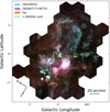 |
Fig. 1 Galactic center, as seen combining optical ionized gas and radio continuum emission. 1.284 GHz radio continuum emission imaged by MeerKAT (green; Heywood et al. 2022) fills the plane, with narrow filaments extending vertically. LVM cannot directly probe the heavily extincted midplane, but bright line emission is apparent above and below, showing a variety of emission line ratios as traced by Hα (orange), [S II] (pink) and [S III] (blue). Clearly this field produces projections of many objects blended along this complicated line-of-sight. For annotation and labeling of the GCL, see Figure 2. |
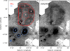 |
Fig. 2 [S III] suffers least from extinction, and provides the most complete and accurate view of the morphology of ionized gas in the direction of the Galactic center. The direct view of the GCL (right) traces out clearly the full structure of the lobe, as annotated and divided into subregions (left). The “Integrated” full lobe (solid red line) has further been subdivided into components (dashed red lines) labeled GCL-1 to GCL-5, along with a single smaller region directly in the center (GCL-C). Four bright H II regions (labeled HII-1 to HII-4) are also selected at b<0° (blue lines). GCL-1 and HII-1 to HII-4 have tentative designations as H II regions based on nebulosity in photographic plate surveys (Sharpless 1959; Dubout-Crillon 1976). The Galactic plane is marked with a horizontal dashed gray line. |
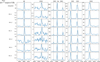 |
Fig. 3 Line emission from the integrated spectra from each GCL subregion shown in Figure 2. Line centers (assuming vLSR=0 km s−1) are marked with vertical dotted lines. |
3 Results
Our analysis of the GCL considers the multiwavelength morphology, characterization of the ionization source, dust extinction, emission line ratio diagnostics, and ionized-gas kinematics.
3.1 Multiwavelength morphology
Literature arguments have been made for associating the GCL with the Galactic center based on its radio continuum morphology, as it can plausibly be seen as a cap or lobe above a chimney leading downward to the Galactic plane. However, from the [S III] map (Figure 2) it is obvious that the radio continuum emission is only part of a larger, closed structure (the ‘Integrated’ GCL, solid red contour). The cap at high Galactic latitudes (b = 1°10′) can be seen to continue smoothly as a bubble structure that forms a complete loop at low Galactic latitudes (b = 0°15′), which in radio continuum is obscured as it is blended in projection with emission from the Galactic plane itself. This geometry naturally complicates interpretation of the region, and by chance the [S III] emission appears to be bright enough to penetrate the dust screen between us and the GCL, but not bright enough that emission from the Galactic center itself is detected. The reported southern cap of the radio continuum emission, extending from the Galactic center toward b = −1°30′ and in good morphological agreement with X-ray emission (Heywood et al. 2019), shows no corresponding [S III] emission (Figure 2. In the context of the [S III] emission, there is no evidence that the GCL is part of a bipolar structure centered on the Galactic plane.
Figure 4 highlights the multiwavelength morphology of the bubble features associated with the GCL. Comparing even Hα with [S III] the completion of the lobe into a bubble was also not apparent due to the heavy extinction at low Galactic latitudes providing an incomplete view of the ionized gas distribution. In comparing these two maps, it is still clear that along specific sightlines, particularly close to GCL-1, there is still significant dust extinction seen in the [S III] images that could hide an ionizing source for the nebula (see Section 4.2 for further discussion).
The MeerKAT radio continuum 1.284 GHz emission (Heywood et al. 2022) traces both thermal and nonthermal sources, and the morphology of the lobe agrees extremely well throughout the various subregions. There is an excess of radio continuum at the edge of the bubble (corresponding to GCL-5), and a deficit toward GCL-1 (where blending with various arcs is pronounced); however, in most respects the morphological agreement is quite striking.
Anderson et al. (2024) pointed out that also the mid-IR emission is consistent with classification of the GCL as an H II region, and we highlight again here that the 8.0μm PAH emission morphology (GLIMPSE; Benjamin et al. 2003, Churchwell et al. 2009) agrees extremely well with the outer edge of the ionized bubble at both edges, and again is simply blended with the plane at the bottom. This alignment is in agreement with the expectation that PAHs are mostly ionized or destroyed close to ionizing sources but glow brightly within the photodisassociation region (PDR), as is commonly seen in Galactic H II regions (Allamandola et al. 1989; Berné et al. 2022). Thermal 24μm dust emission (MIPSGAL; Carey et al. 2009) is also seen associated with this bubble, and overlaps with the particularly highly extincted bottom right edge of the bubble that is faint in the Hα imaging (GCL-5 in Figure 4). This compact dust cloud is cataloged in the literature as AFGL 5376 (Cox & Laureijs 1989; Uchida et al. 1990, 1994).
The 13CO molecular gas, observed as part of the SEDGISM survey (Schuller et al. 2017, 2021), is shown as a 0th moment map that is integrated over the velocity channels from −9.5 to 19.5 km s−1. This is a wider velocity range than was considered in Veena et al. (2023), where they focused on channels from −3.5 to 3.5 that traced the GCL structure; however, the wider velocities also include diffuse molecular gas emission that could represent the approaching and receding sides of the GCL. It remains very challenging to disentangle Galactic plane emission from what may be associated with the GCL at low Galactic latitudes.
The bright subregion GCL-1, identified in archival catalogs as an H II region, also shows an off-center peak in dust emission (both 8.0 and 24 μm), and the suggestion of coincident radio continuum emission (although this region is in a forest of radio filaments and poorly highlighted with the dynamic range shown in Figure 4). It is also coincident with the most prominent 13CO cloud (coincident with GCL-1 and marked in Figure 4 with a dashed red line), with a complicated molecular gas morphology that could be reflecting early stages of stellar feedback carving out bubbles and channels. If this is an H II region in its own right, either distinct or linked to the GCL, then it has a clear blister morphology with the bottom-right edge still heavily embedded while the upper-left side at higher Galactic latitudes can freely expand into the surrounding ISM.
We note that the ionized gas morphology as traced by Hα and [S III] is not entirely what is expected for an H II region, as both show distinctive ring- or shell-like morphologies in the GCL. All the foreground b < 0° H II regions are more compact and centrally concentrated, showing morphologies typical of Galactic H II regions. This hollow structure is particularly unusual for the higher ionization zone of a nebula, traced here by [S III] but in the literature commonly traced by [O III] as these lines are generally concentrated toward the ionizing source (Kewley et al. 2019). However, the ionized gas morphology also necessarily reflects the underlying ISM morphology, so this may simply reflect pre-existing structures present in the ISM in this region. This idea will be discussed in more detail in Section 4.3.
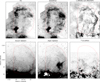 |
Fig. 4 Direct multiwavelength comparison of GCL morphology between LVM optical line emission from Hα and [S III] (top left, center), MeerKAT 1.284 GHz radio continuum (top right), mid-IR dust emission in the PAH dominated 8.0 μm (bottom left) and thermal dust 24 μm (bottom center), and 13CO molecular gas (bottom right). The morphology of the [S III] and radio lobe agrees quite well at high Galactic latitudes, and is encased in an outer shell of PAH emission, with warm dust still in the region interior. CO clouds are offset, outside the GCL boundary. The GCL is marked in a solid red line, and the compact and bright GCL-1 is also marked in a dashed red line. |
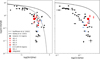 |
Fig. 5 BPT diagnostic diagrams compare the measured [O III]/Hβ with [N I]/Hα and [S II]/Hα for the Integrated GCL and each integrated subregion (red), along with b < 0° H II regions (blue), as labeled in Figure 2. These are compared to a set of Galactic H II regions observed by the DESIRED sample (Méndez-Delgado et al. 2023). All regions are consistent with photoionization when compared to the Kewley et al. (2001) demarcation line, and most are also consistent with the empirical Kauffmann et al. (2003) line. |
3.2 Characterizing ionization conditions
In extragalactic studies of ionized nebulae, the determination of whether or not an object is photoionized typically comes from the consideration of multiple emission line ratio diagnostics. Historically, Baldwin et al. (1981) showed that [O III]/Hβ compared to [N II]/Hα provides a robust way to separate photoionized H II regions from planetary nebulae and shocked supernova remnants. Later work included additional diagnostics, primarily [S II]/Hα, to aid in the characterizaiton of the ionizing source. These so-called BPT diagrams are typically divided by demarcation lines determined by theoretical photoionization modeling of integrated H II regions (Kewley et al. 2001), or empirical characterization of integrated galaxies (Kauffmann et al. 2003). The placement of an ionized nebula below these diagnostic demarcations does not guarantee the object is photoionized (Sánchez 2020; Sánchez et al. 2025b), but it commonly used to interpret extralactic observations. These diagnostics are challenging to apply to Galactic sources, as they require an integrated view of the entire nebula to accurately recover emission lines from both the inner and outer ionization zones of the nebula (Kreckel et al. 2024). With its wide-area IFU coverage, LVM is one of the first instruments that can systematically perform this integrated analysis on Galatic H II regions.
In Figure 5 we show these two BPT diagrams for the GCL, including all subregions, and the set of four foreground b<0° H II regions in Figure 2 as representative of typical Galactic H II regions. We require S/N>3 for all lines, resulting in the exclusion of GCL-4, where [O III] is not significantly detected. Note that because all lines are very close in wavelength, no extinction corrections are applied when calculating these line ratios. Even a very high extinction of AV = 4 mag would result in changes to these line ratios well within the error bars. For some context and comparison we overlay data from a set of Galactic H II regions in the DESIRED sample (Méndez-Delgado et al. 2023), but note that these may not recover flux from the entire regions. All regions are consistent with photoionization when compared to the Kewley et al. (2001) demarcation line, and most are also consistent with the empirical Kauffmann et al. (2003) line. In particular, the Integrated and GCL-1 regions are both fully consistent with photoionization, and in good agreement with the DESIRED Galactic H II regions and with the four b < 0° H II regions. From this analysis, any extragalactic study would conclude that the GCL is an H II region.
3.3 Dust reddening and extinction
Due to the high amount of dust extinction evident in this field, comparison of lines with wider wavelength separations and determination of absolute line luminosities is very sensitive to the exact reddening correction applied. Typically this is performed using the Hα/Hβ Balmer decrement, assuming case B recombination, to constrain the normalization of a given extinction or attenuation law; however, these often contain an additional scaling term parameterized by RV. This reflects the steepness of the chosen curve, and the value has been shown to vary significantly from diffuse to dense ISM conditions (Zhang & Green 2025). With the addition of a third hydrogen recombination line, it is possible to also constrain this RV parameter, and ensure even more robust recovery of reddening corrected parameters.
With LVM, at the blue end we cover many additional Balmer lines; however, they are all not detected due to the high dust extinction. Luckily, from the wide wavelength coverage to the red we observe the Paschen 9 recombination line at λ9229 (Pa9). Due to the faintness of this line, we find it is primarily detected within a few individual fibers that contain the brightest regions of the GCL, and within the high surface brightness GCL-1 region. In Figure 6 we compare Pa9/Hα to Hα/Hβ for all individual fibers with S/N>5 (gray) and S/N>10 (red). As most extinction laws are very similar in shape in the optical, we adopt the Fitzpatrick (1999) extinction curve and overplot lines for fiducial values of RV=3.1 (dashed, typical of diffuse conditions; Cardelli et al. 1989) and RV=4.05 (dotted, typical of denser conditions; Calzetti et al. 2000). We find our high confidence detections and the GCL-1 region fall between these two regimes, consistent with RV=3.6, and adopt this value for the remainder of our analysis. This is typical for translucent regions in the ISM, and may be associated with changes in the dust size distribution (Zhang et al. 2025). In addition, we note that this is significantly different from the value of RV=2 that has previously been determined for the Galactic center (Popowski 2000; Nishiyama et al. 2008), providing additional evidence for more local, star-forming ISM conditions in the GCL.
Adopting this fixed value of RV=3.6, we used pyneb (Luridiana et al. 2012) to convert our Hα/Hβ line ratios to a measurement of the reddening, E(B-V), in each integrated region. We find values ranging between 0.5 and 1.5 mag, with most at ~1.2 mag (AV = 4.3 mag), in very good agreement with estimates from broadband colors in the direction of the GCL (Tsuboi et al. 2020).
3.4 Oxygen abundance diagnostics
One of the confusing aspects of the GCL is its low reported value of Te~3500 K based on radio recombination line measurements (Law et al. 2009; Anderson et al. 2024). Unfortunately, we are unable to detect any of the faint auroral lines (e.g., [N II]λ5755, [S II]λ6312, [O II]λλ7320,7330) that would allow us to directly measure Te. From the [S II]λ6717/[S II]λ6731 density diagnostic we are also unable to provide strong constraints on the electron density, ne, with all measurements consistent with the low-density limit (ne < 100 cm−3) within the uncertainties. Instead, we consider our strong-line ratios that are sensitive to changes in Te and metallicity (Kewley et al. 2019), within the context of the DESIRED sample of Galactic H II regions.
Figure 7 shows Te([N II]) as a function of [N II]/[S II] and [N II]/Hα for a sample of ~40 Galactic H II regions, colored by their Galactocentric radius (RG). Here, the distances are taken from Méndez-Delgado et al. (2022), and based on the identification of ionizing stellar sources from Gaia that have robust parallax measurements. Each line ratio shows a correlation with Te, which we highlight by carrying out a linear fit to all objects with RG < 8.5 kpc (interior to the solar radius). We mark the values for the Integrated GCL (solid red line) and GCL-1 (dashed red line), which are slightly offset from each other but would both overlap with the sample of Galactic H II regions. These line ratios correspond to Te~7000–8000 K, although we emphasize that there is also significant scatter (~1000 K) in the Galactic H II regions at fixed line ratios, making this a weak diagnostic of Te. Te~7000–8000 K is slightly lower than the value typically associated with solar radius from the Orion Nebula (8300 K; Méndez-Delgado et al. 2022), but significantly higher than the value reported from radio recombination lines.
As Te is typically of interest as a diagnostic of the gas-phase metallicity, 12+log(O/H), with lower Te corresponding to higher 12+log(O/H) due to more efficient metal cooling, we also consider the metallicity of each region using integrated strongline abundances. From our constraints on the dust reddening (Section 3.3), we correct all detected lines for extinction and calculate the metallicity using prescriptions that focus on only the red part of the spectrum. We are able to apply the Pilyugin & Grebel (2016) S calibration and the N2S2 Dopita et al. (2016) calibration to both the Integrated GCL and GCL-1. These two calibrations are generally well correlated (Groves et al. 2023); however, the N2S2 prescription is typically 0.2 dex higher than the S calibration, partly because of the different zero-points (S calibration and N2S2 adopt different solar values of 12 + log(O/H) = 8.69 and 8.77, from Asplund et al. 2021 and Nieva & Przybilla 2012, respectively). For the Ingegrated GCL (GCL-1) we find a value of 12+log(O/H) from N2S2 of 8.67±0.03 (8.93 ± 0.01), and from the S calibration we find a value of 8.50±0.03 (8.63±0.01). We discuss the implications of our Te and metallicity measurements on the distance to the GCL in Section 4.1.
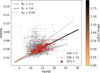 |
Fig. 6 Comparison of Pa9/Hα/ with Hα/Hβ to place constraints on the shape of the dust extinction law. Individual fibers with modest (S/N>5; gray) and high (S/N>10; red) confidence detections of Pa9, along with the integrated measurement from GCL-1, are compared with predictions from the Fitzpatrick (1999) extinction curve with a range of RV values (dotted, dashed, and solid lines). The solid line is further colored to show how the lines ratios would vary with changes in E(B-V). We find that RV=3.6 gives the best agreement, and corresponds to values of E(B-V) = 1.0–1.5. |
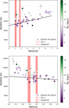 |
Fig. 7 Te [N II] as a function of [N II]/[S II] (top) and [N II]/[S II] (bottom) for a sample of Galactic H II regions (Méndez-Delgado et al. 2023). Points are colored by their Galactocentric radius (RG), and to guide the eye a linear fit (black) is performed for regions within the solar radius (RG < 8.5 kpc). Our Integrated GCL (solid red line) and GCL-1 (dashed red line) measurements are in agreement with the Galactic H II regions, and consistent with a Te ~ 7000–8000 K. |
3.5 Kinematics
Figure 8 shows the ionized gas kinematics across our field, as measured from the [N II] line, and highlights the narrow range of velocities (vLSR ~ −5 to 5 km s−1) across the GCL. We see no obvious signs of expansion, or gradients in Galactic longitude (which might be associated with Galactic rotation at the Galactic center), in good agreement with what has been previously reported from the RRL kinematics (Nagoshi et al. 2019). These kinematics are also in rough agreement with what is reported from the 13CO line (Veena et al. 2023). The measured intrinsic velocity dispersion measured in the shell, as constrained by [N II] and corrected for the instrumental line spread function, is typical for H II regions (10–15 km s−1). We see no prominent indications of further line broadening that could be measured at our S/N and spectral resolution.
We also note that the complex of bright line emission at b < 0°, including the four H II regions isolated in Figure 2, span a very narrow range of velocities and is offset to higher velocities (vLSR ~ 10–15 km s−1). This suggests that this complex is at a slightly different distance than the GCL, but also not at the Galactic center (as there are no Galactic rotation signatures).
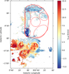 |
Fig. 8 Map of the ionized gas velocity based on the [N II] line centroid, which is masked at S/N<20. The GCL (red line) shows a uniform velocity structure, which is offset from the b < 0° H II regions (blue lines). |
4 Discussion
Taking into account our new constraints on the optical emission line characteristics of the GCL, we reconsider what, and where, this object is.
4.1 Determining the distance to the GCL
While the morphology and geometry of the GCL has long led to the assumption that it is associated with an outflow located at a distance of ~8.5 kpc in the Galactic center (Bland-Hawthorn & Cohen 2003), recent work has convincingly argued that it is instead a foreground H II region (Nagoshi et al. 2019; Tsuboi et al. 2020; Anderson et al. 2024; Hurley-Walker et al. 2024). Based on the optical emission line diagnostics we confirm that the GCL is photoionized, and consistent with other Galactic H II regions.
The development of new 3D dust mapping of the Milky Way has provided a remarkable new way to understand the ISM structures in absolute distance units, without the uncertainties associated with degenerate kinematic constraints. Particularly along the line of sight directly toward the Galactic center, this offers a completely new opportunity to constrain the physical location of the GCL. In Figure 9 we compare our reddening measurements (E(B-V); in red) from the Hα/Hβ Balmer decrement in each integrated region with the integrated reddening as a function of distance along that specific line of sight, as measured in two of the recent 3D dust maps and accessed with the python package dustmaps (Green 2018). The DECaPS map from Zucker et al. (2025) provides the most suitable comparison (orange), as it focuses on the southern Galactic plane using a combination of optical and infrared stellar catalogs to constrain the dust distribution out to maximum distances of 10 kpc. We also include constraints from the Edenhofer et al. (2024) dust map (blue), which is determined using the Gaia BP/RP spectra, but is only available out to distances of 2 kpc. For context, we include measurements toward individual Gaia stars (gray points), as determined from the Gaia BP/RP spectra (Zhang et al. 2023), which are within 9′ of the region center.
Strikingly, the reddening measured from the ionized gas along all sightlines is consistent with a distance of ~2 kpc, particularly when compared to the DECaPS maps. In all tracers, it is clear that there is a sheet of dust at ~1 kpc, causing a jump in the reddening, but what emerges in the DECaPS maps is a second sheet at ~2 kpc that causes any more distant emission to suffer extremely high E(B-V)>2 reddening. This is particularly pronounced along certain sightlines (e.g., GCL-C, and GCL-2, −4 and −5). GCL-1 appears to exhibit slightly higher E(B-V) than would be predicted from the dust maps; however, from the multiwavelength imaging (Figure 4) it is clear that there is a localized dust concentration associated with this region that could be expected to produce locally elevated E(B-V). From these dust constraints, it is clear that the GCL cannot be at the Galactic center, and must be at a distance of at most 2 kpc from the sun.
While our measurements of Te and 12+log(O/H) are not as precise as E(B-V), these can also provide rough constraints on the radial location of the GCL given the established temperature and metallicity gradients in the Milky Way. In Figure 10 we show the distribution of the optically determined Te[N II] as a function of distance for the DESIRED H II regions (also shown in Figure 7), along with the Te determined from radio recombination line observations (Wenger et al. 2019). The alternate y axis shows a conversion of Te to 12+log(O/H) using the relation determined by Martínez-Hernández et al. (2026), assuming the presence of temperature fluctuations (t2 > 0). Our estimation of Te~7000–8000 K, based on the emission line ratios presented in Section 3.4, is consistent with RG=4–10 kpc (distances of 0–4 kpc), although we note that this Te is physically inconsistent with the observed narrow radio recombination line profiles (Law et al. 2009; Anderson et al. 2024). However, Te~7000–8000 K is also in very rough agreement with the strongline metallicities (ranging from 8.5 to 8.8) that are inferred, with large uncertainties introduced depending on the metallicity prescription and region considered. While there are limited measurements available at distances beyond 4 kpc, again our constraints strongly rule out a location directly at the Galactic center.
4.2 Which ionizing stars might be associated with the GCL
One piece of the puzzle that is still missing is the robust identification of an ionizing source for this nebula. Anderson et al. (2024) suggested various candidates, particularly in regions close to the 24 μm bright dust feature, but none of them have a firm classification as an O type star. Based on our extinction corrected Hα flux, and assuming a distance of 2 kpc (see Section 4.1), we recover a total Hα luminosity (accounting for the 83% filling factor) for the GCL Integrated region of 1.5×1037 erg s−1. Given its ~35 pc diameter size, this suggest that the GCL also approximately follows the H II region size-luminosity relation, as measured in extragalactic systems (Barnes et al. 2026). If we were to consider GCL-1 alone as an H II region, as it is reported in the literature photometric nebular catalogs as RCW 138, then it has a total Hα luminosity of 3.9 × 1036 erg s−1. These luminosities are consistent with the ionizing photon flux expected from an individual O 5.5 V star (log Q0 = 49.1; Martins et al. 2005), or at least 10 B type stars (Sternberg et al. 2003).
Most literature catalogs of massive stars do not cover this part of the sky (Clark et al. 2021; Pantaleoni González et al. 2025). In a renewed effort to search for O and B type stars that could be ionizing the GCL, we consider a recent catalog of OB stars (Zari et al. 2021) and select all objects where the distance (as inferred from the parallax) is between 1.5 and 2.5 kpc. A subset of these (in color) have additional characterization of the stellar parameters (log g, log Teff) available based on SDSS-V Milky Way Mapper (MWM) spectroscopy (BOSSNet; Sizemore et al. 2024). Figure 11 shows their location with respect to the GCL, colored by their distance (right) and when available also their reddening (E(B-V), center) and effective temperature (Teff, right). None of them are characterized as O type stars (which would require log Teff > 4.5), and there is no apparent concentration or cluster in the center of the lobe. A single star, Gaia DR3 4060180404854339328, is located slightly more central to the GCL, with E(B-V)~0.8 mag, consistent with what is obtained from the Balmer decrement; however, with only Teff~12 000 K it would seem like a B type star that is insufficient to power this entire nebula. Interestingly, there is a suggestion that these OB stars are instead clustered around the outer ring of the GCL. This is even more apparent when including all OB stars with distances between 0 and 3 kpc (black crosses), as they strongly avoid the location directly at the center of the GCL.
An interesting potential candidate for the ionization source of the lobe is the cluster associated with GCL-1, [DB2000] 58. In Kharchenko et al. (2013), isochrone fitting of this young open cluster resulted in an age of ~1 Myr, and there are clearly B stars identified by Zari et al. (2021) associated with it. While the distance estimate of 1 kpc is slightly closer than what we infer, the cluster is clearly heavily embedded, with E(B-V) = 1.978 mag, which is one of the highest reddenings reported in that work and may result in a distance bias. However, the location of this cluster and of GCL-1 is clearly off-center from the GCL and located instead on the edge, making the interpretation of the geometry challenging.
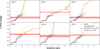 |
Fig. 9 E(B-V) reddening as a function of distance toward each of our regions (see Figure 2), comparing measurements from stars and from gas. Our measurements from the Balmer decrement (red) integrated across each subregion are compared with 3D dust maps derived from stars (orange, Zucker et al. 2025; blue, Edenhofer et al. 2024), and constrain the distance of the GCL to ~2 kpc. The widths of each line indicate the 1σ uncertainties. We also show reddening along sightlines to individual Gaia sources (gray points). |
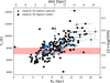 |
Fig. 10 Te as a function of Galactocentric radius (RG), for a sample of optical [N II] (blue, Méndez-Delgado et al. 2023) and radio recombination (black, Wenger et al. 2019) line observations of H II regions. The alternate y axis converts these Te measurements to a metallicity constraint by adopting the prescription that assumes the presence of temperature fluctuations (Martínez-Hernández et al. 2026). Our constraint for the GCL (red band) places it at a distance of less than 4 kpc. |
4.3 A possible counterpart to Barnard’s Loop
The unusual [S III] morphology, which is not concentrated on a ionizing source but instead forms a ring or shell, is reminiscent of what is seen in the nearby structure surrounding the Orion Nebula on large scales, known as Barnard’s Loop (Barnard 1894). Extending over 10° in diameter in the sky, Figure 12 demonstrates that the [S III] morphology observed by the LVM of Barnard’s Loop is strikingly similar to the GCL. While bright in Hα and [S III] it is faint in [O III], and is thought to be mainly photoionized by the massive stars located in the Orion Nebula (M 42), although it does not sit directly in the center of the loop. Recent work has shown it is actually a closed bubble (Ochsendorf et al. 2015), possibly associated with a recent (<1 Myr) supernova event. In a 3D kinematic study of the dust and stars associated with the region, Foley et al. (2023) showed that Barnard’s Loop corresponds to a large dust cavity, and again assert that it has been carved out by past supernovae events. Interestingly, like the GCL (Law et al. 2009; Anderson et al. 2024) it also has a low reported value of Te~5200 K from radio recombination line measurements (Gaylard 1984) and Te~6000 K from a combination of Hα and radio continuum (Heiles et al. 2000), which is ~2300 K lower than what is reported for the Orion Nebula itself (Méndez-Delgado et al. 2022).
An examination of optical line ratio diagnostics in the LVM coverage of Barnard’s Loop, compared to the H II region at the young embedded Flame Nebula (Kreckel et al. 2024), is similar to what is seen in a comparison between the GCL and GCL-1. Using a single LVM tile (tileid=1029104) that is centered on a part of Barnard’s Loop at (ra,dec) = (86.80012 deg, 1.28296 deg), we find that the ionized gas ring exhibits very low reddening (E(B-V)=0.02 mag) compared to the dust-enshrouded Flame Nebula (E(B-V)=0.54 mag). Both the GCL and Barnard’s Loop have low extinction corrected [S III]/[S II] line ratios of ~0.2–0.3, significantly lower than the ratio of ~0.9 that is measured in the Flame Nebula. As [S III]/[S II] is a proxy for changes in ionization parameter, reflecting the number of ionizing photons impacting the gas, this is also suggestive that the GCL be removed by some significant distance from the primary ionization source, as in Barnard’s Loop. [S II]/Hα is also similar in both structures, further confirming the similarities in the ionization state of the gas in both shells.
If the GCL is at a distance of 2 kpc, then its angular size corresponds to a physical diameter of ~35 pc. This is about half the size of Barnard’s Loop. While we do not directly constrain an expansion velocity for the GCL due to the limited spectral resolution of the LVM, we do measure a ~10 km s−1 velocity gradient from top to bottom. This is similar to tentative broadening seen in the GCL center in radio recombination line observations from Law et al. (2009), in both the center of their ![Mathematical equation: $\[\mathrm{b}\text{=0}^\circ_\cdot45\]$](/articles/aa/full_html/2026/06/aa59505-26/aa59505-26-eq1.png) strip and the edge of their GCL4 strip. Intriguingly, this signature is also seen in the 13CO SEDGISM data (Figure 13), and we model the position-velocity diagram along b = 0°24′ as a blister as
strip and the edge of their GCL4 strip. Intriguingly, this signature is also seen in the 13CO SEDGISM data (Figure 13), and we model the position-velocity diagram along b = 0°24′ as a blister as
![Mathematical equation: $\[v(x)=v_{\mathrm{sys}}+v_{\exp } \sqrt{1-\left(\frac{\Delta \theta}{\theta_R}\right)^2}.\]$](/articles/aa/full_html/2026/06/aa59505-26/aa59505-26-eq2.png) (1)
(1)
With θR the angular radius of the bubble and and Δθ the angular separation from the center (ℓ0 = 359°39′0″, b0 = 0°24′0″). The fit yields an expansion velocity of vexp = 12.5 km s−1, comparable to that measured in Barnard’s Loop (Reynolds & Ogden 1979). Using the solution of Weaver et al. (1977) the bubble expansion age can be estimated to be ~0.7 Myr. Given its redshifted velocity this blister is expanding away from us, downstream to the spiral arm, similar to what is seen in nearby galaxies (Watkins et al. 2023). With this small estimated age but accumulation of molecular material, is likely this bubble originated from supernovae feedback (as in the case of Barnard’s Loop), and the association of cataloged OB stars with the rim of the GCL is suggestive of propagated star formation following shell compression driven in a past supernova event. However, it is unlikely to be associated with the very young (1 Myr) cluster currently at GCL-1.
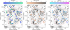 |
Fig. 11 Locations of OB stars from Zari et al. (2021) compared to the morphology of the GCL (grayscale, traced here by [S III]). Stars with parallax distances between 1.5 and 2.5 kpc are colored by their distance (left), reddening (E(B-V), center) and effective temperature (Teff, right). All stars with distances between 0-3 kpc are also shown in black (crosses). Interestingly, most stars avoid the center of the GCL, and none are characterized as O type (log Teff > 4.5). |
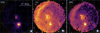 |
Fig. 12 Barnard’s Loop in LVM: [O III] (left), Hα (center), [S III] (right). Covering nearly 15° × 15° across the sky (~100 pc in diameter), this ionized ring is associated with the O type stars powering M 42, NGC 2024 and IC434 (Kreckel et al. 2024). |
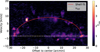 |
Fig. 13 Position-velocity slice across the GCL center at b = 0°24′ in the 13CO SEDGISM data, as modeled by a simple expanding blister shell (Equation (1)). |
5 Conclusions
We present a new SDSS-V LVM optical IFU map covering 1.5 × 3 deg in the direction of the Galactic center, covering the so-called “Galactic center lobe” (GCL). We confirm recent results that identify this as a foreground object (Nagoshi et al. 2019; Tsuboi et al. 2020; Hurley-Walker et al. 2024; Anderson et al. 2024), and not associated with the Galactic center. To this end, we suggest the acronym GCL be repurposed to instead abbreviate the name “greatly confused loop”.
In our work, we leverage new optical emission line constraints on the GCL to provide concrete answers to where, and what, the GCL is.
Using [S III]λ9532 emission line maps, which suffers the least extinction, we identify ionized gas emission throughout a full, closed outer loop, and further note that this high ionization ion does does not fill the bubble interior. There is a very good morphological correspondence between the diffuse radio continuum emission, and 8.0 μm PAH dust emission.
All optical line diagnostics that we consider are consistent with photoionization. The lobe is bright in Hα, [S III], [S II] and [N II]. While detected in integrated spectra across the GCL, [O III] is not strongly detected in resolved maps.
Using Pa9/Hα and Hα/Hβ we constrain RV=3.6 and infer a dust reddening of E(B-V)=1.0 to 1.5 mag. Combined with 3D dust maps, this directly constrains the distance to the GCL to ~2 kpc.
We estimate Te [N II]=7000–8000 K based on strongline ratios, when compared to a sample of Galactic H II regions, which implies slightly super-solar metallicity, and is strongly discrepant from the radio recombination line Te=3.500 K. Based on the Galactic radial Te gradient, this implies a distance of less than 4 kpc.
[N II] line kinematics show a uniform velocity structure across the GCL, further confirming that the entire bubble is one associated structure.
Given the ~2 kpc distance of this photoionized structure, the size and emission line morphology is strongly reminiscent of what is seen in the nearby Barnard’s Loop. It may indicate a similar origin, of a past supernova event clearing a cavity 35 pc in diameter, which is currently the site of new OB star formation and enables radiation to propagate through the cavity interior to sustain the photoionization of the shell. The young blister-like (~1 Myr) cluster associated with GCL-1/RCW 138 may play a significant role in the photoionization of the GCL structure.
Given the available multiwavelength views of this region, we have shown that the specific dust extinction structure along this line of sight results in the ionized gas unveiling most accurately the closed, bubble-like morphology of the GCL, as everything more distant is completely extincted. Mid-IR PAH features and radio continuum emission are blended, which has obstructed the identification of this feature in past work. Parallels with Galactic center X-ray features, and the base of the Fermi bubble, must be largely coincidental.
Data availability
Following SDSS data access policies, all reduced data and data analysis pipeline products will be made publicly available in an upcoming SDSS public data release to be hosted and searchable on the SDSS SkyServer (https://skyserver.sdss.org/) and Science Archive Server (SAS; https://data.sdss.org/sas/).
Acknowledgements
We thank the referee for their careful reading, which helped to improve the clarity and quality of this work. Many thanks to Ian Heywood for providing the MeerKAT data over a larger field of view. K.K. gratefully acknowledges funding from the Deutsche Forschungsgemeinschaft (DFG, German Research Foundation) in the form of an Emmy Noether Research Group (grant number KR4598/2-1, PI: Kreckel) and the European Research Council’s starting grant ERC StG-101077573 (“ISM-METALS”). K.K. and S.K. acknowledge funding by the Deutsche Forschungsgemeinschaft (DFG, German Research Foundation) – Project number 558818801. O.E. acknowledges funding from the Deutsche Forschungsgemeinschaft (DFG, German Research Foundation) – project-ID 541068876. J.G.F-T gratefully acknowledges the grants support provided by ANID Fondecyt Postdoc No. 3230001 (Sponsoring researcher), the Joint Committee ESO-Government of Chile under the agreement 2023 ORP 062/2023, and the support of the Doctoral Program in Artificial Intelligence, DISC-UCN. J.E.M.-D. and R.de.J.Z. thank the support by SECIHTI CBF-2025-I-2048 project “Resolviendo la Física Interna de las Galaxias: De las Escalas Locales a la Estructura Global con el SDSS-V Local Volume Mapper” (PI: Méndez-Delgado). J.E.M.-D. and R.de.J.Z. thank the support by UNAM/DGAPA/PAPIIT/IA103326 project “DESIRED (DEep Spectra of Ionized Regions Database): de las emisiones más sutiles a la física fundamental del universo” (PI: Méndez-Delgado). S.F.S. acknowledges the support by CBF-2025-I-236 project granted by the Secretaría de Ciencia, Humanidades, Tecnología e Innovación (SECIHTI) of the Mexican Federal Government, and the PID2022-136598NB-C31 (ESTALLIDOS) grant by the Spanish Ministery of Science and Innovation (MCINN). A.Z.L.A. gratefully acknowledges the support provided by the Post-doctoral Program (POSDOC) of UNAM (Universidad Nacional Autónoma de México). Funding for the Sloan Digital Sky Survey V has been provided by the Alfred P. Sloan Foundation, the Heising-Simons Foundation, the National Science Foundation, and the Participating Institutions. SDSS acknowledges support and resources from the Center for High-Performance Computing at the University of Utah. SDSS telescopes are located at Apache Point Observatory, funded by the Astrophysical Research Consortium and operated by New Mexico State University, and at Las Campanas Observatory, operated by the Carnegie Institution for Science. The SDSS web site is www.sdss.org. SDSS is managed by the Astrophysical Research Consortium for the Participating Institutions of the SDSS Collaboration, including the Carnegie Institution for Science, Chilean National Time Allocation Committee (CNTAC) ratified researchers, Caltech, the Gotham Participation Group, Harvard University, Heidelberg University, The Flatiron Institute, The Johns Hopkins University, L’Ecole polytechnique fédérale de Lausanne (EPFL), Leibniz-Institut für Astrophysik Potsdam (AIP), Max-Planck-Institut für Astronomie (MPIA Heidelberg), Max-Planck-Institut für Extraterrestrische Physik (MPE), Nanjing University, National Astronomical Observatories of China (NAOC), New Mexico State University, The Ohio State University, Pennsylvania State University, Smithsonian Astrophysical Observatory, Space Telescope Science Institute (STScI), the Stellar Astrophysics Participation Group, Universidad Nacional Autónoma de México, University of Arizona, University of Colorado Boulder, University of Illinois at Urbana-Champaign, University of Toronto, University of Utah, University of Virginia, Yale University, and Yunnan University. This work made use of the Cube Analysis and Rendering Tool for Astronomy (CARTA; Comrie et al. 2021), and a number of python packages, namely the main ASTROPY package (Astropy Collaboration 2013, 2018, 2022), NUMPY (Harris et al. 2020), MATPLOTLIB (Hunter 2007) and SPECTRAL-CUBE3.
References
- Allamandola, L. J., Tielens, A. G. G. M., & Barker, J. R. 1989, ApJS, 71, 733 [Google Scholar]
- Anderson, L. D., Bania, T. M., Balser, D. S., et al. 2014, ApJS, 212, 1 [Google Scholar]
- Anderson, L. D., Armentrout, W. P., Johnstone, B. M., et al. 2015, ApJS, 221, 26 [NASA ADS] [CrossRef] [Google Scholar]
- Anderson, L. D., Luisi, M., Liu, B., et al. 2024, ApJ, 969, 43 [Google Scholar]
- Asplund, M., Amarsi, A. M., & Grevesse, N. 2021, A&A, 53, A141 [Google Scholar]
- Astropy Collaboration (Robitaille, T. P., et al.) 2013, A&A, 558, A33 [NASA ADS] [CrossRef] [EDP Sciences] [Google Scholar]
- Astropy Collaboration (Price-Whelan, A. M., et al.) 2018, AJ, 156, 123 [Google Scholar]
- Astropy Collaboration (Price-Whelan, A. M., et al.) 2022, ApJ, 935, 167 [NASA ADS] [CrossRef] [Google Scholar]
- Avedisova, V. S., & Palous, J. 1989, Bull. Astron. Inst. Czechoslovakia, 40, 42 [Google Scholar]
- Baldwin, J. A., Phillips, M. M., & Terlevich, R. 1981, PASP, 93, 5 [Google Scholar]
- Barnard, E. E. 1894, Popular Astron., 2, 151 [Google Scholar]
- Barnes, A. T., Chandar, R., Kreckel, K., et al. 2026, A&A, 706, A95 [NASA ADS] [CrossRef] [EDP Sciences] [Google Scholar]
- Benjamin, R. A., Churchwell, E., Babler, B. L., et al. 2003, PASP, 115, 953 [Google Scholar]
- Berné, O., Habart, É., Peeters, E., et al. 2022, PASP, 134, 054301 [CrossRef] [Google Scholar]
- Bland-Hawthorn, J., & Cohen, M. 2003, ApJ, 582, 246 [Google Scholar]
- Brogan, C. L., Nord, M., Kassim, N., Lazio, J., & Anantharamaiah, K. 2003, Astron. Nachr. Suppl., 324, 17 [Google Scholar]
- Calzetti, D., Armus, L., Bohlin, R. C., et al. 2000, ApJ, 533, 682 [NASA ADS] [CrossRef] [Google Scholar]
- Cardelli, J. A., Clayton, G. C., & Mathis, J. S. 1989, ApJ, 345, 245 [Google Scholar]
- Carey, S. J., Noriega-Crespo, A., Mizuno, D. R., et al. 2009, PASP, 121, 76 [Google Scholar]
- Churchwell, E., Babler, B. L., Meade, M. R., et al. 2009, PASP, 121, 213 [Google Scholar]
- Clark, J. S., Patrick, L. R., Najarro, F., Evans, C. J., & Lohr, M. 2021, A&A, 49, A43 [Google Scholar]
- Comrie, A., Wang, K.-S., Hsu, S.-C., et al. 2021, Astrophysics Source Code Library [record ascl:2103.031] [Google Scholar]
- Cox, P., & Laureijs, R. 1989, IAU Symp., 136, 121 [Google Scholar]
- Dopita, M. A., Kewley, L. J., Sutherland, R. S., & Nicholls, D. C. 2016, Ap&SS, 361, 61 [NASA ADS] [CrossRef] [Google Scholar]
- Drory, N., Blanc, G. A., Kreckel, K., et al. 2024, AJ, 168, 198 [NASA ADS] [CrossRef] [Google Scholar]
- Dubout-Crillon, R. 1976, A&AS, 25, 25 [Google Scholar]
- Dutra, C. M., & Bica, E. 2000, A&A, 359, L9 [Google Scholar]
- Edenhofer, G., Zucker, C., Frank, P., et al. 2024, A&A, 685, A82 [NASA ADS] [CrossRef] [EDP Sciences] [Google Scholar]
- Fitzpatrick, E. L. 1999, PASP, 111, 63 [Google Scholar]
- Foley, M. M., Goodman, A., Zucker, C., et al. 2023, ApJ, 947, 66 [NASA ADS] [CrossRef] [Google Scholar]
- Gaylard, M. J. 1984, MNRAS, 211, 149 [Google Scholar]
- Green, G. 2018, J. Open Source Softw., 3, 695 [NASA ADS] [CrossRef] [Google Scholar]
- Groves, B., Kreckel, K., Santoro, F., et al. 2023, MNRAS, 520, 4902 [Google Scholar]
- Harris, C. R., Millman, K. J., van der Walt, S. J., et al. 2020, Nature, 585, 357 [NASA ADS] [CrossRef] [Google Scholar]
- Heiles, C., Haffner, L. M., Reynolds, R. J., & Tufte, S. L. 2000, ApJ, 536, 335 [NASA ADS] [CrossRef] [Google Scholar]
- Henshaw, J. D., Barnes, A. T., Battersby, C., et al. 2023, ASP Conf. Ser., 534, 83 [NASA ADS] [Google Scholar]
- Herbst, T. M., Bizenberger, P., Blanc, G. A., et al. 2024, AJ, 168, 267 [Google Scholar]
- Heyvaerts, J., Norman, C., & Pudritz, R. E. 1988, ApJ, 330, 718 [Google Scholar]
- Heywood, I., Camilo, F., Cotton, W. D., et al. 2019, Nature, 573, 235 [Google Scholar]
- Heywood, I., Rammala, I., Camilo, F., et al. 2022, ApJ, 925, 165 [NASA ADS] [CrossRef] [Google Scholar]
- Hilder, T., Casey, A. R., Dalcanton, J. J., et al. 2026, ApJ, 997, 339 [Google Scholar]
- Hunter, J. D. 2007, Comp. Sci. Eng., 9, 90 [NASA ADS] [CrossRef] [Google Scholar]
- Hurley-Walker, N., Anderson, L. D., Luisi, M., et al. 2024, ApJ, 969, 42 [Google Scholar]
- Kassim, N. E., Larosa, T. N., & Erickson, W. C. 1986, Nature, 322, 522 [Google Scholar]
- Kauffmann, G., Heckman, T. M., Tremonti, C., et al. 2003, MNRAS, 346, 1055 [Google Scholar]
- Kewley, L. J., Dopita, M. A., Sutherland, R. S., Heisler, C. A., & Trevena, J. 2001, ApJ, 556, 121 [Google Scholar]
- Kewley, L. J., Nicholls, D. C., & Sutherland, R. S. 2019, ARA&A, 57, 511 [Google Scholar]
- Kharchenko, N. V., Piskunov, A. E., Schilbach, E., Röser, S., & Scholz, R.-D. 2013, A&A, 558, A53 [NASA ADS] [CrossRef] [EDP Sciences] [Google Scholar]
- Kollmeier, J. A., Rix, H.-W., Aerts, C., et al. 2026, AJ, 171, 52 [Google Scholar]
- Konidaris, N. P., Herbst, T., Froning, C., et al. 2024, SPIE Conf. Ser., 13096, 130961Z [Google Scholar]
- Kreckel, K., Egorov, O. V., Egorova, E., et al. 2024, A&A, 689, A352 [NASA ADS] [CrossRef] [EDP Sciences] [Google Scholar]
- Law, C. J. 2010, ApJ, 708, 474 [Google Scholar]
- Law, C. J., Backer, D., Yusef-Zadeh, F., & Maddalena, R. 2009, ApJ, 695, 1070 [NASA ADS] [CrossRef] [Google Scholar]
- Luridiana, V., Morisset, C., & Shaw, R. A. 2012, IAU Symp., 283, 422 [NASA ADS] [Google Scholar]
- Martínez-Hernández, I. R., Méndez-Delgado, J. E., Esteban, C., et al. 2026, MNRAS, 546, stag 149 [Google Scholar]
- Martins, F., Schaerer, D., & Hillier, D. J. 2005, A&A, 436, 1049 [NASA ADS] [CrossRef] [EDP Sciences] [Google Scholar]
- Méndez-Delgado, J. E., Amayo, A., Arellano-Córdova, K. Z., et al. 2022, MNRAS, 510, 4436 [CrossRef] [Google Scholar]
- Méndez-Delgado, J. E., Esteban, C., García-Rojas, J., et al. 2023, MNRAS, 523, 2952 [CrossRef] [Google Scholar]
- Monteiro, H., & Dias, W. S. 2019, MNRAS, 487, 2385 [Google Scholar]
- Morris, M., & Serabyn, E. 1996, ARA&A, 34, 645 [Google Scholar]
- Nagoshi, H., Kubose, Y., Fujisawa, K., et al. 2019, PASJ, 71, 80 [Google Scholar]
- Nieva, M.-F., & Przybilla, N. 2012, A&A, 539, A143 [NASA ADS] [CrossRef] [EDP Sciences] [Google Scholar]
- Nishiyama, S., Nagata, T., Tamura, M., et al. 2008, ApJ, 680, 1174 [Google Scholar]
- Nossal, S. M., Mierkiewicz, E. J., Roesler, F. L., et al. 2008, J. Geophys. Res. Space Phys., 113, A11307 [Google Scholar]
- Ochsendorf, B. B., Brown, A. G. A., Bally, J., & Tielens, A. G. G. M. 2015, ApJ, 808, 111 [NASA ADS] [CrossRef] [Google Scholar]
- Pantaleoni González, M., Maíz Apellániz, J., Barbá, R. H., et al. 2025, MNRAS, 543, 63 [Google Scholar]
- Parker, E. N. 1966, ApJ, 145, 811 [NASA ADS] [CrossRef] [Google Scholar]
- Pilyugin, L. S., & Grebel, E. K. 2016, MNRAS, 457, 3678 [NASA ADS] [CrossRef] [Google Scholar]
- Ponti, G., Hofmann, F., Churazov, E., et al. 2019, Nature, 567, 347 [Google Scholar]
- Ponti, G., Morris, M. R., Churazov, E., Heywood, I., & Fender, R. P. 2021, A&A, 646, A66 [NASA ADS] [CrossRef] [EDP Sciences] [Google Scholar]
- Popowski, P. 2000, ApJ, 528, L9 [NASA ADS] [CrossRef] [Google Scholar]
- Reich, W., Sofue, Y., & Fuerst, E. 1987, PASJ, 39, 573 [Google Scholar]
- Reynolds, R. J., & Ogden, P. M. 1979, ApJ, 229, 942 [NASA ADS] [CrossRef] [Google Scholar]
- Roeser, S., Demleitner, M., & Schilbach, E. 2010, AJ, 139, 2440 [Google Scholar]
- Sánchez, S. F. 2020, ARA&A, 58, 99 [Google Scholar]
- Sánchez, S. F., Mejía-Narváez, A., Egorov, O. V., et al. 2025a, AJ, 169, 52 [Google Scholar]
- Sánchez, S. F., Muñoz-Tuñón, C., Sánchez Almeida, J., González-Martín, O., & Pérez, E. 2025b, A&A, 704, A145 [NASA ADS] [CrossRef] [EDP Sciences] [Google Scholar]
- Sanchez Sanchez, S. F., Méndez-Delgado, J. E., Mejía-Narváez, A., et al. 2026, Rev. Mexicana Astron. Astrofis., 62, 87 [Google Scholar]
- Sarbadhicary, S. K., Long, K. S., Raymond, J. C., et al. 2026, ApJ, 998, 278 [Google Scholar]
- Sattler, N., Méndez-Delgado, J. E., Kreckel, K., et al. 2026, A&A, 706, A81 [NASA ADS] [CrossRef] [EDP Sciences] [Google Scholar]
- Schenck, D. E., Shirley, Y. L., Reiter, M., & Juneau, S. 2011, AJ, 142, 94 [Google Scholar]
- Schönrich, R., Binney, J., & Dehnen, W. 2010, MNRAS, 403, 1829 [NASA ADS] [CrossRef] [Google Scholar]
- Schuller, F., Csengeri, T., Urquhart, J. S., et al. 2017, A&A, 601, A124 [NASA ADS] [CrossRef] [EDP Sciences] [Google Scholar]
- Schuller, F., Urquhart, J. S., Csengeri, T., et al. 2021, MNRAS, 500, 3064 [Google Scholar]
- Sharpless, S. 1959, ApJS, 4, 257 [Google Scholar]
- Singh, A., Blanc, G. A., Kumari, N., et al. 2026, ApJ, 1001, 238 [Google Scholar]
- Sizemore, L., Llanes, D., Kounkel, M., et al. 2024, AJ, 167, 173 [Google Scholar]
- Skrutskie, M. F., Cutri, R. M., Stiening, R., et al. 2006, AJ, 131, 1163 [NASA ADS] [CrossRef] [Google Scholar]
- Sofue, Y. 1985, PASJ, 37, 697 [Google Scholar]
- Sofue, Y., & Handa, T. 1984, Nature, 310, 568 [Google Scholar]
- Sternberg, A., Hoffmann, T. L., & Pauldrach, A. W. A. 2003, ApJ, 599, 1333 [NASA ADS] [CrossRef] [Google Scholar]
- Tsuboi, M., Tsutsumi, T., Kitamura, Y., et al. 2020, PASJ, 72, L10 [NASA ADS] [CrossRef] [Google Scholar]
- Uchida, Y., Shibata, K., & Sofue, Y. 1985, Nature, 317, 699 [Google Scholar]
- Uchida, K., Morris, M., & Serabyn, E. 1990, ApJ, 351, 443 [Google Scholar]
- Uchida, K. I., Morris, M. R., Serabyn, E., & Bally, J. 1994, ApJ, 421, 505 [Google Scholar]
- Veena, V. S., Riquelme, D., Kim, W.-J., et al. 2023, A&A, 674, L15 [NASA ADS] [CrossRef] [EDP Sciences] [Google Scholar]
- Villa-Durango, M. A., Barrera-Ballesteros, J., Román-Zúñiga, C. G., et al. 2025, MNRAS, 543, 1196 [Google Scholar]
- Wang, Q. D. 2021, MNRAS, 504, 1609 [CrossRef] [Google Scholar]
- Watkins, E. J., Barnes, A. T., Henny, K., et al. 2023, ApJ, 944, L24 [NASA ADS] [CrossRef] [Google Scholar]
- Wayth, R. B., Lenc, E., Bell, M. E., et al. 2015, PASA, 32, e025 [Google Scholar]
- Weaver, R., McCray, R., Castor, J., Shapiro, P., & Moore, R. 1977, ApJ, 218, 377 [Google Scholar]
- Wenger, T. V., Balser, D. S., Anderson, L. D., & Bania, T. M. 2019, ApJ, 887, 114 [NASA ADS] [CrossRef] [Google Scholar]
- Yan, R., Chen, Y., Lazarz, D., et al. 2019, ApJ, 883, 175 [Google Scholar]
- Yusef-Zadeh, F., Morris, M., & Chance, D. 1984, Nature, 310, 557 [NASA ADS] [CrossRef] [Google Scholar]
- Zari, E., Rix, H.-W., Frankel, N., et al. 2021, A&A, 650, A112 [NASA ADS] [CrossRef] [EDP Sciences] [Google Scholar]
- Zhang, X., & Green, G. M. 2025, Science, 387, 1209 [Google Scholar]
- Zhang, X., Green, G. M., & Rix, H.-W. 2023, MNRAS, 524, 1855 [NASA ADS] [CrossRef] [Google Scholar]
- Zhang, X., Hensley, B. S., & Green, G. M. 2025, ApJ, 979, L17 [Google Scholar]
- Zucker, C., Saydjari, A. K., Speagle, J. S., et al. 2025, ApJ, 992, 39 [Google Scholar]
Appendix A Further details on the low Galactic latitude HII regions
In Figure A.1 we show spectral features of key emission lines, as detected in the integrated spectra of four H II regions at b<0° (see Figure 2).
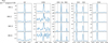 |
Fig. A.1 Key spectral features for all four b<0° H II regions labeled in Figure 2. Line centers (assuming vLSR=0 km s−1) are marked with vertical dotted lines. |
A limited amount of information is available for each of these H II regions in the literature; however, they are generally thought to be foreground to the Galactic center region. Cross-identification of these regions with existing catalogs and tentative distance estimates for each are provided. All have been confirmed to be H II regions based on their radio recombination line emission (Anderson et al. 2014, 2015), and are referenced in the WISE Catalog of Galactic HII Regions.
HII-1, which corresponds to Sh 2-16, has an estimated distance of 2.526 ± 0.149 kpc based on the parallax distance to Gaia DR3 4057274876643924096 (LS 4381) of the apparent ionizing source. Its WISE identification is G359.756-00.351.
HII-2, which corresponds to Sh 2-20 and RCW 141, has an estimated distance of 3.909 ± 0.291 kpc (Monteiro & Dias 2019). Its WISE identification is G000.320-00.215.
HII-3, which corresponds to RCW 139, has an estimated distance of 2.41 ± 0.42 kpc based on the Gaia DR3 4057473097944289920 parallax of 0.4148 ± 0.0869 mas for a possible ionizing source. This is consistent with an older distance estimate of 1.7 ± 0.4 kpc (Avedisova & Palous 1989). Its WISE identification is G000.120-00.556.
HII-4, which corresponds to Sh 2-21 and RCW 142, has an estimated distance of 2.0 ± 0.4 kpc (Schenck et al. 2011). Its WISE identification is G000.573-00.855.
These are at a similar (or slightly larger) distance compared to the GCL; however, they have distinctly different kinematics (Figure 8), suggesting that they are not in close physical proximity to the GCL.
All Figures
|
Fig. 1 Galactic center, as seen combining optical ionized gas and radio continuum emission. 1.284 GHz radio continuum emission imaged by MeerKAT (green; Heywood et al. 2022) fills the plane, with narrow filaments extending vertically. LVM cannot directly probe the heavily extincted midplane, but bright line emission is apparent above and below, showing a variety of emission line ratios as traced by Hα (orange), [S II] (pink) and [S III] (blue). Clearly this field produces projections of many objects blended along this complicated line-of-sight. For annotation and labeling of the GCL, see Figure 2. |
| In the text | |
|
Fig. 2 [S III] suffers least from extinction, and provides the most complete and accurate view of the morphology of ionized gas in the direction of the Galactic center. The direct view of the GCL (right) traces out clearly the full structure of the lobe, as annotated and divided into subregions (left). The “Integrated” full lobe (solid red line) has further been subdivided into components (dashed red lines) labeled GCL-1 to GCL-5, along with a single smaller region directly in the center (GCL-C). Four bright H II regions (labeled HII-1 to HII-4) are also selected at b<0° (blue lines). GCL-1 and HII-1 to HII-4 have tentative designations as H II regions based on nebulosity in photographic plate surveys (Sharpless 1959; Dubout-Crillon 1976). The Galactic plane is marked with a horizontal dashed gray line. |
| In the text | |
|
Fig. 3 Line emission from the integrated spectra from each GCL subregion shown in Figure 2. Line centers (assuming vLSR=0 km s−1) are marked with vertical dotted lines. |
| In the text | |
|
Fig. 4 Direct multiwavelength comparison of GCL morphology between LVM optical line emission from Hα and [S III] (top left, center), MeerKAT 1.284 GHz radio continuum (top right), mid-IR dust emission in the PAH dominated 8.0 μm (bottom left) and thermal dust 24 μm (bottom center), and 13CO molecular gas (bottom right). The morphology of the [S III] and radio lobe agrees quite well at high Galactic latitudes, and is encased in an outer shell of PAH emission, with warm dust still in the region interior. CO clouds are offset, outside the GCL boundary. The GCL is marked in a solid red line, and the compact and bright GCL-1 is also marked in a dashed red line. |
| In the text | |
|
Fig. 5 BPT diagnostic diagrams compare the measured [O III]/Hβ with [N I]/Hα and [S II]/Hα for the Integrated GCL and each integrated subregion (red), along with b < 0° H II regions (blue), as labeled in Figure 2. These are compared to a set of Galactic H II regions observed by the DESIRED sample (Méndez-Delgado et al. 2023). All regions are consistent with photoionization when compared to the Kewley et al. (2001) demarcation line, and most are also consistent with the empirical Kauffmann et al. (2003) line. |
| In the text | |
|
Fig. 6 Comparison of Pa9/Hα/ with Hα/Hβ to place constraints on the shape of the dust extinction law. Individual fibers with modest (S/N>5; gray) and high (S/N>10; red) confidence detections of Pa9, along with the integrated measurement from GCL-1, are compared with predictions from the Fitzpatrick (1999) extinction curve with a range of RV values (dotted, dashed, and solid lines). The solid line is further colored to show how the lines ratios would vary with changes in E(B-V). We find that RV=3.6 gives the best agreement, and corresponds to values of E(B-V) = 1.0–1.5. |
| In the text | |
|
Fig. 7 Te [N II] as a function of [N II]/[S II] (top) and [N II]/[S II] (bottom) for a sample of Galactic H II regions (Méndez-Delgado et al. 2023). Points are colored by their Galactocentric radius (RG), and to guide the eye a linear fit (black) is performed for regions within the solar radius (RG < 8.5 kpc). Our Integrated GCL (solid red line) and GCL-1 (dashed red line) measurements are in agreement with the Galactic H II regions, and consistent with a Te ~ 7000–8000 K. |
| In the text | |
|
Fig. 8 Map of the ionized gas velocity based on the [N II] line centroid, which is masked at S/N<20. The GCL (red line) shows a uniform velocity structure, which is offset from the b < 0° H II regions (blue lines). |
| In the text | |
|
Fig. 9 E(B-V) reddening as a function of distance toward each of our regions (see Figure 2), comparing measurements from stars and from gas. Our measurements from the Balmer decrement (red) integrated across each subregion are compared with 3D dust maps derived from stars (orange, Zucker et al. 2025; blue, Edenhofer et al. 2024), and constrain the distance of the GCL to ~2 kpc. The widths of each line indicate the 1σ uncertainties. We also show reddening along sightlines to individual Gaia sources (gray points). |
| In the text | |
|
Fig. 10 Te as a function of Galactocentric radius (RG), for a sample of optical [N II] (blue, Méndez-Delgado et al. 2023) and radio recombination (black, Wenger et al. 2019) line observations of H II regions. The alternate y axis converts these Te measurements to a metallicity constraint by adopting the prescription that assumes the presence of temperature fluctuations (Martínez-Hernández et al. 2026). Our constraint for the GCL (red band) places it at a distance of less than 4 kpc. |
| In the text | |
|
Fig. 11 Locations of OB stars from Zari et al. (2021) compared to the morphology of the GCL (grayscale, traced here by [S III]). Stars with parallax distances between 1.5 and 2.5 kpc are colored by their distance (left), reddening (E(B-V), center) and effective temperature (Teff, right). All stars with distances between 0-3 kpc are also shown in black (crosses). Interestingly, most stars avoid the center of the GCL, and none are characterized as O type (log Teff > 4.5). |
| In the text | |
|
Fig. 12 Barnard’s Loop in LVM: [O III] (left), Hα (center), [S III] (right). Covering nearly 15° × 15° across the sky (~100 pc in diameter), this ionized ring is associated with the O type stars powering M 42, NGC 2024 and IC434 (Kreckel et al. 2024). |
| In the text | |
|
Fig. 13 Position-velocity slice across the GCL center at b = 0°24′ in the 13CO SEDGISM data, as modeled by a simple expanding blister shell (Equation (1)). |
| In the text | |
|
Fig. A.1 Key spectral features for all four b<0° H II regions labeled in Figure 2. Line centers (assuming vLSR=0 km s−1) are marked with vertical dotted lines. |
| In the text | |
Current usage metrics show cumulative count of Article Views (full-text article views including HTML views, PDF and ePub downloads, according to the available data) and Abstracts Views on Vision4Press platform.
Data correspond to usage on the plateform after 2015. The current usage metrics is available 48-96 hours after online publication and is updated daily on week days.
Initial download of the metrics may take a while.