


| Issue |
A&A
Volume 710, June 2026
|
|
|---|---|---|
| Article Number | A264 | |
| Number of page(s) | 15 | |
| Section | Interstellar and circumstellar matter | |
| DOI | https://doi.org/10.1051/0004-6361/202659496 | |
| Published online | 18 June 2026 | |
The Rayleigh–Taylor instability in partially ionised plasmas: Ambipolar diffusion effects in the non-linear phase
1
Laboratoire Univers et Particules de Montpellier (LUPM) Université Montpellier,
CNRS/IN2P3, CC72, Place Eugène Bataillon,
34095
Montpellier Cedex5,
France
2
Laboratoire d’étude de l’Univers et des phénomènes eXtrêmes(LUX), Observatoire de Paris,Université PSL, Sorbonne Université, CNRS,
92190
Meudon,
France
★ Corresponding author: This email address is being protected from spambots. You need JavaScript enabled to view it.
Received:
18
February
2026
Accepted:
23
April
2026
Abstract
Context. The Rayleigh-Taylor (RT) instability is a key mechanism that drives mixing and structure formation in stratified astrophysical media. In partially ionised environments such as the molecular interstellar medium, including irradiated H2 regions associated with stellar clusters (e.g. the Pleiades), ion-neutral coupling, and ambipolar diffusion are expected to play a major role in shaping the instability evolution in the presence of gravity and magnetic fields.
Aims. Our aim was to determine how ion-neutral coupling and ambipolar diffusion affect the linear and the non-linear growth of the RT instability under astrophysically relevant conditions, and to identify the coupling regimes in which departures from the classical single-fluid picture become significant.
Methods. We performed high-resolution two-fluid numerical simulations using the MPI-AMRVAC code, spanning a wide range of perturbation wavelengths, coupling strengths, from uncoupled to strongly coupled, passing by intermediate or ambipolar diffusion-dominated regimes, and magnetic field configurations. The linear theory was revisited using a physically consistent formulation with different ion-neutral coupling strengths across the interface and validated against the simulations. We investigated the physics of the instability using morphology-based diagnostics of the mixing layer to compare simulations at equivalent non-linear stages, complemented by spectral, force, and energy budget analyses.
Results. In the linear regime, theoretical growth rates are recovered over a wide range of wavelengths, from the single-fluid limit to intermediate bi-fluid coupling. In the non-linear regime, ambipolar diffusion modifies the classical quadratic growth and introduces a coupling-dependent evolution. For multi-wavelength perturbations, the non-linear dynamics becomes strongly scale-dependent: intermediate coupling enhances fragmentation in hydrodynamic configurations, while magnetised cases exhibit a non-monotonic reorganisation of the interface, with the smoothest morphologies occurring at intermediate coupling. Spectral and energetic diagnostics indicate that these behaviours correlate with changes in the relative contributions of ion-neutral drift and magnetic stresses during the non-linear evolution.
Conclusions. Our results demonstrate that ambipolar diffusion does not merely rescale RT growth rates, but reshapes the non-linear, multi-scale dynamics by altering how gravity-driven kinetic energy is redistributed through magnetic tension and ion-neutral drift. In magnetised configurations, the magnetic field suppresses small-scale corrugations, while ambipolar diffusion weakens this constraint by allowing partial decoupling between ions and neutrals.
Key words: ISM: magnetic fields
© The Authors 2026
 Open Access article, published by EDP Sciences, under the terms of the Creative Commons Attribution License (https://creativecommons.org/licenses/by/4.0), which permits unrestricted use, distribution, and reproduction in any medium, provided the original work is properly cited.
This article is published in open access under the Subscribe to Open model. This email address is being protected from spambots. You need JavaScript enabled to view it. to support open access publication.
1 Introduction
The Rayleigh-Taylor instability (RTI) is a fundamental hydrodynamic instability that occurs when a dense fluid is supported against gravity by a lighter one. First identified by Lord Rayleigh (Rayleigh 1883) and later confirmed experimentally by Taylor (Taylor 1950), it arises when an interface between two fluids of different densities becomes unstable under gravity, with the heavier fluid lying above the lighter one. Small perturbations of the interface are amplified as dense fluid sinks and light fluid rises, leading to the formation of characteristic spikes and bubbles in the non-linear regime. In its classical formulation, the RTI is a purely hydrodynamic, large-scale instability, independent at leading order of viscosity and compressibility, and is usually analysed for two immiscible, incompressible, inviscid fluids separated by a planar interface in a uniform gravitational field.
Beyond its idealised formulation, the Rayleigh-Taylor instability is of broad relevance in astrophysics because it naturally arises in any stratified system subjected to an effective acceleration, whether due to gravity, pressure gradients, or inertial forces. It is therefore expected to operate over a wide variety of macroscopic environments, ranging from accretion flows onto compact magnetised objects (Arons & Lea 1976; Wang & Nepveu 1983) to buoyant structures in galaxy clusters (Robinson et al. 2004; Ruszkowski et al. 2007), and in solar and stellar contexts where magnetic flux systems evolve under gravity (Isobe et al. 2005). The instability is also a key ingredient in the dynamics of supernova remnants and pulsar wind nebulae, where accelerated dense shells interact with lighter surrounding media (Jun & Norman 1996; Hester et al. 1996; Bucciantini et al. 2004). In all these systems, the Rayleigh-Taylor instability governs the growth of large-scale structures, promotes mixing between plasma components, and strongly influences the global morphology and evolution of the flow. This ubiquity highlights the RTI as a fundamental mechanism for momentum and energy redistribution in accelerated astrophysical plasmas, well beyond the idealised hydrodynamic setting.
A large body of analytical work has been devoted to understanding the linear phase of the instability. In hydrodynamics, the classical dispersion relation predicts an unbounded growth rate that increases with the square root of the wavenumber, implying the absence of any short-wavelength cutoff. In contrast, Chandrasekhar’s seminal analysis of the magnetohydrodynamic (MHD) RTI (Chandrasekhar 1961) showed that a magnetic field tangential to the interface introduces a stabilising magnetic tension, leading to the existence of a critical wavenumber above which perturbations are stabilised. Later studies extended this framework by considering inclined magnetic fields. In particular, Vickers et al. (2020) demonstrated that when the magnetic field is oblique with respect to the interface, the stabilising effect is weakened and the cutoff can disappear, restoring unstable modes at all wavelengths. In partially ionised plasmas, a bi-fluid description is required to account for the relative drift between ions and neutrals and for non-ideal effects such as ambipolar diffusion. In this context, Díaz et al. (2012) and Díaz et al. (2014) investigated the impact of compressibility and ion-neutral coupling on the linear RTI, showing that partial ionisation can significantly modify growth rates and mode structure compared to single-fluid MHD predictions. In our recent linear analysis (Callies et al. 2025) (hereafter Paper I), we have combined these ingredients by considering the RTI in a bi-fluid framework with an inclined magnetic field. Our results demonstrate that ambipolar diffusion plays a non-negligible role in the linear development of the instability. In particular, in the parameter regime relevant to partially ionised plasmas, the growth rate exhibits a markedly different scaling, increasing approximately linearly with the wavenumber k, rather than following the standard hydrodynamic k1/2 dependence.
While linear analytical studies have provided invaluable insight into the onset and early evolution of the RTI, they are inherently restricted to the initial exponential growth phase. Extending such approaches into the fully non-linear regime is notoriously difficult, as mode coupling, secondary instabilities, and turbulent mixing rapidly invalidate linear assumptions. For this reason, numerical simulations have become the primary tool for investigating the late-time development and saturation of the RTI. A qualitative criterion for the transition to non-linearity is that the interface displacement in the vertical direction becomes comparable to the inverse wavenumber, ~1/k, i.e. when the vertical and horizontal scales are of the same order (Fermi & von Neumann 1953) (see also the discussion in Hillier 2016). In the non-linear regime, the hydrodynamic RTI is observed to evolve in a self-similar manner; the thickness h of the mixing layer is governed by
 (1)
(1)
where A is the Atwood number, g the acceleration, and α a dimensionless non-linear growth rate that is found to be only weakly sensitive to initial conditions (Ristorcelli & Clark 2004; Cook et al. 2004). This behaviour has been confirmed in numerous laboratory experiments and numerical studies.
In magnetised plasmas, the non-linear phase has been explored through two- and three-dimensional MHD simulations. Early 2D studies investigated how magnetic fields aligned either tangentially or normally to the interface modify the growth and morphology of the instability (Jun et al. 1995). Fully 3D simulations later demonstrated that magnetic tension can strongly affect bubble and spike structures and the efficiency of mixing, sometimes even enhancing the late-time growth relative to the purely hydrodynamic case by suppressing secondary Kelvin-Helmholtz roll-ups (Stone & Gardiner 2007b,c). Idealised 3D MHD simulations by Carlyle & Hillier (2017) systematically examined the effect of magnetic field strength in a parameter regime relevant to astrophysical plasmas, showing that stronger fields tend to reduce the non-linear growth rate of rising bubbles and introduce asymmetries between bubbles and spikes, while the overall evolution remains compatible with a self-similar h ∝ Agt2 scaling.
Recent numerical studies have significantly advanced the investigation of the non-linear RTI in solar prominence conditions. Using 2D two-fluid simulations, Popescu Braileanu et al. (2021a) explored the influence of magnetic field strength, shear, and mass loading on the non-linear evolution of the instability at a smooth prominence-corona interface, and showed that magnetic shear can substantially reduce or suppress the instability and that non-linear development is accompanied by coherent magnetic structuring and partial ion-neutral decoupling. In a follow-up study, Popescu Braileanu et al. (2021b) demonstrated that the ion-neutral collision frequency critically controls both linear growth rates and the emergence of small-scale structures in the non-linear regime. Popescu Braileanu et al. (2023) emphasised magnetic amplification and current-sheet formation driven by the RTI in partially ionised prominence plasmas, highlighting the feedback between instability-induced flows and magnetic topology evolution. These works provide a detailed description of the RTI in realistic solar prominence environments, including smooth interfaces and complex thermodynamics. In contrast, the present study adopts a deliberately idealised configuration with a sharp interface and controlled parameter variations, designed to isolate the dynamical and energetic role of ambipolar diffusion across distinct ion-neutral coupling regimes and to directly connect linear dispersion properties to non-linear mixing-layer evolution.
Beyond prominence-specific set-ups, Changmai et al. (2023) performed high-resolution 2.5D ideal MHD simulations to follow the RTI into a fully developed turbulent state, showing that RTI-driven dynamics can generate anisotropic MHD turbulence with coherent field-aligned flows and power-law spectra. At the same time, recent fully three-dimensional incompressible MHD simulations by Kalluri & Hillier (2025) demonstrated that the non-linear magnetic RTI can evolve differently in two and three dimensions, due to the presence in 3D of mixed and interchange modes that enhance small-scale mixing and modify energy partition. These results highlight the sensitivity of nonlinear RTI dynamics to magnetic topology and dimensionality. In this context, controlled two-dimensional studies remain valuable for isolating specific physical mechanisms, particularly when the objective is not to reproduce fully developed turbulence, but to quantify how ion-neutral coupling and ambipolar diffusion modify growth laws, force balance, and energy redistribution relative to ideal MHD benchmarks.
More generally, as emphasised in the review by Soler & Ballester (2022), most non-linear studies of partially ionised plasmas rely either on ideal MHD or on single-fluid formulations including ambipolar diffusion, while fully non-linear two-fluid investigations remain comparatively scarce. In parallel, Khomenko et al. (2025) showed that ambipolar diffusion and ion-neutral drift can strongly influence small-scale structuring and energy dissipation in partially ionised solar plasmas when adequately resolved, underscoring the importance of multi-fluid effects for non-linear plasma dynamics.
In addition, recent high-resolution observations have started to probe the structure of the cold neutral medium (CNM) at unprecedented spatial scales. Using JWST/NIRCam data, Vigoureux et al. (2026) reported pronounced anisotropy in the two-dimensional Fourier statistics of dust emission in the Pleiades nebula, down to scales of order ~40 au. The observed scale-dependent anisotropy, aligned with the magnetic field, provides direct evidence that partially ionised, magnetised plasmas can sustain strongly anisotropic small-scale structuring. Although these observations do not identify a specific driving instability, they highlight the need to understand how magnetically mediated processes and ion-neutral coupling shape nonlinear plasma dynamics across scales. In this context, buoyancy-driven instabilities such as the magnetic Rayleigh-Taylor instability, modified by ambipolar diffusion, offer a controlled framework to investigate mechanisms capable of generating anisotropic structuring and scale-dependent energy redistribution in partially ionised environments.
Despite these advances, a systematic exploration of how ambipolar diffusion modifies the non-linear self-similar growth of the magnetic RTI across ion-neutral coupling regimes remains lacking. In particular, it is still unclear whether the classical h ∝ Agt2 scaling persists, is delayed, or is fundamentally altered in magnetised, partially ionised plasmas. In this work, we address this issue using high-resolution 2D two-fluid simulations with an oblique magnetic field, combining a self-similar analysis based on the normalised mixing height h/λ with controlled perturbations spanning multiple wavelengths and coupling regimes. To enable meaningful comparisons, simulations are analysed at equivalent dynamical stages using the normalised mixing layer thickness Δh/Lx, rather than at equal physical times, thereby removing the biases associated with different growth rates across coupling regimes (see Sect. 4).
The paper is organised as follows. In Sect. 2 we describe the physical model and numerical set-up. In Sect. 3 we detail the diagnostics used to define the mixing layer as well as the verification of the theoretical analysis performed in (I). In Sect. 4 we discuss the dependence of the non-linear evolution on wavelength and coupling strength. Finally, in Sect. 5 we summarise our main conclusions and outline the perspectives for future work.
2 Method
The aim of this work was to quantify how ambipolar diffusion modifies the non-linear development of the Rayleigh-Taylor (RT) instability in a partially ionised plasma with an oblique magnetic field. Building on the linear analysis of Paper I, we extended the study beyond the exponential stage and investigated how ion-neutral drift reshapes the structure, growth, and self-similar evolution of the mixing layer once non-linear interactions dominate. We solved the two-fluid equations for charged and neutral species in a stratified configuration under gravity, exploring parameter regimes where magnetic tension, buoyancy, and ion-neutral coupling compete. The selected wavelengths and coupling strengths are guided by the linear predictions of Paper I. We first validated the numerical implementation against the theoretical growth rates before analysing the non-linear multi-scale evolution. Our simulations are not designed to reproduce a specific observational configuration, but to isolate the physical mechanisms controlling ion-neutral drift and ambipolar diffusion in non-linear buoyancy-driven mixing. Resolving these effects numerically requires working in parameter regimes where the relevant coupling and diffusion scales are accessible at finite resolution. Our approach was therefore mechanistic: we identified robust trends in how ambipolar diffusion modifies non-linear RT evolution, which can then inform astrophysical interpretations.
2.1 Governing two-fluid equations
We considered a two-fluid system composed of a charged component (c) and a neutral component (n). The magnetic field B is inclined by an angle θ with respect to the interface. Ionisation and recombination, Ohmic resistivity, the Hall effect, and explicit resistive heating are neglected. The governing equations correspond to the two-fluid formulation implemented in MPI-AMRVAC (Braileanu & Keppens 2022), with the specific choice adopted here that the gravitational acceleration acts only on the charged component. As a result, the neutral fluid does not experience gravity directly and is accelerated solely through ion-neutral collisional coupling. This asymmetric forcing is consistent with the configuration analysed in Paper I and allows us to isolate the role of ion-neutral momentum exchange in the buoyancy-driven evolution of the instability. The governing equations read:
 (2)
(2)
 (3)
(3)
 (4)
(4)
![Mathematical equation: \frac{\partial (\rho_c \mathbf{v}_c)}{\partial t} + \nabla \cdot \left[ \rho_c \mathbf{v}_c \mathbf{v}_c + \left(p_c + \frac{1}{2} B^2 \right)\mathbf{I} - \mathbf{B}\mathbf{B} \right] &= \rho_c \mathbf{g}_c - \mathbf{R}_n, \\](/articles/aa/full_html/2026/06/aa59496-26/aa59496-26-eq5.png) (5)
(5)
![Mathematical equation: \frac{\partial e_n^{\mathrm{tot}}}{\partial t} + \nabla \cdot \big[ \mathbf{v}_n ( e_n^{\mathrm{tot}} + p_n ) \big] &= M_n, \\](/articles/aa/full_html/2026/06/aa59496-26/aa59496-26-eq6.png) (6)
(6)
![Mathematical equation: \frac{\partial e_c^{\mathrm{tot}}}{\partial t} + \nabla \cdot \Big[ \mathbf{v}_c ( e_c^{\mathrm{tot}} + p_c + \tfrac{1}{2} B^2 ) - \mathbf{B} (\mathbf{v}_c \cdot \mathbf{B})\Big] &= \rho_c \mathbf{v}_c \cdot \mathbf{g}_c - M_n, \\](/articles/aa/full_html/2026/06/aa59496-26/aa59496-26-eq7.png) (7)
(7)
![Mathematical equation: \frac{\partial \mathbf{B}}{\partial t} + \nabla \cdot \Big[ \mathbf{v}_c \mathbf{B} - \mathbf{B}\mathbf{v}_c \Big] &= 0,](/articles/aa/full_html/2026/06/aa59496-26/aa59496-26-eq8.png) (8)
(8)
with collisional momentum and energy exchange terms
 (9)
(9)
 (10)
(10)
Here α is the constant collision coefficient, so that the collision frequencies satisfy νnc = αρn and νcn = αρc (for the charges and neutrals respectively). We focus on the asymmetric configuration where only the charged fluid experiences gravity, gc = -g ẑ and gn = 0 as discussed in Paper I.
2.2 Initial equilibrium configuration
The domain consists of two uniform layers separated by a sharp interface at z = 0, with identical density contrasts for both fluids:
 (11)
(11)
A constant gravity gc = -g ẑ is applied to the charged fluid. The pressure of the charged fluid satisfies hydrostatic equilibrium,
 (12)
(12)
with pc(zmax) = 2nckBTc, while the neutral pressure is uniform, pn = nnkBTn. We set Tc = Tn = 100 K at the top of the box. The magnetic field strength is fixed from the interface pressure through
 (13)
(13)
where β is the ratio between thermal and magnetic pressure, i.e. the beta plasma. Thereby fixing the magnetic field strength from the interface pressure and the chosen value of β.
2.3 Numerical set-up
The simulations are performed with the two-fluid module of the open-source code MPI-AMRVAC1. parallelised with MPI. We adopt a 2D configuration. The computational domain is discre-tised on a 64 × 64 base grid and refined dynamically through adaptive mesh refinement (AMR). Depending on the simulation, between five and six AMR levels are used, selected through a Löhner-type refinement criterion based on gradients of key physical variables. This allows the mesh to concentrate around the evolving interface and to resolve the fine-scale structures that develop during the instability growth. With six refinement levels, the effective resolution reaches 4096 cells per direction.
Time integration is carried out with the three-step IMEX-ARS3 scheme (Ascher et al. 1997), which treats stiff collisional terms implicitly and ideal MHD fluxes explicitly. Spatial fluxes are computed with the HLLD Riemann solver (Ruuth & Spiteri 2002; Miyoshi & Kusano 2005) and third-order PPM reconstruction (Colella & Woodward 1984). A Courant number of 0.8 is used for the explicit part of the scheme. The divergence of the magnetic field is controlled through a multi-grid cleaning method.
Finally, we impose periodic boundary conditions in the horizontal (x) direction. In the vertical direction (perpendicular to the interface), the upper and lower boundaries are treated with fixed-value (non-periodic) conditions for all primitive variables. This choice prevents the appearance of vanishing or numerically unstable pressures at the domain edges, which would otherwise result from a naïve extrapolation of the hydrostatic profiles. The vertical boundaries therefore act as reservoirs that maintain the prescribed density, pressure, and magnetic field values, while still allowing the instability to develop freely within the interior of the domain.
2.4 Initial perturbations and physical parameter space
The instability is triggered by imposing a sinusoidal perturbation of the interface,
 (14)
(14)
in a square domain (Lz = Lx). Multi-wavelength perturbations are introduced separately in Sect. 4.2. The smallest injected wavelength is Tmin = Lx/58. At maximum refinement (4096 cells), it is resolved by ~71 grid points, ensuring that all injected modes lie well below the Nyquist limit.
To characterise the simulations and to explore the influence of ambipolar diffusion, magnetic tension, and coupling strength, we adopt a strategy in which a subset of physical parameters is fixed while a controlled set of others is varied systematically. The quantities that remain constant throughout the study are summarised in Table 1. They define the global normalisation of the problem, including the size of the computational domain, the gravitational acceleration applied to the charged component, and the masses and relative abundances of neutrals and charges. The density ratio nc/nn = 10−4 places the system in a weakly ionised regime where ion-neutral drift and ambipolar diffusion can play a dynamically significant role. All spatial scales are expressed relative to the box size Lx, so that perturbation wavelengths are naturally given as fractions of Lx . In particular, the largest injected wavelength is fixed to λmax = Lx/4, which ensures that several unstable modes fit within the computational domain while avoiding direct interaction with the vertical boundaries during the linear stage.
The present set-up is inspired by CNM conditions, representative of cold HI clouds in the interstellar medium. It adopts a weakly ionised regime in which ambipolar diffusion operates in the strong-coupling limit, where ion-neutral drift plays a dynamically significant role. However, the absolute values of Lx and gc are not chosen to reproduce a specific CNM object. Instead, Lx is set by numerical constraints, while gc is adjusted so that magnetic tension acts on resolved scales. The dynamics is therefore primarily controlled by dimensionless parameters such as λ/Lx, νnc/ωth, and β, rather than by absolute scales. The simulations should thus be interpreted as controlled experiments in a CNM-inspired regime. In practice, we fix the magnetic field strength through the plasma beta parameter, adopting β = 3 × 10², which ensures that magnetic tension is dynamically important without fully suppressing the instability. The gravitational acceleration is then tuned so that the magnetic cutoff wavelength satisfies Lcut ≃ Lx/20, allowing stabilised and unstable modes to coexist. This choice maximises the sensitivity of the non-linear evolution to ambipolar diffusion by enforcing a competition between buoyancy, magnetic tension, and ion-neutral coupling on comparable scales (Table 2).
The role of ion-neutral coupling is characterised through the neutral-ion collision frequency, which is treated as a free parameter and varied over several orders of magnitude. For clarity, coupling regimes are classified according to the ratio νnc/ωth, where ωth (see Paper I) is the theoretical linear growth rate associated with the considered wavelength. This naturally defines four regimes (see Table 3 for a summary): No coupling (NC), Low coupling (LC), Intermediate coupling (IC), High coupling (HC), and High limit coupling (HC-Lim). Figure 1 illustrates the corresponding theoretical growth rates as functions of the wavenumber for different assumptions regarding the variation of collision frequencies across the interface. In particular, it highlights how adopting a physically consistent variation of νnc with density effectively shifts the system toward stronger coupling, without altering the asymptotic limits of the dispersion relation. The scales delimited byje vouthe vertical dashed lines in this figure indicate the ranges of wavelengths injected in the simulations, making explicit how the numerical experiments sample the different coupling regimes predicted by linear theory. The overall survey strategy is therefore twofold: first, to validate the linear behaviour derived in Paper I within this physically consistent parameterisation; and second, to explore how ambipolar diffusion reshapes the non-linear evolution of the instability across scales, from single-mode configurations to fully broadband perturbations.
Constant physical parameters used in all simulations.
Default values of the parameters varied in the simulations.
Definition of the four ion-neutral coupling regimes used throughout this work.
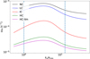 |
Fig. 1 Theoretical linear growth rate as a function of the horizontal wavenumber in the presence of a magnetic field (θ = 10°). The black curves indicate the asymptotic limits corresponding to the fully uncoupled and fully coupled regimes. The colored curves show intermediate coupling cases for two different assumptions on the variation of the collision frequency across the interface. The dashed bands mark the ranges of wavelengths injected in the simulations, illustrating how the numerical experiments sample the different coupling regimes predicted by linear theory. |
3 Verification of the linear theory
The aim of this section is to verify that our numerical set-up correctly reproduces the predictions of the linear Rayleigh-Taylor theory in all configurations relevant to this work (hydrodynamic, single-fluid MHD, and bi-fluid). We proceed gradually, beginning with the definition and validation of the diagnostic used to measure the instability growth, and then increasing the physical complexity step by step. The linear theory developed in Paper I relied on the simplifying assumption that the ion-neutral and neutral-ion collision frequencies were identical on both sides of the density interface. While this choice allowed for a compact analytical formulation, it is not strictly consistent with the numerical implementation used in the present work, where the conserved quantity is the drag coefficient rather than the collision frequency itself. As a result, the collision frequencies naturally vary across the interface in proportion to the local density contrast. In order to ensure a physically consistent comparison between the analytical predictions and the numerical simulations, we relax this assumption and allow the collision frequencies to differ on either side of the interface. We show in Appendix A that this modification does not introduce any new qualitative regime of instability. Instead, it primarily results in a renormalisation of the effective coupling strength at intermediate wavelengths, while leaving the uncoupled and fully coupled asymptotic limits unchanged. The analytical framework of Paper I therefore remains fully applicable, provided that the coupling strength is interpreted in terms of an effective collision frequency.
3.1 Hydrodynamic reference: Compressibility check
The theoretical predictions used throughout this work are based on the incompressible linear analysis of Paper I, while the simulations solve the fully compressible equations. It is therefore necessary to assess whether compressibility may significantly alter the linear growth rates in the parameter regime explored here. Following Díaz et al. (2012), a convenient estimate is provided by the dimensionless ratio gL/cs2, where L is the characteristic perturbation wavelength and cs the sound speed. When gL/cs2 ≪ 1, pressure adjusts rapidly compared to buoyancy-driven motions, and the instability behaves effectively incom-pressibly. Using the largest wavelength present in our simulations, we obtain the conservative estimate
 (15)
(15)
indicating that compressibility effects should remain weak during the linear stage. This expectation is confirmed quantitatively by comparing incompressible and compressible hydrodynamic growth rates for a representative wavelength Lx/4.
The incompressible growth rate ωth,incomp is obtained from the dispersion relation derived in Paper I, while the compressible growth rate ωth,comp is computed using the analytical expression of Díaz et al. (2012) (their Eq. (30)), evaluated for the same physical parameters (density contrast, gravity, and wavelength): ωth,comp = 6.94 × 10 4 s−1,ωth,incomp = 7.02 × 10 4 s−1 which differ by less than 2%. In the remainder of this work, the incompressible dispersion relation is therefore used as a reference framework to interpret the simulations. It is not intended to reproduce the detailed temporal evolution of the compressible system, but to capture the correct ordering of growth rates across wavelengths and coupling regimes. Small temporal offsets between theory and simulations are therefore expected. Given that the smallest injected modes are resolved by ~71 grid points, numerical diffusivity is not expected to significantly affect the linear growth. In addition, the good agreement with the theoretical linear growth rates further indicates that numerical diffusion remains subdominant compared to physical effects. The remaining discrepancy is therefore attributed to weak compressibility and transient initialisation effects.
3.2 Diagnostic tool: Finger-bubble height in the linear and weakly non-linear regimes
In order to quantify the evolution of the Rayleigh-Taylor instability in a way that is robust and comparable across all physical configurations explored in this work (HD, MHD, and bi-fluid), we follow the vertical penetration of both the rising light-fluid bubbles and the descending heavy-fluid spikes (fingers). Our pri-mary observable is the horizontally averaged heavy-fluid fraction as a function of height,
 (16)
(16)
where fh is the local mass fraction of heavy fluid. From ( fh)(z, t) we define two characteristic interface positions: the bubble position zb (t) as the lowest height in the upper half for which the heavy fluid is still present, and the finger position zF(t) as the greatest height in the lower half for which light fluid is still present, using fixed thresholds flow and fhigh (here flow = 0.01 and fhigh = 0.99). In practice, zf (t) is obtained from the crossings of (fh)(z, t) = flow on the z < 0 side (finger penetration), while zb(t) is obtained from the crossings of (fh)(z, t) = fligh on the z > 0 side (bubble rise). We then define the bubble-finger height
 (17)
(17)
which directly measures the thickness of the developing mixing region in a way that is insensitive to a drift of the mean interface position. This diagnostic is widely used in RT studies (e.g. Stone & Gardiner 2007a).
3.3 Linear validation with multiple injected wavelengths
We now validate the linear regime of the instability in a controlled multi-wavelength setting, both in the single-fluid MHD limit and in the bi-fluid framework, before turning to non-linear and multi-scale effects. We independently inject several wavelengths and analyse their early-time evolution with the diagnostic of Sect. 3.2. In all simulations, the initial interface displacement is prescribed with a controlled amplitude proportional to the injected wavelength, h0 = ελ (here e ≈ 1/3), so that all runs start from the same dimensionless configuration. We analyse the normalised height h(t)/h0 and normalise time by the theoretical linear growth rate ωth associated with each wavelength, defining t̄ = ωtht. In the linear regime, the correct theory or diagnostic behaviour therefore implies h/h0 ∝ exp(t̄) and collapse of curves across different wavelengths when plotted as a function of the scaled time t. The extent of the linear regime being not strictly identical across configurations, even after normalisation by ωth, it is identified independently in each case as the interval over which the curves follow a clear exponential trend in semi-logarithmic representation.
We first consider the single-fluid MHD configuration obtained by setting the neutral-ion collision frequency to zero (νnc = 0), with a uniform magnetic field and plasma beta β = 3 × 10². Three wavelengths are selected so as to sample distinct regions of the theoretical growth rate curve, and each wavelength is injected individually in otherwise identical runs. The resulting evolution of h/h0 is shown in Fig. 2.
In the linear regime (0.5 ≲ t̄ ≲ 2), the three curves collapse and appear as straight lines in semi-logarithmic representation, indicating that the exponential growth rates measured in the simulations are consistent with the theoretical predictions. Normalising time by ωth does not modify the exponential behaviour, but rescales the time axis so that different wavelengths can be compared on the same dimensionless basis. A small systematic offset is nevertheless visible at early times (t ≲ 0.5), where the initial perturbation has not yet relaxed onto a pure growing eigenmode. This transient phase contains non-modal contributions, explaining the departure from the ideal exponential behaviour. This validates both the single-fluid dispersion relation and the consistency of the height diagnostic across spatial scales. At later times, the curves naturally deviate from a common exponential as non-linear effects develop, as expected when the interface displacement becomes comparable to the mode scale.
We then perform the same validation in the bi-fluid model in a representative intermediate-coupling regime (IC), where ionneutral interactions are significant but do not trivially enforce a single effective fluid. The same three wavelengths are injected with the same dimensionless initial amplitude h0/λ, and time is normalised by the theoretical bi-fluid growth rate ωth for each wavelength and coupling strength. Figure 2b shows that the curves again collapse tightly in the linear regime, indicating that the bi-fluid dispersion relation correctly predicts the scale dependence of the linear growth and that the numerical coupling implementation reproduces the expected exponential stage. As in the single-fluid case, a slight early-time deviation from the theoretical exponential curve is observed, reflecting the finite-amplitude initialisation and the adjustment toward the linear eigenmode. The exponential slopes, however, remain consistent with theory over the identified linear interval. For completeness, we note that in strictly uncoupled bi-fluid runs (νnc = 0) one may observe a small systematic early-time offset even after normalisation by ωth; since the exponential slopes remain correct, this effect is best interpreted as a transient adjustment of the initial conditions rather than as an error in the growth rate itself. Importantly, this delay is absent in the IC configuration shown here, suggesting that even moderate coupling suppresses such early relaxation effects. Overall, the multi-wavelength collapse in both figures provides a stringent validation of the linear theory and of the diagnostic pipeline used throughout the remainder of the paper.
The results show that the linear growth in our simulations is well reproduced by the incompressible dispersion relation of Paper I, within the expected limitations from compressibility and finite-amplitude initialisation. Growth rates and mode ordering are consistently recovered across wavelengths and coupling regimes. Small early-time deviations are due to transient adjustment effects rather than inaccuracies in the theoretical growth rates. This validates the numerical set-up and ensures that the deviations discussed later arise from non-linear and ambipolar diffusion effects.
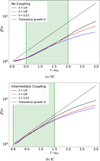 |
Fig. 2 Linear stage. Normalised finger-bubble height h/h0 as a function of the reduced time t̄ = ωtht for three injected wavelengths. The curves show the numerical results, and the solid green line corresponds to the theoretical exponential growth. The shaded green region indicates the time interval identified as the linear growth regime. Top panel: nocoupling (NC) case. Bottom panel: intermediate-coupling (IC) case. |
 |
Fig. 3 Quadratic scaling of the mixing height in the single-fluid case (νnc = 0). Each colour represents a different value of the perturbation wavelength. |
4 Non-linear analysis
We now examine the non-linear evolution of the Rayleigh-Taylor instability and the role of ambipolar diffusion beyond the linear regime. The analysis starts from single-mode perturbations to isolate non-linear effects, and is then extended to multi-wavelength configurations in both hydrodynamic and magnetised regimes.
4.1 One wavelength
In the non-linear stage of the Rayleigh-Taylor instability, the growth of the mixing layer is often described by the quadratic law (Sharp 1984; Dimonte et al. 2004)
 (18)
(18)
where A is the Atwood number, g the gravitational acceleration, and α a dimensionless coefficient characterising the effective non-linear growth. This scaling is commonly associated with a self-similar regime in which the dynamics is governed by a single macroscopic length scale h(t) and a characteristic velocity U ~ ḣ, while the detailed flow physics is absorbed into the value of α. In the following, this quadratic scaling is therefore used as a reference framework to assess how ambipolar diffusion modifies the non-linear evolution, rather than as an a priori universal growth law.
We first consider the uncoupled case (νnc = 0), which provides a reference single-fluid behaviour. Figure 3 shows the dimensionless mixing height h/λ as a function of the rescaled time t ωth, where ωth is the linear growth rate predicted by the two-fluid linear analysis. For all considered wavelengths, the curves are approximately linear, confirming the quadratic growth of the mixing layer, and their slopes remain comparable over a broad range of wavelengths, in agreement with previous numerical studies. At the shortest wavelengths, a tendency toward saturation is observed at small scales, which can be attributed to enhanced dissipation and finite resolution effects. Overall, in the absence of coupling, the quadratic model provides an accurate and robust description of the non-linear growth in our 2D simulations. Before turning to the coupled regimes, it is important to stress that the quadratic model in Eq. (18) should be regarded as an effective description rather than a strict law, especially in two-dimensional configurations. As emphasised by Kalluri & Hillier (2025), self-similarity in Rayleigh-Taylor mixing does not necessarily imply an exactly quadratic growth at all times, but rather the emergence of a regime controlled by a single macroscopic length scale, in which suitably defined dimensionless coefficients remain approximately constant. In 2D, the coexistence of direct and inverse cascades and the persistence of large-scale coherent structures make this regime intrinsically less robust than in three dimensions, so that temporal modulations of the effective growth rate are expected even in the absence of additional physics. In this context, the parameter α should be interpreted as a time-averaged measure of the non-linear growth efficiency, whose applicability may be limited when additional mechanisms interfere with the inertial-buoyancy balance.
When ambipolar coupling is introduced, the non-linear evolution departs more profoundly from the quadratic reference. As shown in Fig. 4, the ambipolar regime is characterised by a pronounced curvature of the growth curves, indicating a subquadratic evolution over an extended time interval. The mixing height therefore grows more slowly than predicted by Eq. (18), reflecting a strong reduction of the instantaneous growth rate compared to the uncoupled case. At later times, the curves tend to straighten again, suggesting a gradual recovery of a quasiquadratic behaviour, but with a significantly reduced effective coefficient. This behaviour shows that ambipolar diffusion does not simply renormalise the quadratic law through a smaller constant, but instead induces a genuinely time-dependent growth process. The failure of the quadratic description in the ambipolar regime can be understood from a simple physical argument. In the classical single-fluid picture, the buoyancy power injected into the flow is assumed to be directly converted into bulk kinetic energy at the scale of the mixing layer, so that the non-linear dynamics can be closed in terms of the single macroscopic length scale h(t). In a partially ionised medium, however, buoyancy initially accelerates only the charged component, while neutrals are entrained progressively through ion-neutral collisions. During this phase, a finite slip velocity develops and a non-negligible fraction of the injected buoyancy power is transferred into relative ion-neutral motion and dissipated by drag on a characteristic coupling timescale. As a result, the instantaneous growth rate of the mixing layer depends not only on h(t), but also on the time-dependent state of coupling between the two fluids, preventing the closure of the growth law in terms of h alone.
To interpret the departure from a purely quadratic growth observed in Fig. 4a, we consider a minimal two-fluid model in which buoyancy acts only on the charged component, while ions and neutrals exchange momentum through linear ion-neutral drag. The model assumes spatially averaged velocities, a constant density ratio χ ≡ ρc/ρn, and neglects pressure gradients, turbulent transport, and spatial intermittency. Its purpose is not to provide a quantitative description of the non-linear Rayleigh-Taylor instability, but to isolate the dynamical consequences of time-dependent ion-neutral coupling.
This model does not describe the detailed evolution of the interface, but rather a spatially averaged bulk dynamics of the two fluids. It should be understood as a minimal Lagrangian description, in which the characteristic velocity is identified with the large-scale growth of the mixing layer:
 (19)
(19)
 (20)
(20)
where νnc is the neutral-on-charge collision frequency and Δu ≡ Uc - Un is the slip velocity. Subtracting the two equations yields a closed evolution equation for the drift:
 (21)
(21)
which relaxes exponentially on the coupling timescale τc = [νnc(1 + χ)]−1. Summing the momentum equations gives the total momentum balance,
 (22)
(22)
from which the center-of-mass velocity grows linearly as  .
.
Combining these two results, the charged velocity can be written explicitly as the sum of a center-of-mass contribution and a transient drift term. Identifying the charged bulk velocity with the growth rate of the mixing layer, Uc ≃ ḣ, one obtains an analytical expression for the mixing height:
![Mathematical equation: h(t)-h_0=\frac{\mathcal{A}g\,\chi}{2(1+\chi)}\,t^2+\frac{\mathcal{A}g}{\nu_{\rm nc}^2(1+\chi)^3}\left[(1+\chi)\nu_{\rm nc}t-\bigl(1-e^{-(1+\chi)\nu_{\rm nc}t}\bigr)\right].](/articles/aa/full_html/2026/06/aa59496-26/aa59496-26-eq24.png) (23)
(23)
Introducing the reduced time t̃ ≡ vnc t, the mixing height can be rewritten in dimensionless form as
![Mathematical equation: h\left(\dfrac{\tilde t}{\nu_{\rm nc}}\right)-h_0 = \frac{\mathcal{A}g}{\nu_{\rm nc}^2} \left[ \frac{\chi}{2(1+\chi)}\,\tilde t^{\,2} + \frac{(1+\chi)\tilde t-\bigl(1-e^{-(1+\chi)\tilde t}\bigr)}{(1+\chi)^3} \right].](/articles/aa/full_html/2026/06/aa59496-26/aa59496-26-eq25.png) (24)
(24)
In this form, the growth law depends explicitly only on the reduced elapsed time νnct, making clear that the non-linear evolution is governed by the relative ordering of the buoyancy timescale and the ion-neutral coupling time.
At early times, νnct ≪ 1, ions and neutrals are effectively decoupled and the charged component accelerates freely, recovering the classical quadratic growth h ∝ Agt2. In the opposite limit, νnc t ≫ 1, ions and neutrals are locked together and the system behaves as a single fluid of total inertia, yielding h ∝ Ag(ρc/ρtot) t2. The intermediate regime vnct ~ 1 corresponds to a transient phase during which neutrals are progressively entrained by drag, leading to a time-dependent increase of the effective inertia and a reduced instantaneous growth rate.
This behaviour is illustrated in Fig. 4b, where the theoretical prediction for h/λ is plotted as a function of (t ∙ ωth)2 for weakly (LC), intermediately (IC), and strongly (HC) coupled cases. The model reproduces the pronounced curvature of the IC curve, as well as the reduced asymptotic prefactor in the HC limit, in close qualitative agreement with the simulations. The remaining offset in the normalisation of h/λ reflects the fact that the present model does not include the phenomenological efficiency factor usually introduced in self-similar RT growth, such that h = α Ag t2 with α < 1. As a result, the model correctly captures the temporal evolution but not the absolute normalisation of the mixing height. Importantly, the intermediate-coupling regime does not represent a breakdown of self-similar behaviour, but rather a modified form of self-similarity in which the growth law contains both quadratic and linear contributions. The linear term reflects the finite time required for momentum transfer between the two fluids and the associated evolution of the effective inertia of the mixing layer. The observed sub-quadratic growth therefore arises naturally from the intrinsic two-fluid dynamics, without invoking additional non-linear saturation mechanisms.
 |
Fig. 4 Quadratic scaling of the mixing height for the No-coupling, Low-coupling, Intermediate-coupling, and High-coupling cases (NC, LC, IC, HC) for λ = 1/4Lx. Top Panel: simulation result. Bottom panel: theoretical evolution, predicted by the local two-fluid simplified model. |
 |
Fig. 5 Snapshots of the charge density ρc in hydrodynamic simulations with multi-wavelength initial perturbations, extracted at an equivalent non linear stage defined by a fixed normalised mixing layer thickness, ∆h/Lx ≃ 0.35. From left to right, the panels show increasing coupling strength (α = 0, weak, intermediate, and strong coupling). All snapshots are shown using the same spatial window and colour scale. The density of the charge fluid ρc is given in units of the ρc1, the lighter fluid. |
4.2 Multi-wavelength regime: Hydrodynamic reference
In the multi-wavelength configurations, the interface perturbation is constructed as a broadband superposition of modes,
 (25)
(25)
where N is the number of excited modes and nosc sets the largest injected wavelength. The coefficients ci and phases φi are drawn from uniform random distributions, with ci ∈ [−1,1] and φi ∈ [0,2π], and are fixed across all simulations to ensure reproducibility. We first consider the hydrodynamic configurations as a reference for the non-linear evolution under multi-wavelength perturbations. All comparisons are performed at an equivalent non-linear stage defined by a fixed normalised mixing layer thickness, Δh/Lx ≃ 0.35.
Figure 5 illustrates the non-linear morphology of the mixing layer in the hydrodynamic multi-wavelength simulations at a fixed normalised thickness, Δh/Lx ≃ 0.35, it shows snapshots of the charge density ρc for increasing coupling strength. In the uncoupled case (α = 0), the interface is dominated by a small number of large-scale structures. The initially broadband perturbation rapidly evolves toward coherent bubbles and fingers that undergo efficient lateral merging, leading to extended plumes and a relatively smooth mixing layer. As the coupling strength increases, the morphology is progressively modified. For weak coupling, the global organisation remains close to the uncoupled reference, although small-scale corrugations and secondary structures become more visible along the sides of the plumes. In contrast, the intermediate-coupling regime exhibits a markedly different behaviour: at the same mixing height, the interface is significantly more fragmented, with numerous thin fingers and strongly reduced lateral coalescence. Large-scale plumes fail to emerge, and the mixing region retains a highly structured appearance down to smaller spatial scales. In the strongly coupled regime, the interface recovers a smoother and more coherent morphology, with reduced small-scale fragmentation and a renewed tendency toward large-scale organisation. To quantify these morphological differences, we compute onedimensional power spectra of the charge density ρc along the horizontal direction x, evaluated at the same normalised mixing layer thickness. The spectra are obtained using a Welch-averaged estimator (Welch 1967) and normalised by their maximum value to highlight the relative distribution of power across scales.
Figure 6 shows that the redistribution of structures observed in real space is accompanied by clear, systematic changes in spectral content. In the uncoupled case, the power is predominantly concentrated at small wavenumbers, consistent with the dominance of large-scale plumes. As the coupling strength increases, power is progressively shifted toward larger horizontal wavenumbers (i.e. kx), indicating an enhanced contribution from smaller spatial scales at the same mixing height. This redistribution is most pronounced in the intermediate-coupling regime, which exhibits the strongest relative enhancement of high-kx power. In the strongly coupled case, the spectrum departs less markedly from the uncoupled reference, consistent with the partial recovery of large-scale organisation seen in the snapshots.
Taken together, the snapshots and density spectra demonstrate that ion-neutral coupling has a non-monotonic impact on the non-linear, multi-scale organisation of the mixing layer. At fixed Δh/Lx, intermediate coupling is the most effective at inhibiting large-scale coalescence and maintaining power at smaller horizontal scales, while both weak and strong coupling favor the emergence of larger-scale structures. This hydrodynamic reference establishes that ambipolar coupling can fundamentally reorganise the non-linear cascade of structures even in the absence of magnetic forces, providing a baseline for interpreting the magnetised configurations discussed below.
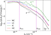 |
Fig. 6 One-dimensional power spectrum of the charge density ρc along the horizontal direction x, computed for the hydrodynamic multiwavelength simulations at a fixed non-linear stage defined by ∆h/Lx ≃ 0.35. The spectra correspond to |

4.3 Multi-wavelength MHD regime
We now shift to 2D MHD simulations with multi-wavelengths. Figure 7 shows snapshots of the charge density ρc for the magnetised simulations at an equivalent non-linear stage, Δh/Lx ≃ 0.35, for increasing values of the coupling parameter α.
At Δh/Lx ≃ 0.35, all magnetised simulations exhibit a fully developed mixing layer whose overall morphology differs markedly from the hydrodynamic reference at the same nonlinear stage. In all MHD cases, the interface appears globally smoother, with a reduced level of small-scale corrugations and fewer secondary structures, consistent with the suppression of short-wavelength features by magnetic tension. In the uncoupled MHD case (α = 0), the mixing layer is organised into well-defined bubbles and fingers, but the interface retains a noticeable degree of fine structure. Small protrusions and lateral modulations are present along the sides of the main plumes, indicating that, in the absence of ion-neutral coupling, the charged component can still sustain a significant level of small-scale variability despite the presence of the magnetic field. For weak coupling, the overall appearance of the mixing layer remains similar, but the interface becomes slightly more regular. The fingers are more uniform in shape, and the smallest-scale features observed in the uncoupled case are less frequent, suggesting a partial damping of secondary structures as the coupling increases. In the intermediate-coupling regime (α = 7.5 × 10²⁰), the morphology becomes noticeably more coherent. The dominant bubbles are comparatively straight and elongated, with smooth lateral boundaries and very limited internal substructure. The interface is dominated by a small number of clean, well-defined plumes, and fine-scale corrugations are strongly reduced. In the strongly coupled case, the mixing layer remains globally similar in extent, but the interface recovers a degree of complexity. While large-scale bubbles persist, thin fingers and localised distortions reappear along the interface, leading to a more intricate and less uniform morphology than in the intermediate case. This indicates that the influence of coupling on the non-linear organisation of the flow is not monotonic with α.
To further quantify the spatial organisation of the flow, we compute the one-dimensional power spectra of the charge density along the horizontal direction at the same non-linear stage, Δh/Lx ≃ 0.35. The spectra, shown in Fig. 8, are obtained using a Welch-averaged estimator applied within the mixing layer. Despite the morphological differences observed in real space, the spectra exhibit no significant dependence on the coupling strength over the range of resolved scales. In particular, both the spectral slope and the relative distribution of power across horizontal wavenumbers remain remarkably similar between the different MHD runs. This indicates that, at this advanced stage of the non-linear evolution, the global statistical distribution of power in the charge density is largely insensitive to the value of α, even though the geometry of individual bubbles and fingers continues to vary.
To identify the mechanisms governing the non-linear reorganisation of the mixing layer in the magnetised simulations, we examine spatial maps of the dominant force densities at a fixed non-linear stage, Δh/Lx ≃ 0.35. Figure 9 shows, for each coupling regime, the Lorentz force acting on the charged component and the ion-neutral drag force acting on the neutrals, computed from the instantaneous fields.
The top row displays the magnitude of the Lorentz force density,

together with magnetic field lines (cgs units). The Lorentz force is strongly localised along the mixing interface, with enhanced amplitudes near bubble and finger edges and in regions of strong field-line curvature. This localisation indicates a tension-dominated response, acting through thin layers that redistribute momentum along the interface rather than throughout the volume. The bottom row shows the magnitude of the ion-neutral drag force, Rn = αρcρn (vc - vn), with streamlines of the relative velocity Δv = vc - vn. In contrast to fL, the drag force extends over a larger fraction of the mixing region and highlights zones of strong inter-fluid slip, particularly in compressive and shear regions around plume edges. These maps reveal a clear separation of roles: magnetic stresses are localised and associated with field-line curvature, while ion-neutral drag is more spatially extended and governs dissipation through drift. This does not imply a local balance between the two forces, as pressure gradients and inertial terms remain dominant in the momentum equation. The Lorentz force also contributes to energy exchange via the work term vc ∙ fL, enabling local conversion of magnetic energy into kinetic energy.
To complement the local force maps, we now examine the global energy pathways that govern the non-linear evolution of the mixing layer. Figure 10 shows the cumulative gravitational energy injection  , with Pg = ρcvc,zg, together with the cumulative ion-neutral drag dissipation
  , where Dkin = αρcρn|vc - vn|2, both represented as functions of the normalised mixing layer thickness Δh/Lx. A robust result is that the Intermediate-coupling (IC) regime stands out energetically: at a given non-linear stage, IC simultaneously reaches a maximum of drag-related dissipation and a minimum of gravitational energy content. This behaviour is physically expected, since the gravitational source term scales with the charged velocity, Pg ∝ vc,z, so that efficient momentum exchange with neutrals reduces the charged flow speed and limits the gravitational energy retained in the charged component, while maximising the relative slip between the two fluids and therefore the drag dissipation. As a result, the gravitational energy injected into the system is converted most efficiently into ion-neutral drift in the IC regime. In contrast, the weakly coupled (LC) and strongly coupled (HC) regimes display comparable global energetic behaviour, both characterised by lower dissipation efficiencies. In the LC case, the charged fluid evolves almost independently of the neutrals, limiting the development of significant inter-fluid drift, whereas in the HC limit the two fluids are nearly locked together, suppressing relative motion and reducing drag dissipation. The HC-limit case further exhibits the largest gravitational energy content, consistent with the persistence of higher charged velocities when slip is strongly inhibited. It is important to emphasise that these simulations are performed in an open vertical configuration, so that the total energy budget is not strictly closed and energy can enter or leave the domain through the boundaries. For this reason, the present analysis does not aim at establishing a strict conservation law, but rather at comparing how gravitational energy is redistributed between physical channels across coupling regimes. In addition, although not shown explicitly in the cumulative diagnostics, the magnetic channel contributes to the energy redistribution through the work of the Lorentz force, vc ∙ fL, which transfers energy between magnetic stresses and bulk kinetic motions. This contribution is spatially localised, as discussed in Fig. 9, and complements the dominant drag-mediated dissipation channel. From this perspective, the global trends reinforce the interpretation suggested by the local force maps: the non-linear organisation of the mixing layer is controlled not by the total amount of injected gravitational energy, but by how efficiently this energy is redirected into ion-neutral drift versus magnetic stresses.
We deliberately limit the analysis to this stage of the nonlinear evolution and do not attempt to characterise a late-time saturated regime. In magnetised Rayleigh-Taylor configurations, saturation does not necessarily coincide with the onset of fully developed turbulence, as is often assumed in purely hydrodynamic studies, but may instead result from a geometry-driven or force balance-driven arrest that depends on the wavelength content and on the horizontal magnetic component Bx. Moreover, because the vertical boundaries act as open reservoirs, the global energy budget is not strictly closed, so that extending the energy-based analysis to later times would require a dedicated control-volume approach tied to the mixing layer thickness or fully three-dimensional simulations with carefully designed boundary conditions. For these reasons, we focus here on the physically robust regime where the non-linear organisation of the mixing layer can be unambiguously related to the partition of injected gravitational power between ion-neutral drift and magnetic stresses.
 |
Fig. 7 Snapshots of the charge density ρc in MHD simulations with multi-wavelength initial perturbations, extracted at an equivalent non-linear stage defined by a fixed normalised mixing layer thickness, ∆h/Lx ≃ 0.35. From left to right, the panels correspond to increasing coupling strength: α = 0, weak coupling, intermediate coupling, and strong coupling. All snapshots are shown using the same spatial window and colour scale. The density of the charge fluid ρc is given in units of the ρc1, the lighter fluid. |
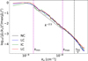 |
Fig. 8 One-dimensional power spectrum of the charge density ρc along the horizontal direction x, computed for the magnetised multiwavelength simulations at an equivalent non-linear stage defined by ∆h/Lx ≃ 0.35. All spectra were obtained using the same spectral procedure and are normalised by their maximum value. The different curves correspond to increasing ion-neutral coupling strength and are labelled NC, LC, IC, and HC (see Sect. 3). The vertical dashed lines indicate the minimum and maximum injected wavenumbers, as well as half the Nyquist limit. |
5 Conclusion
In this work, we have investigated the non-linear development of the Rayleigh-Taylor instability in a partially ionised plasma, with a particular emphasis on the role of ambipolar diffusion in the presence of an oblique magnetic field. Building on the linear analysis presented in Paper I, we combined highresolution two-fluid simulations with self-consistent diagnostics in order to quantify how ion-neutral coupling modifies both the growth and the morphology of the mixing layer beyond the linear regime. We first demonstrated that our numerical setup accurately reproduces the predictions of the linear theory across hydrodynamic, single-fluid MHD, and bi-fluid configurations. Using a finger-bubble diagnostic, we confirmed that the theoretical growth rates are recovered for a wide range of wavelengths and coupling strengths, and that compressibility effects remain negligible in the parameter regime considered. This validation step provides a robust foundation for the nonlinear analysis. In the non-linear regime, we showed that while the classical quadratic scaling of the mixing height, h (t) ∝ A g t2, remains a useful global description, it fails to capture important time-dependent features induced by ambipolar diffusion. By introducing a morphology-based alignment procedure based on a fixed normalised mixing height h/λ, we were able to perform meaningful comparisons between simulations with vastly different linear growth rates. This approach revealed a characteristic inflected behaviour of the mixing-layer evolution when ambipolar diffusion becomes dynamically important. In particular, we identified a specific coupling regime in which ambipolar diffusion produces a non-trivial modification of the non-linear dynamics. After synchronisation at an equivalent morphological stage, the evolution exhibits a transient phase of enhanced growth relative to the uncoupled reference, followed by a pronounced slowdown that leads to a reduced mixing efficiency at later times. The ratio of mixing heights between coupled and uncoupled runs asymptotically approaches a value significantly below unity, of order ~0.7 for the most affected cases. This behaviour demonstrates that ambipolar diffusion does not simply rescale the non-linear growth coefficient, but instead reshapes the temporal evolution of the instability in a genuinely time-dependent manner.
We further showed that these effects persist when the interface is perturbed over a broad range of wavelengths. In the multi-mode regime, ambipolar diffusion strongly modifies the morphology of the mixing layer, inhibiting large-scale plume coalescence and promoting a more fragmented interface at intermediate coupling. Although one-dimensional power spectra of the charge density at fixed non-linear stage do not reveal a clear change in global scaling laws, they nonetheless confirm that the statistical distribution of power across horizontal wavenumbers remains largely insensitive to coupling. This absence of a strong spectral signature indicates that the observed morphological differences are not associated with a simple spectral cutoff, but rather reflect a local and geometrical reorganisation of the flow. A more direct physical interpretation emerges from the analysis of energy conversion channels. By comparing the relative contributions of gravitational injection, Lorentz work, and ion-neutral drag dissipation at equivalent non-linear stages, we showed that ambipolar diffusion primarily acts by redistributing energy locally within the mixing layer. In particular, the fraction of gravitational power converted into ion-neutral drift reaches a maximum at intermediate coupling, while the global contribution of magnetic stresses remains comparatively modest and weakly dependent on the coupling strength. This non-monotonic behaviour provides a natural explanation for the enhanced smoothness and coherence observed in the intermediate regime, where the drift efficiently extracts energy from the flow without completely suppressing the development of large-scale structures.
Taken together, these results demonstrate that ambipolar diffusion introduces a bounded regime of non-linear behaviour in which the Rayleigh-Taylor instability departs qualitatively from the standard self-similar picture. Rather than acting as a simple effective diffusivity, ambipolar coupling produces an early acceleration followed by a sustained non-linear braking, accompanied by a redistribution of energy between bulk motions, magnetic stresses, and differential ion-neutral drift. The resulting morphology reflects a delicate balance between magnetic tension, which suppresses short-wavelength perturbations, and ambipolar diffusion, which locally reorganises the flow through slip-mediated dissipation. From a methodological standpoint, this work highlights the importance of morphology-based synchronisation when comparing non-linear evolutions across different physical regimes. Aligning simulations at a fixed normalised mixing height provides a robust framework to disentangle genuine physical effects from trivial timing differences associated with distinct linear growth rates. This approach is particularly well suited to multi-fluid systems, where additional timescales associated with coupling can strongly affect the apparent nonlinear evolution. Finally, while the present study focuses on idealised two-dimensional configurations, the mechanisms identified here are expected to play an important role in a wide range of astrophysical environments where partially ionised plasmas and magnetic fields coexist, such as molecular clouds, supernova remnants, or the interfaces of expanding HII regions. Extensions to three dimensions, as well as to regimes including additional physical ingredients such as cooling, stratification, or cosmic-ray feedback, constitute natural directions for future work. The results presented here provide a physically grounded reference for such studies and emphasise that ambipolar diffusion can qualitatively alter the non-linear outcome of classical hydromagnetic instabilities.
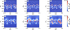 |
Fig. 9 Spatial organisation of force densities in the magnetised multi-wavelength simulations at a fixed non-linear stage Δh/Lx ≃ 0.35. Top row: magnitude of the Lorentz force acting on the charged fluid, |

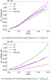 |
Fig. 10 Global energy pathways as functions of the normalised mixing layer thickness Δh/Lx for different ion-neutral coupling strengths. The intermediate-coupling regime maximises the conversion of gravitational energy into drag-related dissipation, while both weak and strong coupling lead to reduced dissipation efficiency. |
Acknowledgements
The authors are grateful to K. Ferrière, P. Lesaffre, F. Boulanger, O. Berné for fruitful discussions. We also thank A. Cogez for his contribution during his internship. This work was supported by the Thematic Action “Programme National Physique Stellaire” (PNPS) of INSU Programme National “Astro”, with contributions from CNRS Physique & CNRS Chimie, CEA, and CNES.
References
- Arons, J., & Lea, S. M. 1976, ApJ, 207, 914 [Google Scholar]
- Ascher, U. M., Ruuth, S. J., & Spiteri, R. J. 1997, Appl. Numer. Math., 25, 151 [CrossRef] [MathSciNet] [Google Scholar]
- Braileanu, B. P., & Keppens, R. 2022, A&A, 664, a55 [Google Scholar]
- Bucciantini, N., Amato, E., & Del Zanna, L. 2004, A&A, 423, 253 [NASA ADS] [CrossRef] [EDP Sciences] [Google Scholar]
- Callies, E., Guillet, V., Marcowith, A., Meliani, Z., & Lesaffre, P. 2025, A&A, 698, A147 [NASA ADS] [CrossRef] [EDP Sciences] [Google Scholar]
- Carlyle, J., & Hillier, A. 2017, A&A, 605, A21 [NASA ADS] [CrossRef] [EDP Sciences] [Google Scholar]
- Chandrasekhar, S. 1961, Hydrodynamic and Hydromagnetic Stability (Oxford: Oxford University Press) [Google Scholar]
- Changmai, M., Jenkins, J. M., Durrive, J. B., & Keppens, R. 2023, A&A, 672, A152 [NASA ADS] [CrossRef] [EDP Sciences] [Google Scholar]
- Colella, P., & Woodward, P. R. 1984, J. Comput. Phys., 54, 174 [NASA ADS] [CrossRef] [Google Scholar]
- Cook, A. W., Cabot, W. H., & Miller, P. L. 2004, J. Fluid Mech., 511, 333 [Google Scholar]
- Díaz, A. J., Soler, R., & Ballester, J. L. 2012, ApJ, 754, 41 [Google Scholar]
- Díaz, A. J., Khomenko, E., & Collados, M. 2014, A&A, 564, A97 [NASA ADS] [CrossRef] [EDP Sciences] [Google Scholar]
- Dimonte, G., Youngs, D., Dimits, A., et al. 2004, Phys. Fluids, 16, 1668 [NASA ADS] [CrossRef] [Google Scholar]
- Fermi, E., & von Neumann, J. 1953, Los Alamos Scientific Laboratory Report [Google Scholar]
- Hester, J. J., et al. 1996, ApJ, 456, 225 [Google Scholar]
- Hillier, A. 2016, PhD thesis, University of St Andrews, UK [Google Scholar]
- Isobe, H., Miyagoshi, T., Shibata, K., & Yokoyama, T. 2005, Nature, 434, 478 [Google Scholar]
- Jun, B.-I., & Norman, M. L. 1996, ApJ, 465, 800 [Google Scholar]
- Jun, B.-I., Norman, M. L., & Stone, J. M. 1995, ApJ, 453, 332 [Google Scholar]
- Kalluri, M. T., & Hillier, A. 2025 [arXiv:2510.27053] [Google Scholar]
- Khomenko, E., Vitas, N., Collados, M., & Modestov, M. 2025, A&A, 697, A29 [NASA ADS] [CrossRef] [EDP Sciences] [Google Scholar]
- Miyoshi, T., & Kusano, K. 2005, J. Comput. Phys., 208, 315 [NASA ADS] [CrossRef] [Google Scholar]
- Popescu Braileanu, B., Lukin, V. S., Khomenko, E., & de Vicente, Á. 2021a, A&A, 646, A93 [NASA ADS] [CrossRef] [EDP Sciences] [Google Scholar]
- Popescu Braileanu, B., Lukin, V. S., Khomenko, E., & de Vicente, Á. 2021b, A&A, 650, A181 [NASA ADS] [CrossRef] [EDP Sciences] [Google Scholar]
- Popescu Braileanu, B., Lukin, V. S., & Khomenko, E. 2023, A&A, 670, A31 [NASA ADS] [CrossRef] [EDP Sciences] [Google Scholar]
- Rayleigh, L. 1883, Proc. London Math. Soc., 14, 170 [MathSciNet] [Google Scholar]
- Ristorcelli, J. R., & Clark, T. T. 2004, J. Fluid Mech., 507, 213 [Google Scholar]
- Robinson, K., Dursi, L. J., Ricker, P. M., et al. 2004, ApJ, 601, 621 [Google Scholar]
- Ruszkowski, M., Enßlin, T. A., Brüggen, M., & Heinz, S. 2007, MNRAS, 378, 662 [NASA ADS] [CrossRef] [Google Scholar]
- Ruuth, S. J., & Spiteri, R. J. 2002, J. Sci. Comput., 17, 211 [CrossRef] [Google Scholar]
- Sharp, D. H. 1984, Phys. Rep., 101, 221 [Google Scholar]
- Soler, R., & Ballester, J. L. 2022, Front. Astron. Space Sci., 9, 789083 [Google Scholar]
- Stone, J. M., & Gardiner, T. 2007a, ApJ, 671, 1726 [NASA ADS] [CrossRef] [Google Scholar]
- Stone, J. M., & Gardiner, T. A. 2007b, ApJ, 671, 1726 [NASA ADS] [CrossRef] [Google Scholar]
- Stone, J. M., & Gardiner, T. A. 2007c, Phys. Fluids, 19, 094104 [NASA ADS] [CrossRef] [Google Scholar]
- Taylor, G. I. 1950, Proc. R. Soc. London. Ser. A, 201, 192 [Google Scholar]
- Vickers, E., Ballai, I., & Erdélyi, R. 2020, A&A, 634, A96 [NASA ADS] [CrossRef] [EDP Sciences] [Google Scholar]
- Vigoureux, G., Flagey, N., Boulanger, F., et al. 2026, A&A, 707, A374 [NASA ADS] [CrossRef] [EDP Sciences] [Google Scholar]
- Wang, Y.-M., & Nepveu, M. 1983, A&A, 118, 267 [Google Scholar]
- Welch, P. 1967, IEEE Trans. Audio Electroacoustics, 15, 70 [Google Scholar]
MPI-AMRVAC v3.0-289-g034bdf3d (commit 034bdf3d), compiled and run with OpenMPI 5.0.8.
Appendix A Discussion of Paper I
In Paper I, the analytical dispersion relation was derived under the simplifying assumption that the ion-neutral and neutral-ion collision frequencies were identical on both sides of the density interface. While this assumption facilitates the algebraic treatment of the matching conditions, it is not fully consistent with the numerical prescription adopted in MPI-AMRVAC, where the drag coefficient α is conserved and the collision frequencies scale with the local density. In the numerical model, the collision frequencies are defined as
 (A.1)
(A.1)
so that they vary proportionally to the density of the interacting species. Across an interface separating two homogeneous layers of densities ρ1 and ρ2, we define the density contrast:
 (A.2)
(A.2)
Because the drag coefficient α is constant, the collision frequencies on either side of the interface scale in the same way, yielding
 (A.3)
(A.3)
To account for this asymmetry in the analytical formulation, we introduce the parameter
 (A.4)
(A.4)
In the physically consistent case corresponding to a constant drag coefficient, this parameter is therefore not free, but directly related to the density contrast as
 (A.5)
(A.5)
The case ξ = 1 corresponds to the simplifying assumption adopted in Paper I, where the ion-neutral collision frequency was taken to be uniform across the interface. In that framework, the linear system reduces to the matrix given in Eq. (54), which further simplifies to Eq. (81) when gn = 0, due to additional symmetries arising from the assumption ρc = ρn. In contrast, the case ξ = d considered here reflects the physically consistent variation of the collision frequency with density, as implemented in the numerical model. Because ρc ≠ ρn across the interface, the collision frequencies differ between the two layers, and the simplifications leading to Eq. (81) in Paper I can no longer be applied. As a result, the full matrix structure must be retained, including the additional terms associated with D1 and D2. The matrix should therefore be directly compared to Eq. (54) of Paper I, rather than to its simplified form. :
 (A.6)
(A.6)
with
 (A.7)
(A.7)
 (A.8)
(A.8)
 (A.9)
(A.9)
 (A.10)
![Mathematical equation: m_{1-}&=-\left[i\left(\dfrac{k_x}{\tan\theta}\right)-\dfrac{\Omega}{\sin\theta\,\cac\phiOne}\right]\\](/articles/aa/full_html/2026/06/aa59496-26/aa59496-26-eq42.png) (A.11)
(A.11)
![Mathematical equation: m_{2+}&=-\left[i\left(\dfrac{k_x}{\tan\theta}\right)+\dfrac{\Omega}{\sin\theta\,\sqrt{d}\cac\phiTwo}\right]](/articles/aa/full_html/2026/06/aa59496-26/aa59496-26-eq43.png) (A.12)
(A.12)
![Mathematical equation: \alpha_{1{\rm c}}&\equiv k_x\left[\gc-\left(\cAone^2k\sin^2\theta-\dfrac{\Omega\left(\nunc+\Omega\right)}{k}\right)\right] \ ,\\](/articles/aa/full_html/2026/06/aa59496-26/aa59496-26-eq44.png) (A.13)
(A.13)
![Mathematical equation: \alpha_{2{\rm c}}&\equiv d^{-1}k_x\left[ \gc+\left(d\cAone^2k\sin^2\theta-\dfrac{\Omega\left(\nunc/\xi+\Omega\right)}{k}\right)\right] \ ,\\](/articles/aa/full_html/2026/06/aa59496-26/aa59496-26-eq45.png) (A.14)
(A.14)
 (A.15)
 (A.16)
 (A.17)
 (A.18)
 (A.19)
 (A.20)
 (A.21)
 (A.22)
 (A.23)
Allowing the collision frequencies to vary across the interface modifies the analytical formulation in a controlled but non-trivial way. When ξ ≠ 1, the neutral-ion and ion-neutral collision frequencies explicitly differ on each side of the interface, so that the matching conditions involve distinct dynamical responses in the two layers. As a result, several auxiliary quantities introduced in Paper I, such as the parameters φ1,2 and ψ1,2, acquire an explicit dependence on ξ, and the coefficients entering the interface conditions—in particular αic, βic, γic, δic and their neutral counterparts—must be evaluated using different collision frequencies on either side of the interface. While the overall block structure of the matching matrix is preserved, this asymmetry breaks part of the algebraic simplifications exploited in Paper I, where the coupling could be represented by a single effective parameter. In the present formulation, the coupling enters through several coefficients simultaneously, which makes the dispersion relation less amenable to a compact analytical reduction and renders the interpretation of the coupling regimes less direct from the mathematical expression alone. Nevertheless, the physical structure of the problem remains unchanged: the dispersion relation still connects continuously the limits of vanishing coupling and perfect coupling, and the same asymptotic behaviours are recovered when the collision frequency becomes either negligible or dominant compared to the dynamical timescale.
The practical impact of this modification is illustrated in Fig. A.1, where the linear growth rate is plotted as a function of the wavenumber k for different coupling strengths, comparing the cases ξ = 1 (as assumed in Paper I) and ξ = d, corresponding to a collision frequency variation driven solely by the density contrast across the interface. The uncoupled and fully coupled asymptotic limits are shown for reference and are identical in both cases, confirming that the modification does not alter the fundamental limiting behaviour of the instability. Differences arise primarily at intermediate wavenumbers, where the growth rate obtained with ξ = d is systematically reduced compared to the ξ = 1 case for the same nominal collision frequency. This reduction reflects the asymmetric collision-frequency distribution across the interface: when ξ = d, the coupling strength differs between the two layers, which modifies the relative contribution of each fluid to the linear dynamics and enhances the effective damping at intermediate scales. For practical comparison with the formulation of Paper I, it is convenient to introduce an effective collision frequency νnc,eq defined operationally as the value that minimises the mismatch between the ξ = d dispersion curve and the ξ = 1 curve over a chosen intermediate-k interval. With this definition, the two formulations can be brought into close quantitative agreement without affecting the uncoupled and perfectly coupled limits. The ratio νnc,eq/νnc is not universal: it depends on the density contrast d and, to a lesser extent, on the coupling regime considered. Therefore, the transition from ξ = 1 to ξ = d does not introduce a new qualitative regime of instability, but rather corresponds to a renormalisation of the effective coupling strength when the collision frequencies are allowed to scale consistently with density. The theoretical framework developed in Paper I thus remains fully applicable, provided that collision frequencies are interpreted in terms of an effective coupling when comparing analytical predictions with physically consistent numerical prescriptions.
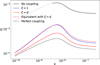 |
Fig. A.1 Linear growth rate as a function of the wavenumber k. The black curves show the two asymptotic limits: the uncoupled case (No coupling) and the perfectly coupled case (Perfect coupling). The blue curve corresponds to the formulation with ξ = 1 used in Paper I, while the red curve shows the physically consistent case ξ = d, where the collision frequencies scale with the density contrast across the interface (constant drag coefficient α). The dashed red curve labelled ‘Equivalent with ξ = d’ shows the ξ = 1 formulation evaluated with an effective collision frequency νnc,eq chosen so as to reproduce the ξ = d dispersion curve over the intermediate-k range. |
All Tables
All Figures
|
Fig. 1 Theoretical linear growth rate as a function of the horizontal wavenumber in the presence of a magnetic field (θ = 10°). The black curves indicate the asymptotic limits corresponding to the fully uncoupled and fully coupled regimes. The colored curves show intermediate coupling cases for two different assumptions on the variation of the collision frequency across the interface. The dashed bands mark the ranges of wavelengths injected in the simulations, illustrating how the numerical experiments sample the different coupling regimes predicted by linear theory. |
| In the text | |
|
Fig. 2 Linear stage. Normalised finger-bubble height h/h0 as a function of the reduced time t̄ = ωtht for three injected wavelengths. The curves show the numerical results, and the solid green line corresponds to the theoretical exponential growth. The shaded green region indicates the time interval identified as the linear growth regime. Top panel: nocoupling (NC) case. Bottom panel: intermediate-coupling (IC) case. |
| In the text | |
|
Fig. 3 Quadratic scaling of the mixing height in the single-fluid case (νnc = 0). Each colour represents a different value of the perturbation wavelength. |
| In the text | |
|
Fig. 4 Quadratic scaling of the mixing height for the No-coupling, Low-coupling, Intermediate-coupling, and High-coupling cases (NC, LC, IC, HC) for λ = 1/4Lx. Top Panel: simulation result. Bottom panel: theoretical evolution, predicted by the local two-fluid simplified model. |
| In the text | |
|
Fig. 5 Snapshots of the charge density ρc in hydrodynamic simulations with multi-wavelength initial perturbations, extracted at an equivalent non linear stage defined by a fixed normalised mixing layer thickness, ∆h/Lx ≃ 0.35. From left to right, the panels show increasing coupling strength (α = 0, weak, intermediate, and strong coupling). All snapshots are shown using the same spatial window and colour scale. The density of the charge fluid ρc is given in units of the ρc1, the lighter fluid. |
| In the text | |
|
Fig. 6 One-dimensional power spectrum of the charge density ρc along the horizontal direction x, computed for the hydrodynamic multiwavelength simulations at a fixed non-linear stage defined by ∆h/Lx ≃ 0.35. The spectra correspond to |
| In the text | |
|
Fig. 7 Snapshots of the charge density ρc in MHD simulations with multi-wavelength initial perturbations, extracted at an equivalent non-linear stage defined by a fixed normalised mixing layer thickness, ∆h/Lx ≃ 0.35. From left to right, the panels correspond to increasing coupling strength: α = 0, weak coupling, intermediate coupling, and strong coupling. All snapshots are shown using the same spatial window and colour scale. The density of the charge fluid ρc is given in units of the ρc1, the lighter fluid. |
| In the text | |
|
Fig. 8 One-dimensional power spectrum of the charge density ρc along the horizontal direction x, computed for the magnetised multiwavelength simulations at an equivalent non-linear stage defined by ∆h/Lx ≃ 0.35. All spectra were obtained using the same spectral procedure and are normalised by their maximum value. The different curves correspond to increasing ion-neutral coupling strength and are labelled NC, LC, IC, and HC (see Sect. 3). The vertical dashed lines indicate the minimum and maximum injected wavenumbers, as well as half the Nyquist limit. |
| In the text | |
|
Fig. 9 Spatial organisation of force densities in the magnetised multi-wavelength simulations at a fixed non-linear stage Δh/Lx ≃ 0.35. Top row: magnitude of the Lorentz force acting on the charged fluid, |
| In the text | |
|
Fig. 10 Global energy pathways as functions of the normalised mixing layer thickness Δh/Lx for different ion-neutral coupling strengths. The intermediate-coupling regime maximises the conversion of gravitational energy into drag-related dissipation, while both weak and strong coupling lead to reduced dissipation efficiency. |
| In the text | |
|
Fig. A.1 Linear growth rate as a function of the wavenumber k. The black curves show the two asymptotic limits: the uncoupled case (No coupling) and the perfectly coupled case (Perfect coupling). The blue curve corresponds to the formulation with ξ = 1 used in Paper I, while the red curve shows the physically consistent case ξ = d, where the collision frequencies scale with the density contrast across the interface (constant drag coefficient α). The dashed red curve labelled ‘Equivalent with ξ = d’ shows the ξ = 1 formulation evaluated with an effective collision frequency νnc,eq chosen so as to reproduce the ξ = d dispersion curve over the intermediate-k range. |
| In the text | |
Current usage metrics show cumulative count of Article Views (full-text article views including HTML views, PDF and ePub downloads, according to the available data) and Abstracts Views on Vision4Press platform.
Data correspond to usage on the plateform after 2015. The current usage metrics is available 48-96 hours after online publication and is updated daily on week days.
Initial download of the metrics may take a while.