


| Issue |
A&A
Volume 710, June 2026
|
|
|---|---|---|
| Article Number | A370 | |
| Number of page(s) | 21 | |
| Section | Interstellar and circumstellar matter | |
| DOI | https://doi.org/10.1051/0004-6361/202558711 | |
| Published online | 29 June 2026 | |
JOYS: Launch and destruction of dust in protostellar jets
The case of BHR71-IRS1 with JWST MIRI
1
Leiden Observatory, Leiden University,
PO Box 9513,
2300RA
Leiden,
The Netherlands
2
INAF - Osservatorio Astronomico di Roma,
Via di Frascati 33,
00078
Monte Porzio Catone,
Italy
3
Department of Physics,
PO Box 64, 00014 University of Helsinki,
Finland
4
Max-Planck-Institut für Extraterrestrische Physik,
Giessenbachstrasse 1,
85748
Garching,
Germany
5
INAF - Osservatorio Astronomico di Capodimonte,
Salita Moiariello 16,
80131
Napoli,
Italy
6
Department of Astronomy, University of Virginia,
Charlottesville,
VA
22903,
USA
7
Virginia Institute of Theoretical Astronomy, University of Virginia,
Charlottesville,
VA
22903,
USA
8
Institut de Cienciès de l’Espai (ICE-CSIC),
Campus UAB, Carrer de Can Magrans S/N,
08193
Cerdanyola del Vallès,
Spain
9
Institut d’Estudis Espacials de Catalunya (IEEC),
c/Gran Capitá, 24,
08034
Barcelona,
Spain
10
Université Paris-Saclay, CNRS, Institut d’Astrophysique Spatiale,
91405
Orsay,
France
11
UK Astronomy Technology Centre, Royal Observatory Edinburgh,
Blackford Hill,
Edinburgh
EH9 3HJ,
UK
12
Department of Physics and Astronomy, Chalmers University of Technology,
412 96
Gothenburg,
Sweden
13
Institute of Astronomy, Department of Physics, National Tsing Hua University,
Hsinchu,
Taiwan
14
European Southern Observatory,
Karl-Schwarzschild-Strasse 2,
85748
Garching bei München,
Germany
15
Max Planck Institute for Astronomy,
Königstuhl 17,
69117
Heidelberg,
Germany
16
Laboratory for Astrophysics, Leiden Observatory, Leiden University,
PO Box 9513,
2300 RA
Leiden,
The Netherlands
17
SKA Observatory, Jodrell Bank, Lower Withington,
Macclesfield,
Cheshire
SK11 9FT,
UK
18
Star and Planet Formation Laboratory, RIKEN Pioneering Research Institute,
Wako-shi,
Saitama,
351-0106,
Japan
19
School of Cosmic Physics, Dublin Institute for Advanced Studies,
31 Fitzwilliam Place,
Dublin 2,
Ireland
★ Corresponding author: This email address is being protected from spambots. You need JavaScript enabled to view it.
Received:
20
December
2025
Accepted:
13
April
2026
Abstract
Context. Protostellar winds can theoretically lift solids from the planet-forming disks, but direct evidence for launched dust has been scarce so far. Numerous atomic lines that are unique to mid-infrared (IR) wavelengths reveal refractories eroded from dust grains and provide information on wind properties in the earliest stages of the star formation process.
Aims. We characterize the gas-phase composition, shock properties, and dust content of the jet from the Class 0 protostar BHR71-IRS1, one of the best cases of a resolved central jet inside a wide-angle wind.
Methods. We present JWST MIRI-MRS spectral imaging of the inner 2000 au of the BHR71-IRS1 blueshifted side of the outflow. Atomic line intensities were compared to shock models to constrain the physical conditions and elemental abundances of the outflowing gas. Dust continuum maps were constructed from point spread function-subtracted cubes, and the spectral energy distribution of the dust was analyzed.
Results. The ionized central jet of BHR71-IRS1 is spatially resolved and imaged for the first time, revealing a unique inventory of refractory, volatile, and noble-gas fine-structure lines (Fe, Ni, Co, Cl, S, Ne, and Ar). The emission is concentrated along four bright knots that wiggle along the jet axis. Point spread function-subtracted continuum maps reveal extended mid-IR continuum emission cospatial with the jet bullets and within the H2-traced outflow cone. Spectral energy distributions along the jet were fit together with the extinction, revealing a warm (200-400 K) and a cold (70-90 K) dust component. The shock modeling constrained by the mid-IR lines indicates a decline in the shock velocity from 70 to 35 km s−1 and in the pre-shock density from >105 to 4 × 104 cm−3 with distance from the protostar. Gas-phase Fe and Ni are measurably depleted relative to solar abundances. This is consistent with a substantial fraction of refractories remaining locked in grains in spite of the shocks.
Conclusions. These JWST observations provide direct evidence that dust is launched in a Class 0 jet and at least partly survives shock processing. The richness of refractory tracers in the BHR71-IRS1 jet provides a window into the inner-disk composition at the onset of planet formation.
Key words: stars: formation / stars: protostars / dust, extinction / ISM: jets and outflows / infrared: ISM
© The Authors 2026
 Open Access article, published by EDP Sciences, under the terms of the Creative Commons Attribution License (https://creativecommons.org/licenses/by/4.0), which permits unrestricted use, distribution, and reproduction in any medium, provided the original work is properly cited.
This article is published in open access under the Subscribe to Open model. This email address is being protected from spambots. You need JavaScript enabled to view it. to support open access publication.
1 Introduction
Protostellar winds serve as funnels through which angular momentum is removed from a system, aiding accretion onto the protostar-disk system (Pudritz et al. 2007; Frank et al. 2014). These winds are thought to arise from a magneto-centrifugal mechanism that is launched over a range of disk radii (disk winds; Pudritz & Norman 1983) or from the star-disk corotation radius (X-winds; Shu et al. 1994). The innermost part of the wind constitutes a jet, that is, a fast ≳100 km s−1 and highly collimated component of the wind, which is often seen as a series of emission spots that are referred to as bullets or knots (Raga et al. 1990).
A jet can lift molecular, atomic, and partially ionized gas, and, where the conditions permit it, also dust from the disk surface. The survival of dust launched from the innermost part of the disk is limited by sublimation. As the wind propagates, it interacts with the interstellar medium (ISM), entraining ambient gas and dust. The protostellar outflow (a general term that describes launched and entrained material; these materials are often challenging to discern observationally) has two dust components: (i) dust lifted from the disk, and (ii) dust entrained from the surrounding envelope and the ISM. The launched dust in protostellar outflows, its properties, and its composition are topics of active research (e.g., Nisini et al. 2002; Smith et al. 2005; Dionatos et al. 2009; Cacciapuoti et al. 2024).
The presence of dust in protostellar winds matters for the physics of the launched gas and for planet formation. For example, small dust can shield the gas from photodissociating radiation (UV) (Tabone et al. 2020) or serve as a formation surface for the H2 molecules (Hollenbach & McKee 1979). The study of dust grains in protostellar winds provides insights into the composition of the building blocks of planets. Some ejected grains can later rain down onto the disk and envelope, which has been suggested to explain thermally processed meteorites farther out in the disk (Shu et al. 2001; Davis et al. 2014), and large grains in the outer envelope (Galametz et al. 2019; Tsukamoto et al. 2021; Cacciapuoti et al. 2024).
The James Webb Space Telescope (JWST) Mid-Infrared Instrument (MIRI) enables us to directly detect faint thermal emission from warm dust. Crucially, the MIRI resolution and sensitivity enable us to decompose the entrained and launched grains. For example, Spitzer revealed warm dust (30-170 K) associated with shocked gas in the Class 0 HH-211 outflow (Tappe et al. 2008), while MIRI has since shown continuum emission at the bow-shock position and directly in the jet beam (Caratti o Garatti et al. 2024). Near- and mid-IR observations with JWST toward edge-on disks have also shown small grains launched with the disk wind and heated by stellar UV (Labdon et al. 2023; Duchêne et al. 2024; Dartois et al. 2025). Observations with the Atacama Large Millimeter/submillimeter Array (ALMA) revealed low spectral indices at millimeter wavelengths toward the outflow cavity walls, which were interpreted as grain growth. These grains can either grow at the overdensities in the cavity walls or be launched directly from the disk (Sabatini et al. 2024, 2025).
The refractory content of the gaseous jet revealed that the abundances of refractory species with respect to hydrogen are significantly lower than the solar abundances (Nisini et al. 2002, 2005; Podio et al. 2006; Giannini et al. 2015) and are consistent with model predictions in which grains survive typical shocks in protostellar jets (Gusdorf et al. 2008; Guillet et al. 2009). The refractory abundances also inform us about the composition of grain cores, such as Fe-Ni grains. This composition is otherwise difficult to determine. The depletion of refractory material in the gas phase depends on the shock velocity, which is consistent with the hypothesis that dust grains are destroyed more efficiently in faster shocks (Giannini et al. 2019). Alternatively, a low refractory abundance can be a sign of a low overall dust abundance because the dust was launched from a dust-free zone, or it might be the result of dust trapping in the disk by opened gaps (Micolta et al. 2024; McClure et al. 2025).
Most previous studies of elemental abundances in jets were limited to Class II sources or studied the region along the jets of Class I protostars at large enough distances from the central source for the envelope to have been dissipated (e.g., Nisini et al. 2002; Podio et al. 2006, 2009; Agra-Amboage et al. 2011). JWST observations open the avenue for studying the gas content of the youngest jets in unprecedented detail because of the numerous atomic lines that uniquely occur at mid-IR wavelengths. Refractory species that are characterized by high sublimation temperatures (>1000 K), such as Fe, Ni, and Co, are suitable tracers of dust-disrupting shocks, but can also be liberated from grains in the launch region, within the dust sublimation radius. Semi-refractory species such as Cl and S have lower sublimation temperatures, but can often exist in solids in various refractory forms (e.g., FeS), which are expected to be released much more easily into the gas phase. Of special interest are extremely volatile noble gases such as Ne and Ar, whose ionization potentials are higher than 13.6 eV; their presence in an ionized state indicates high temperatures and/or irradiation. JWST excels in detecting and mapping these tracers (Tychoniec et al. 2024; Caratti o Garatti et al. 2024; Nisini et al. 2024; Assani et al. 2024; Narang et al. 2024; Federman et al. 2026).
We present the first resolved images of the ionized jet of BHR71-IRS1 ([B2001b] IRS 1) (Bourke et al. 1995; Burke 2001). It is located in an isolated Bok globule associated with a larger region of Chamaeleon, whose distance is measured at 176±7 pc (Voirin et al. 2018). The BHR71 globule is forming two stars: IRS1 and IRS2, which are separated by 16″ or 2850 au. IRS1 is classified as a Class 0 protostar based on its bolometric temperature of 66 K, with a bolometric luminosity estimated at 10 L⊙ (Ohashi et al. 2023) and an envelope mass of 2.7 M⊙ (Kristensen et al. 2012). The inclination of the outflow with respect to the viewer’s line of sight is estimated to be 50° based on the modeled rotational axis of the envelope perpendicular to the outflow axis (Yang et al. 2020). The systemic velocity of cloud BHR71 is measured to be -4.7 km s−1 (Kristensen et al. 2012).
Previous works were based on modeling of Herschel observations and identified that bow shocks impacting on dense ambient material cannot explain the emission of [O I] and OH in this region. They also postulated that these species probably arise from a collimated central jet (Benedettini et al. 2017). However, the origin of these lines could not be discerned with the spatial resolution of Herschel (≥ 9″). Spectrally resolved Herschel-HIFI data showed extremely high-velocity emission from H2O (±60 km s−1 ), likely originating in a jet (Kristensen et al. 2012; Mottram et al. 2014). ALMA observations of BHR71 reveal a spectacular wide-angle bipolar outflow in low- J CO and SiO lines (Zapata et al. 2018; Tobin et al. 2019; Gavino et al. 2024), but cannot reveal an ionized jet component and hot H2 outflow. Detailed studies of the bow shock and outflow on larger scales have been conducted with Spitzer (Neufeld et al. 2009; Giannini et al. 2011) and Stratospheric Observatory for Infrared Astronomy (SOFIA) (Gusdorf et al. 2015).
We present new JWST MIRI-MRS spectral imaging observations of the BHR71-IRS1 outflow at sub-arcsecond resolution (down to 50 au) that show remarkably bright refractory species and thermal dust emission along the jet axis. The H2 emission shows a wide-angle component with a bow-like morphology around the collimated jet. The paper is organized as follows: Section 2 presents the JWST MIRI-MRS observations. Section 3 presents the results with emission line maps, dust continuum maps, spectra, and the extracted fluxes and line velocities. In Section 4, we provide an analysis of the dust emission in the jet, and we compare the atomic line properties to the shock models. In Section 5, we provide a discussion that includes the origin and properties of dust observed in the wind and a comparison of the jet properties with those of other protostars, and we place the refractory abundances in the context of the Solar System. In Section 6, we present our conclusions. The appendix covers details of the PSF subtraction in Appendix A, a basic model of the jet wiggling in Appendix B, extinction and temperature measurements of the H2 in Appendix C, details of the shock modeling in Appendix D, and additional figures and tables in Appendix E.
2 Methods
2.1 Observations
The data we present here were obtained with the Medium Resolution Spectroscopy mode (MRS; Wells et al. 2015; Argyriou et al. 2023) of the Mid-InfraRed Instrument (MIRI; Wright et al. 2015; Rieke et al. 2015; Wright et al. 2023) on board the James Webb Space Telescope (JWST; Rigby et al. 2023) as part of the program JWST Observations of Young ProtoStars (JOYS) (PID 1290; van Dishoeck et al. 2025). The observations were taken on July 26, 2023, from 04:51 until 08:24 UTC. A 3 × 3 MIRI-MRS mosaic was obtained, centered on position 12h01m36s.548 -65°08′53″.59 (J2000), which was offset from the IRS1 source position on purpose and shifted on the less-extincted blueshifted lobe. The mosaic field of view was 11″.7 × 9′/5 in channel 1 and increased to 16″.0 × 13″.4 in channel 4 (see Fig. 1, top left). The empirical point-spread function (PSF) full width at half maximum (FWHM) size increased from 0".27 to 1" (48 to 176 au) based on in-flight measurements (Law et al. 2023). Three sub-bands were integrated with 36 groups in the FASTR1 integration mode, with two dithers in a negative direction optimized for the extended source. The integration time per sub-band was 200s, which means that 600s were needed to obtain a full spectrum from 4.9 μm to 28.6 μm for each mosaic pointing. This resulted in a total on-source time of 3 hours. Prior to the science observation, a single-pointing sky background image was obtained on a nearby sky position of 12h01m30s.72, −65°08′44″.60 (J2000) on the same day from 03:38 to 04:51. Three sub-bands were integrated with 72 groups in the FASTR1 integration mode with no dithering.
The data were reduced with the JWST pipeline version 1.17.1 (Bushouse et al. 2023) using the calibration reference data system (CRDS; Greenfield & Miller 2016) context file jwst_1322.pmap. We processed uncal files with the Detector 1 pipeline with the default settings.
The calibrated detector files were constructed in the Spec2 step, including fringe flat for extended sources (Crouzet et al. 2025) and residual fringe correction. At this stage, we assigned the world coordinate system (WCS) information. On the simultaneously obtained MIRI image, we measured offsets of the detected background stars using the Gaia DR3 catalog (Gaia Collaboration 2022) and adjusted the MIRI-MRS WCS coordinates by the same offsets (0′.′35 in RA and -0".08 in Dec.). The background detector image was subtracted from the science detector images at this stage using dedicated background rate files. Faint H2 emission lines detected in the background were masked and replaced using the package called vortex image processing (VIP) (Christiaens et al. 2023). Spec2.selfcal was used to create a bad-pixel mask from science and background detector images.
The final data cubes for each channel and sub-band were created at the Spec3 pipeline step with a drizzle algorithm (Law et al. 2023). Two types of cubes were created: one cube aligned with the R.A., Dec. coordinates for line images and analysis, and the other cube aligned with the detector (ifualign) for the optimal PSF removal and continuum analysis. The pipeline default Spec3.outlier_detection step was used to mask any residual outliers in the spectra.
The absolute flux calibration uncertainty of MIRI-MRS was estimated from the flight performance at 5.6 ± 0.7 % (Argyriou et al. 2023). The cube is provided in barycentric reference frame, and therefore, a shift of -6.02 km s−1 was applied to relate the observed velocities to the local standard of rest (Schönrich et al. 2010).
 |
Fig. 1 Top left : large-scale view of the BHR71 globule in the Ks (red) and H (green) bands from the Persson Auxiliary Nasmyth Infrared Camera (PANIC; Martini et al. 2004) taken on 2009 January 17 and 18 and in the J (blue) band from the Infrared Side-Port Imager (ISPI; van der Bliek et al. 2004) taken on 2009 June 11 (see also Tobin et al. (2010, 2019)). The stars mark the positions of the protostars from ALMA high-resolution images (Ohashi et al. 2023). The colored rectangles highlight the field of view of the MIRI-MRS mosaics for channels 1 (white), 2 (pink), 3 (yellow), and 4 (red). Top right : MIRI-MRS integrated Gaussian intensity map of H2 S(4) (8.03 μm; color scale) and [Fe II] a6 D9/2-a4F9/2 (5.34 μm; black contours). The circles show and label the regions we selected for spectral analysis. The coordinates are relative to the position of the IR protostar source, 12h01m36.454, −65°08′49″.267 (J2000), which is indicated with the white star. Bottom : integrated Gaussian intensity maps of (from left to right:) [Fe II] a6D9/2-a4F9/2 (5.34 μm; channel 1), H2 S(4) (8.03 μm; channel 2), and [Ne II] 2P3/2-2P1/2 (12.81 μm; channel 3). The final panel on the right shows the thermal dust continuum emission from 19.3 to 19.9 μm (channel 4). The rectangles indicate the field of view of the MIRI-MRS mosaic, and the colors correspond to those in the top left plot. In the bottom right corners, the MIRI-MRS empirical FWHM of the PSF (Law et al. 2023) is indicated as a white circle. |
 |
Fig. 2 MIRI-MRS integrated Gaussian intensity maps of selected atomic and ionic emission lines. The coordinates are relative to the source position of the IR protostar, indicated with the white star. The line quantum identifiers are listed in Table E.3. In the top left corner, regions identified as jet bullets are indicated. In the bottom right corners, the MIRI-MRS empirical FWHM of the PSF (Law et al. 2023) is shown as a white circle. |
2.2 Emission maps and spectral extraction
To construct the line emission maps, we extracted spectra per pixel for a specified line and simultaneously fit a Gaussian function and a local continuum as a linear function. The resulting line flux per pixel (area under the fitted Gaussian) were plotted as integrated emission maps. For continuum emission maps, the point-like protostar and unresolved disk contributions were modeled with PSF supplied by the stpsf package (Perrin et al. 2025). The details of the PSF subtraction are presented in Appendix A. The continuum emission maps were produced by integrating a cube with a width of 0.6 μm centered on the specified wavelength. The full BHR71-IRS1 spectrum at the source position is presented in Fig. B.17 of van Gelder et al. (2024).
3 Results
3.1 Maps
In Fig. 1, we present an overview map of BHR71-IRS1 as seen with MIRI-MRS, together with a larger near-IR view of the region. The BHR71 core contains two protostars, IRS1 and IRS2, which are marked in the composite near-IR image (Fig. 1, top left). The narrow central emission prominent in the ionized species collimated component of the gas, which we refer to as jet, is resolved and imaged for the first time here. We refer in particular to [Fe II] a6D9/2-a4F9/2 at 5.34 μm and to the [Ne II] 2P1/2-2P3/2 line at 12.81 μm (bottom panel of Fig. 1). The H2 rotational transitions trace a wide-angle wind and/or entrained gas, which is shown in H2 (0-0) S(4) in Fig. 1 (top right and bottom panel). The [Fe II] jet does not extend as far south as the H2 emission, which is clearly seen to extend beyond the field of view of the MIRI-MRS mosaic in Fig. 1 (top right). At the same time, [Ne II] does not extend to the same distance as the [Fe II] line. Extended continuum emission is detected toward the source, with a representative image at 19.6 μm included in Fig. 1 (bottom panel).
3.1.1 Atomic and ionic fine-structure lines
We detected the nickel (Ni), iron (Fe), cobalt (Co), chlorine (Cl), sulphur (S), neon (Ne), and argon (Ar) atomic and ionic fine-structure lines in the BHR71-IRS1 jet. Selected lines of each detected species are presented in Fig. 2.
The shape of all fine-structure lines is similar to that of the [Fe II] and [Ne II] lines shown in Fig. 1. They can be categorized into three groups: (i) refractory or semi-refractory emission lines that are present along the full extent of the jet with a consistent trend of decreasing intensity away from the source ([Fe II] 17.94 μm, [Ni II] 6.64 μm, [Co II] 10.52 μm, [Ni II] 12.73 μm, and [Cl I] 11.33 μm; Fig. 2, top row); (ii) species that have a higher ionization potential than the other transitions covered here, with ∼13 eV, 16 eV, and 22 eV for Cl, Ar, and Ne, respectively (Kramida et al. 2024) that are only seen across the first three bullets and then terminate abruptly (e.g., [Cl II] 14.37 μm and [Ar II] 6.98 μm, Fig. 2, bottom row; see also [Ne II] in Fig. 1, bottom panel). [Fe II] 22.90 μm follows a similar trend. While [Fe II] has a much lower ionization potential of 7.9 eV, we note that this particular transition has Eup of 12 073 K. This means that this group is characterized by a high ionization potential or high Eup; (iii) lines detected at all bullets, but decreasing significantly in brightness at position B3 ([S I] 25.25 μm and [Fe I] 24.04 μm; Fig. 2, bottom row). All tracers present in the jet oscillate along the symmetry axis of the outflow. They begin as continuous emission close to the source and then break up into a set of discrete emission features that we refer to as bullets B1-B4. The detailed analysis of the oscillation pattern is presented in Appendix B.
 |
Fig. 3 MIRI-MRS integrated Gaussian intensity maps of the representative H2 emission lines of the BHR71-IRS1 outflow. From left to right, we show lines of increasing Eup: H2 v = 1-1 S(5), 10 340 K; H2 v = 0-0 S(7), 7197 K; H2 v = 0-0 S(3), 2503 K; and H2 v = 0-0 S(1), 1015 K. In the bottom right corners, the MIRI-MRS empirical FWHM of the PSF (Law et al. 2023) is shown as a white circle. In the rightmost image, ALMA CO (2-1) integrated emission over the entire blueshifted range (-85; 0 km s−1) with respect to vLSR is shown in color scale. The data presented in Gavino et al. (2024) were taken in May 2021. |
 |
Fig. 4 MIRI-MRS integrated Gaussian intensity maps of molecular lines. For molecules with multiple detected lines, the lines are stacked. Left : rovibrational CO (v = 1-0) map integrated from all unblended lines from channel 1 in 4.9 to the 5.1 μm range. In total, 14 lines are stacked, with Eup = 4725-7338 K. Left middle : CO2, only the Q branch at 14.98 μm (Eup = 964 K) is imaged. Right middle : OH rotational lines integrated over the 15.93-17.80 μm range. A total of 11 lines are stacked with Eup = 7097-14 506 K. Right : OH prompt emission lines from 9.13-9.92 μm. A total of en lines are stacked with Eup = 29 624-48 052 K. |
3.1.2 Molecular hydrogen (H2)
We detected 14 rotationally excited transitions of (H2) of the v = 0-0 and v = 1-1 vibrational state. The four H2 transitions presented in Fig. 3 were selected to show the change in line morphology with the excitation energy. The H2 lines seen with MIRI-MRS have a wider opening angle than the collimated jet seen in the fine-structure lines. The H2 images show two main features in their morphology: extended, diffuse emission that fills the outflow cavity, and spiraling, shell-like shapes that are highlighted in particular at the higher-excitation H2 (1-1) S(5) (7.28 μm) line (Fig. 3, leftmost panel). This is a unique feature of this flow that has not been seen before in H2 in other sources (Francis et al. 2026), while high-velocity CO ALMA images of this outflow revealed similar shells (Gavino et al. 2024). The peaks of these higher-energy lines coincide with bullets B2 and B4 of the jet (Fig. 1, top right). The B3 position appears fainter across all H2 transitions.
For the lines of high upper-energy levels > 7000 K, at around line S(7) at 5.51 μm (Fig. 3, second from the left), the extent of the emission is confined to the southernmost shell-like structure, which is exactly at position B4, that is, the full extent of the collimated jet, while for lower-energy transitions, the H2 emission extends beyond this and likely beyond the field of view, as shown by the near-IR image in Fig. 1 (Tobin et al. 2019) and in Spitzer maps (Neufeld et al. 2009; Giannini et al. 2011) (see also Fig. E.2 for the remaining detected H2 transitions).
3.1.3 Other molecular lines
Several molecules were detected in the BHR71-IRS1 outflow with MIRI-MRS in their ro-vibrational and/or rotational transitions: CO, CO2, and OH (Fig. 4). CO (v = 1-0) is detected at the brightest spots in the H2 emission map and is notably strongest at the most distant shock position B4, where little ionized emission is present. CO2 (v = 1-0) traces a similar shape as the extended continuum emission, likely coming from sublimated ices from dust at the edges of the outflow cavity walls close to the protostar. The morphology of the OH rotational transitions is similar to that of CO and to fine-structure lines like [S I], with a decrease in brightness at B3, but a prominent presence in B4. The structure is similar overall to that of the spiraling jet and the H2 shell emission. The OH prompt 9-10 μm emission, arising from the photodissociation of H2O by UV photons and the subsequent instantaneous emission from the OH excited state (Tabone et al. 2021), is observed to be brightest at spot B2 and is far fainter in spot B4. HCO+ (v = 1-0) 12.07 μm is also faintly detected at all positions except B3. Faint and cold (<300 K H2O lines are also detected, but H2O and HCO+ are both too faint to image.
A detailed analysis of molecular lines at the source position, where SiO and H2O are detected, was provided in van Gelder et al. (2024). SiO is not detected at the outflow positions. HD lines have been detected in this source along the outflow and were analyzed in Francis et al. (2025). The ices along the line of sight will be analyzed elsewhere.
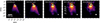 |
Fig. 5 MIRI-MRS images of continuum emission from cubes centered on 6.3, 13.8, 19.6, 22.4, and 26.4 μm, from left to right. The images were generated by integrating cubes over 0.6 μm around the central wavelength. The cubes were PSF-subtracted before the imaging. The white star marks the position of the protostar in the mid-IR. |
3.1.4 Extended continuum emission maps
One of the most striking features we found in the BHR71-IRS1 MIRI-MRS observations after we removed the protostellar PSF is the clear presence of the extended continuum emission (see Fig. 1, bottom right). This emission could originate from heated dust or photons released by accretion, it might be scattered off dust, or a combination of the two.
Fig. 5 shows the continuum maps at different wavelengths after the PSF subtraction. The maps were created by integrating 0.6 μm centered at 6.3, 13.8, 19.6, 22.4, and 26.5 μm. Two clear extended-emission components are detected: the first component, along the jet, is clumped into a series of bullets that is most clearly seen at longer wavelengths. The clumps are well aligned with positions B1-B4 seen in the gas lines of the jet. The second component is seen along the cavity wall and is asymmetric, brighter on the western side, similarly to the CO2 emission, also in spatial extent (Fig. 4, middle left). CO2 and the corresponding continuum component both match the width of the low-excitation H2 lines (Fig. 3, right). Close to the source, the western side appears to be brighter in continuum than the eastern side, similarly to what is shown in the ro-vibrational CO map (Fig. 4, left).
At longer wavelengths, this component persists, suggesting that it is not only scattered light, but also thermal emission from warm dust. The component is also seen to fill the outflow cavity, and we therefore infer that this emission is not only warm dust shock- or UV-heated at the cavity walls, but also wind-entrained dust. The continuum emission along the jet is co-spatial with the bullets. Residual emission also appears to be close to the source and is not subtracted by the PSF removal. It might arise from a cold, extended envelope.
3.2 Spectra, line fluxes, and line ratios
From the regions shown in Fig. 1 (top right), we extracted spectra using circular apertures with a diameter of 1″.0 at several positions: four bright ionized knots (bullets B1-B4), one bullet at the western side of the outflow cavity (CR1), and another farther along the outflow (O5), where no atomic jet is detected. The regions are presented in Fig. 1 (top right), and their coordinates are listed in Table E.2. The resulting spectra are presented in Fig. E.3 (for spectra extracted on-source, see van Gelder et al. 2024).
To obtain the total flux of the emission lines, we fit a linear function to the local continuum in the line-free channels to the 0.24 μm region, which is broad enough for a local continuum fit centered on the line rest wavelength, and a Gaussian profile to the emission line. From the area below the Gaussian divided by the aperture area, we obtained the line intensity. Since the region size was selected to fill the entire region, we assumed that no filling factor was required. The Gaussian centroid provides information about the radial velocity offset of the line. In the case of a non-detection, we obtained the upper limit by using three times the RMS derived from a line-free part of the spectrum, multiplied by the empirical FWHM of MIRI based on in-flight calibration data. This ranges from 75 to 294 km s−1 for channels 1 to 4, respectively (Argyriou et al. 2023). In several cases, the emission lines are blended with the superimposed molecular emission (e.g., CO and H2O) originating from the disk and/or outflow. There, we first fit a slab model to the continuum-subtracted spectra and subtracted it from the data before we fit the remaining emission lines (for details of the slab model fit, see van Gelder et al. (2024). The fluxes were corrected for extinction using H2 derived values (see Appendix C). The measured line intensities and velocity offsets are reported in Table E.3.
The variations in the physical conditions are reflected in the extinction-corrected line ratios for the selected species. In Fig. 6 we compare the line ratios that are sensitive to the gas temperature for species with similar ionization potentials (left) and for the ionization fraction for species at comparable upper energy levels (right). In addition, Fig. E.1 presents the peak brightness as a function of distance from the protostar for selected lines and the continuum at 19.6 μm.
Fig. 6 (left) shows that the line ratio of two [Fe II] lines at 17.9 μm (Eup = 3496 K) to 25.99 μm (Eup = 554 K) is constant for bullets B1 to B3 and then decreases by a factor of 5 at the position of B4. For two transitions of [Ni II] at 10.68 μm (Eup = 13 424 K) and 6.63 μm (Eup = 2168 K), the ratio decreases from B1 to B2, then remains approximately constant from B2 to B3, and further decreases in B4. The [Co II] 14.56 μm (Eup = 5797 K) to [Co II] 10.52 μm (Eup = 1368 K) ratio initially increases from B1 to B3 and then decreases in B4. Overall, this shows that the gas temperature remains roughly constant from B1 to B3, and it then drops significantly for B4. This is also supported by a non-LTE model, which for two ratios of [Fe II], 25.9 μm to 17.9 μm and 17.9 μm to 5.3 μm, shows a gradual increase in the electron temperature from B1 to B3 and a sharp decrease for B4 (Fig. D.3)
Fig. 6 (right) shows that three tracers of the ionization fraction, [Fe II] (7.9eV) to [Fe I], [Cl II] (13 eV) to [Cl I], and [Ne III (41 eV) to [Ne II] (21.6 eV) all increase from B1 to B3 and then decrease at B4. The exception is the line ratio of [Ne II] (21.6 eV) to [Ar II] (15.8 eV), which decreases from B1 to B3. We interpret this as still being consistent with the pattern of increasing ionization conditions from B1 to B3, since the decrease in [Ne II] to [Ar II] is likely an effect of [Ne II] being further ionized to [Ne III].
We combined these pieces of information from the line ratios together and found that at the inner bullets (B1-B3), the gas experiences a high temperature: collisional excitation produces strong [Ne II], [Ar II], and high Eup [Fe II] emission. At B4, the conditions change abruptly and result in less excited gas and weaker emission of ions with respect to neutral species. The refractory variations along the jet are consistent with changes in the shock efficiency that disrupt grains.
From the line brightness profiles shown in Fig. E.1, we also infer that closer to the protostar, that is, in the inner 300 au region, [Fe I] and [S I] are brightest, which suggests that the gas is launched in a neutral state, likely due to the high-density conditions, and is only ionized further at the internal working surface bullets. This increase in density is also supported by the electron density found from the [Fe II] line ratios in Fig. D.3.
With the limited spectral resolution of MIRI, a detailed analysis of the kinematics is challenging. However, by fitting Gaussian profiles to the emission lines, we obtained information on the average velocity in the region from which the spectra were extracted. In Figure 7, we present the values of the centroid positions converted into the line velocity with respect to the rest wavelength of the transition measured at selected apertures B1-B4 along the jet for selected atomic, ionic, and molecular emission lines as a function of distance from the protostar. All values were corrected for inclination, set in reference to the LSR, and corrected for cloud velocity (vLSR = -4.7 km s−1 Kristensen et al. 2012). For CO, we fit multiple emission lines from the ro-vibrational spectra, masking those contaminated by H2 lines, for a total of 14 lines in 4.9 to 5.1 μm range, thereby improving the accuracy of this measurement. In Fig. 8, we show for each bullet the H2 rotational transition velocity as a function of the upper energy levels.
We identified two key features in the measured velocities. First, within a single aperture, the centroid velocity of the H2 emission lines increases with the upper energy level of the transition (Fig. 8). The second observed trend is an increase in velocity up to bullet B3, followed by a decrease in position B4 for [Ne II] and [Fe II], while [S I] remains constant (Fig. 7). The average offset of CO lines shows a different pattern. The velocities oscillate between -240 km s−1 and -180 km s−1 in inclination-corrected radial velocities, and the trend of the oscillation is opposite to the trend seen in H2 . This can be also related to Fig. 6, where B3 shows peak ionization, and E.2, where [Ne II]/[Fe II] shows the highest ratio at this spot. All this indicates strong ionization.
The velocities of H2 seem to oscillate from B1-B4, but show an overall increasing trend. The inclination is based on the overall source properties (Yang et al. 2020) and should therefore be treated as the average. The jet wiggling can affect the relative velocities. However, the absolute inclination uncertainty applies similarly to all lines and is therefore not relevant here.
Taking the average flow velocity based on [Fe II] 5.34 μm at all bullets, we can estimate the dynamical scale of the outflow. For the vmean = -222 km s−1 and distance to B4 of 1483 au, the averaged timescale of the jet is 32±1 years. On-source H2O, CO2 , and SiO ro-vibrational lines are also detected with lower velocities of -42, -10, and -23 km s−1, respectively, as reported in van Gelder et al. (2024).
 |
Fig. 6 Line ratios of selected species at positions B1-B4 plotted as a function of the deprojected distance from the source. Left : ratios of the same species sensitive to the gas temperature: [Co II] 14.5 μm to [Co II] 10.5μm (orange), [Fe II] 17.9 μm to [Fe II] 25.9 μm (blue), and [Ni II] 10.6 μm to [Ni II] 6.6 μm (green). Right : ratios sensitive to the ionization fraction: [Fe II] 25.9μm to [Fe I] 24.0 μm (gray), [Ne II 12.8 μm to [Ar II] μm 6.9 μm (brown), [Cl II] 11.3 μm to [Cl I] 14.4 μm. (pink), and [Ne III] 15.55 μm to [Ne II] 12.8 μm (purple). |
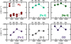 |
Fig. 7 MIRI-MRS centroid velocity with respect to the vLSR of the protostar and corrected for source inclination for selected emission lines. |
 |
Fig. 8 MIRI-MRS centroid velocity of H2 rotational transitions with respect to the vLSR of the protostar and corrected for the source inclination as a function of Eup. The color shows different positions along the jet (see Fig. 1, top right) |
4 Analysis
4.1 Characterization of the extended dust emission
To characterize the extended dust emission from system BHR71-IRS1, we extracted the spectra as described in Section 3.2. We used the PSF-subtracted cubes to minimize the contribution of the central source to the extended continuum (Appendix A). We modeled the dust continuum for each aperture by assuming a dusty emitting region extincted by intervening dust. We flagged line channels with the fast automatic baseline fabc algorithm in pybaselines (σscale = 5 channels, Nstd = 5, Erb 2025). Then, we proceeded with uncertainty-weighted least-squares fitting with lmfit (Newville et al. 2025). We assumed warm and cold emitting regions at temperatures Tw and Tc, with angular areas Ωw and Ωc. Both regions had dust with an absorption  and isotropic single-scattering
  opacities (in cm2 g−1),
![Mathematical equation: F^{\rm dust}_{\nu} = \frac{\kappa_\nu^{\rm abs} [\Omega_{\rm c}B_\nu(T_{\rm c}) + \Omega_{\rm w}B_\nu(T_{\rm w})] + 2\kappa_\nu^{\rm sca} F^{\rm ps}_\nu}{\kappa_\nu^{\rm abs} + \kappa_\nu^{\rm sca}},](/articles/aa/full_html/2026/06/aa58711-25/aa58711-25-eq3.png) (1)
(1)
where the scattered stellar radiation  is a blackbody, subtending an angular size Ωps from the perspective of the emitting region,
  . The dust emission
  was then screened by a dust layer with surface density Σ (g cm−2), with an optical depth
  , leading to an observed flux density of
  . We used the KP5 dust model for our opacities (Pontoppidan et al. 2024). In the 5-27 μm range, scattering cannot be ignored, and optically thin dust cannot necessarily be assumed. We assumed isotropic scattering, as including anisotropic scattering is a constant factor that is absorbed in Ωps from an unknown inclination angle. The surface density Σ allowed us to estimate the mass along the line of sight that caused the extinction. It does not distinguish between ISM dust in the line of sight, the envelope, or possible dust in the cavity. However, due to the large variations in AV on the spatial scales of MIRI MRS, we considered the envelope mass to be the dominant contributor to Σ. We reserve a detailed dust modeling (composition, size distribution, and porosity) for future work. The fit for the B1 position is presented in Fig. 9 and is shown for the remaining positions in Fig. B.1.
The measured dust properties, that is, temperature, IR flux, and surface density of the extincting dust, are summarized in Fig. 10 and Table E.1. In the top panel, we show the temperature of the warm and cold dust components as a function of distance from the protostar. The temperature of the cold component is constant with distance, at approximately 80 K. In contrast, the warm component has a clearly decreasing trend from 406 ± 6 K at B1 to 201 ± 42 at B4. In the bottom panel, we plot fluxes at 13 μm and 22 μm, where the emission is dominated by the warm and cold components, respectively. Both decrease with distance from the protostar, but the brightness of the cold component decreases more sharply. This is consistent with the powerlaw decrease in the envelope density modeled for this source (ρ ~ r−1.; Kristensen et al. 2012). Together with the temperature of the cold component (similar to Tbol = 66 K), this might indicate that at least part of the flux might stem from the extended envelope and not from the jet itself.
We next investigated whether the continuum emission observed in the jet and at the outflow cavity wall might be dominated by scattering. Based on the brightness profile as a function of wavelength, we conclude that it is dominated by thermal emission and not by scattering. Fig. 5 shows the evolution of the dust emission as a function of wavelength. Bullets only appear as continuum emission components above 13 μm. As shown by Duchêne et al. (2024), large grains show a flat scattering opacity at mid-IR wavelengths even up to 20 μm (see also Kataoka et al. 2014). Therefore, the bullets would have to show a similar brightness across wavelengths. On the other hand, in the case of emission at the outflow cavity walls, where emission persists across wavelengths, the scattering can be a factor. The fitting presented here likely underestimates the scattering since we implemented large grains in the fit. Large grains (~10 μm) at the outflow cavity walls of BHR71 have been suggested before by polarization studies (Hull et al. 2020). In summary, for the cavity walls, the scattering might be a significant factor and might cause us to overestimate the temperature of the grains in the envelope. However, scattering is unlikely to contribute significantly to the emission in the jet bullets.
The warm-dust component cools from 406 to 201 K on a scale of 1000 au. If the temperature decreased linearly, the dust would have a temperature above 450 K at the launch point. This estimate does not include additional heating. In the absence of a heat source, dust would cool on timescales of seconds to days (Draine & Anderson 1985), and therefore, the presence of warm dust at such distances would require additional heating. Based on the average velocity of the [Fe II] 5.34 μm (see Section 3.2), the travel time to B4 from the source would be 32±1 years, and it would be 23±1 years from B1 to B4.
The surface density of the dust causing the extinction decreases with distance from the protostar. A decrease is consistent with the lower density of the envelope with radius, comparable with the model (Table C.1 in Kristensen et al. 2012). The surface density can be directly converted into extinction, yielding values of 32, 15, 12, and 7 mag for the bullets B1-B4. The values are systematically lower than those measured with H2.
In summary, we identified warm (200-400 K) and cold (80 K) emitting components of the dust in the BHR71-IRS1 wind in the collimated and wide-angle components. The majority of the dust is expected to be launched directly by the wind, but detailed radiative transfer modeling is necessary to identify its physical origin.
 |
Fig. 9 Fits to the SED at position B1. The extracted SED was smoothed with a Gaussian kernel. The dashed lines indicate the scattered, warm, and cold dust components, shown in blue, orange, and green, respectively. The solid red line shows the sum of the three blackbodies. The dashed purple line shows the sum of the blackbody temperatures extincted with the KP5 extinction curve. |
 |
Fig. 10 Top : fitted dust temperatures to warm and cold blackbody components for the SEDs in Figs. 9 and B.1. Middle : IR fluxes at 13 and 22 μm as a function of distance from the protostar. The modeled envelope density as a function of radius is shown as the dashed red line (Kristensen et al. 2012). Bottom : surface density of the extincting dust as a function of distance from the protostar. The dashed red line same as in the middle panel. |
 |
Fig. 11 Top : properties of the shock along the jet. Positions B1-B4 are indicated in Fig. 1, and the shock modeling results are summarized in Table D.1. The range of values stems from the density estimate based on S and Cl. Bottom : Fe and Ni abundance at the B1-B4 shock positions based on the shock model as measured in Appendix D. |
4.2 Shock models: Velocity, density, and elemental abundances
We compared the extracted line intensities with the shock model of HM89. The procedure is detailed in Appendix D. The results are presented in Table D.1 and are illustrated in Fig. 11 with ranges coming from the differences between the [S I] and [Cl I] estimates. The shock velocity decreases from above 70 km s−1 to 35 km s−1 from bullet B1 to B4, with a constant shock velocity of 60 between bullets B2 and B3. The pre-shock density across the jet also decreases with distance from the protostar from above 105 cm−3 to 4 × 104 cm−3, except for bullet B4, which shows a small increase in the pre-shock density compared to a position closer to the protostar.
We then used the derived conditions in the shock models to derive the jet mass ejection rate and also to assess the elemental depletion. The density of the pre-shock gas decreases with distance from the protostar, while at the same time, the (radial) velocity of the flow increases with distance, which results in a relatively constant mass-loss rate of 1.7-3.4 × 10⁻⁷ M⊙ yr−1. When the density estimate from [Cl I] is used instead, a range of 1.5-23.3 × 10⁻⁷ M⊙ yr−1 is measured.
4.3 Shock models: Elemental abundances
Based on the estimated shock properties, we assessed the depletion of different species relative to solar values. The pre-shock density and shock velocity provide an expected line intensity for a specific tracer. The difference between the measured intensity and the value predicted by the model is assumed to be due to depletion of the species in the gas phase, as indicated by a ratio of species to atomic sulphur, which is expected to be volatile. It can therefore provide a reference of solar values as an undepleted species. We also assumed that sulphur was predominantly in atomic and not in molecular form. Higher values for Cl, especially above 1, can be attributed to the fact that some of the chlorine might be in neutral form, given its relatively high 23.81 eV ionization potential, or that Cl is less refractory than Fe, Ni, and Co. Co depletion would be of great interest, but the transitions of [Co II] are not included in HM89. Overall, the significant depletion of refractories relative to solar values suggests that even under strong shocks, dust survives. This agrees with models for C-type and J-type shocks (Guillet et al. 2009; Gusdorf et al. 2008). If the dust we observe is lifted from the disk, its presence also means that it comes from beyond the dust-sublimation zone.
5 Discussion
5.1 Extended thermal dust emission
While there is evidence of dust in protostellar winds through their refractory abundances (e.g., Podio et al. 2006; Dionatos et al. 2009); MIRI imager scattered-light observations (Duchêne et al. 2024), ALMA continuum observations of the low-emissivity suggestive of large grains possibly launched by the wind (Sabatini et al. 2024, 2025), and polarization studies indicating grain growth at the outflow cavity walls (Le Gouellec et al. 2019; Hull et al. 2020), the MIRI-MRS mode observations so far revealed extended dust continuum emission close to the source only around two protostars: HH211 (Caratti o Garatti et al. 2024) and BHR71-IrS1 (this work). The presence of dust in the high-velocity wind (jet), spatially separated from the wide-angle wind component, and the outflow cavity walls, provides the strongest evidence so far that the grains are lifted from the disk. It remains an open question whether these grains might then fall back onto the outer disk and envelope and contribute to the reservoir of calcium-aluminium inclusions (CAI) (Shu et al. 2001). In this section, we discuss the properties of the observed dust and possible scenarios for its origin.
5.1.1 Origin of the extended continuum emission
We detected two different spatially extended components: conelike continuum emission along the outflow cavity walls that decreased with distance from the protostar, slightly asymmetric with a brighter western side, and emission in the jet beam, co-spatial with the ionized high-velocity gas bullets.
The cone-like emission can either be interpreted as dust that launched with the wind or was already present at the outflow cavity wall. These scenarios were discussed in detail by Sabatini et al. (2025), who found a dust opacity spectral index ≤1.3, which they interpreted as evidence of millimeter-sized grains. However, low spectral indices can also be caused by large temperature variations due to interior heating (Ysard et al. 2019). Further, large grains can more easily be destroyed by radiation than small grains (Hoang 2019), so an investigation combining MIRI spectroscopy with ALMA continuum observations is needed. Sabatini et al. (2025) provided strong arguments for the scenario in which the dust is launched in the wind. They rejected the scenario of grains already present in the envelope because millimeter-size grains were detected, which are difficult to form in a low-density outer envelope (Silsbee et al. 2022; Lombart et al. 2026). In the case of BHR71-IRS1, Hull et al. (2020) estimated the size of the largest grains in the outflow cavity walls to be 10 μm at least.
For the dust detected in the collimated jet, we favor the scenario of dust that is directly lifted with the wind with respect to the envelope dust entrained and compressed in the jet. This latter hypothesis is disfavored for several reasons discussed below. We detected higher dust continuum emission at the exact positions of the ionized emission from the internal working surfaces of the jet (Figs. 1, 5, and E.1). At the knot positions, the continuum emission increases with respect to the background emission from the outflow cavity walls, so it is a distinct jet feature and not envelope material. In addition, if the dust were coming from the entrained envelope, it should be more strongly correlated with the H2 emission or the cold CO gas (see Fig. 3), which are more likely tracers of the entrained gas than the jet.
Although the jet is precessing, it is not likely that the dust in knots is entrained material from the envelope. The dust emission is seen across the bullets from 300 up to 1500 au. Dust emission is seen consistently throughout the jet and not just at the front of the jet. If this were shocked and compressed entrained dust, the limited refilling of the cavity might explain the presence of the dust at the furthermost bullet, but then, little dust would remain to be shocked in bullets closer to the source, and if anything, the dust emission would be fainter from B4 to B1, while we see an opposite trend.
Modeling work in recent years provided substantial evidence for the feasibility of transport and launching of grains in the protostellar wind (e.g., Wong et al. 2016; Liffman et al. 2020; Vinkovic & Cemeljic 2020; Booth & Clarke 2021). Giacalone et al. (2019) provided a model for dust launching in the magnetohydrodynamic (MHD) disk winds and related the amax, maximum size of the launched grains to the accretion rate, stellar mass, gas temperature in the launching zone, and the launching radius. For fiducial parameters adopted for T Tauri disks (Ṁacc ∼ 10−8, and M* ∼ 1 M⊙), they obtained amax = 0.35 μm. The mass-loss rate of our source is higher by an order of magnitude and that the stellar mass is lower by a factor of two, so that this will provide a size of 7 μm at the same launch radius and disk temperature. Bhandare et al. (2024) self-consistently explored dust transport from sub-au scales with the hydrodynamics code PLUTO, showing that grains can be efficiently redistributed across the disk by means of outflows for grains up to 100 μm, while Tsukamoto et al. (2021) showed that even millimeter-size grains can be lifted by the winds.
Recent direct observations of crystallization occurring in the disk during outbursts by Lee et al. (2026) showed that seeds of processed grains can be formed in the inner disk. The launch of them in the wind and transport to the outer disk explains their presence in the outer Solar System. That work also predicted a variable dust composition depending on the launch radius. Detailed studies of the launched dust composition will be able to provide more information on this process.
5.1.2 Dust survival and launch radius
Because dust sublimates at small radii, the inner disk within the dust-sublimation radius is expected to be essentially dust free; therefore, any dust observed in the wind must originate at disk radii larger than the sublimation radius. For BHR71-IRS1 (Lbol ≈ 10 L⊙), thia radius is ∼0.2 au under standard assumptions for the dust sublimation temperature (Tsub ≈ 1500 K; Dullemond & Monnier 2010). The detection of dust in the ejected gas thus favors a disk-wind origin (which launches from larger radii) over a classical X-wind. However, under certain conditions, X-wind models can still accommodate dust launching if the launch point shifts outward during an accretion outburst (Shu et al. 1997). Therefore, the presence of dust does not conclusively distinguish between these scenarios; instead, it indicates either a launch from radii outside the sublimation zone or a temporary outward shift of the launch radius.
Accretion outbursts can increase the dust fraction in launched winds. MHD models predict that dust-to-gas ratios in winds can rise during outbursts (Kadam et al. 2025), so a recent outburst (on the flow dynamical timescale, ≲50 yr) might explain the dust. Outbursts also raise the IR luminosity and the grain alignment efficiency, and in turn, they increase the probability that grains are disrupted by their rotation (Hoang 2019). However, according to simulations and synthetic observations, this increase in IR luminosity does not destroy all grains on typical dynamical timescales of 10-100 yr, except for the largest sizes and least cohesive grains (Hull et al. 2020; Le Gouellec et al. 2023; Giang et al. 2025). This leaves the possibility of the presence and survival of small and compact grains in irradiated outflow cavities. This scenario might account for the apparent truncation of the atomic jet beyond knot B4, which might mark the onset of recent outburst activity.
5.1.3 Dust temperature and heating source
The observed dust temperature cannot be assumed to be simply the temperature at the launch point because grains cool very rapidly: for example, a 0.1 μm silicate grain at 100 K radiatively cools to ∼10 K on a timescale of seconds (Draine & Anderson 1985). Thus, the dust must be continuously heated by a local or external source. Maintainenance of grain temperatures ≳100 K by UV radiation alone requires a very strong field (G0 ≳ 105) (e.g., Hocuk et al. 2017). The detection of prompt OH emission, a tracer of H2O photodissociation, indicates an internal UV field in the jet (Tabone et al. 2021). Lehmann et al. (2020) used the shock model to predict 102 G0 for shock velocities of 60-75 km s−1, which were inferred in bullets B1-B3, and of 101 G0 for bullet B4. The lack of a clear correlation between OH flux, shock velocity, and dust temperature suggests that shock-generated UV is not the dominant dust heater; additional heating from protostellar accretion luminosity is therefore required to explain the warm dust. However, typical models of dust temperatures in the envelope do not predict sustained dust temperatures of several hundred K at 1000 au from the protostar (Nazari et al. 2024). While low-velocity shocks and C-type shocks cannot heat the dust above 100 K (Miura et al. 2017; Draine et al. 1983), the J-type shock model presented in Hollenbach & McKee (1979) predicts that higher temperatures can be reached by J-type shocks (∼300 K for vs = 80 km s−1 and n0=105 cm−3). The specific dust temperature in shocks is determined by the grain and shock properties. Qualitatively, the grain temperature increases with shock velocity and pre-shock density, and it is higher for smaller grains (HM89). We note that the trend of the temperature of the warm component (Fig. 10, left) is similar to that of the shock velocity (Fig. D.1, top right), which is consistent with heating of the dust grain to higher temperatures in a faster shock. The exact contributions of photospheric, accretion, and shock heating of the grains would require radiative transfer modeling.
5.1.4 Comparison with chemical tracers
Other species provide complementary constraints. SiO is seen in absorption toward the protostar at an offset of ∼40 kms−1 (van Gelder et al. 2024), which is consistent with part of the SiO gas originating from regions at or interior to the sublimation zone, where silicon is liberated from grains (Gusdorf et al. 2008). ALMA does not detect extremely high-velocity SiO in this source (Gavino et al. 2024), which is consistent with gas mass-loss inferred from atomic tracers of 10−7 M⊙ yr−1, which is too low for formation of molecules (Tabone et al. 2020).
Comparisons with spectrally resolved far-IR observations (e.g., Herschel/HIFI) suggest that the low-Eup H2O gas identified in these data likely originated in regions more closely associated with the extended H2 emission than with the high-velocity ionic jet (Kristensen et al. 2012; Mottram et al. 2014). Faintly detected cold H2O rotational transitions in the MIRI data likely trace the same component as Herschel, but the signal-to-noise of the H2O does not allow us to estimate the velocity. CO and CO2 show a distinct spatial behavior: CO2 coincides with warm dust at the cavity walls, whereas CO is stronger where CO2 is weak near the source. This might indicate that the shocks on the western cavity wall related to jet wiggling are stronger.
5.2 Difference between Class 0 and Class I outflows and jets
We compared the BHR71-IRS1 jet to other spatially resolved jets from Class 0 and Class I protostars, leveraging the unprecedented mid-IR resolution of the JWST. Earlier facilities (e.g., Spitzer) lacked the spatial resolution to separate wind layers close to the source (Lahuis et al. 2010), but recent JWST studies have revealed diverse disk-wind signatures in Class I systems (Tychoniec et al. 2024; Delabrosse et al. 2024; Harsono et al. 2023; Assani et al. 2024).
In Class I sources, the wind typically appears to broaden at lower upper-level energies, which is consistent with a layered outflow structure, whereas in BHR71-IRS1, the outflow boundary remains sharp, resembling that of HH46 (Nisini et al. 2024). Even high-excitation H2 lines do not show a narrow, jet-like core, as seen in some other objects, where high-J H2 traces a molecular cocoon around the jet (Caratti o Garatti et al. 2024; Navarro et al. 2025; van Dishoeck et al. 2025; Francis et al. 2026). The relative lack of molecular emission in the collimated jet, as evidenced by ALMA, might reflect evolutionary differences or distinct shock conditions (Nisini et al. 2015).
Excitation diagnostics highlight clear contrasts with the Class I source HH46. The line ratios indicate higher excitation in HH46: iron lines imply warmer collimated gas, [Ne II]/[S I] is higher by some orders of magnitude in HH46 than in BHR71-IRS1, and [Ne III] is detected in HH46, while [Fe I] is not. These differences indicate a more highly ionized lower-density jet in HH46 than the denser, more weakly ionized BHR71-IRS1. By contrast, the refractory ratios with a similar excitation, for example, [Ni II] 6.64 μm/[Co II] 10.52 μm, are similar for BHR71-IRS1 and HH46 (within a factor of two). This suggests that despite differences in excitation regimes, the relative abundances of these refractory species are comparable and not strongly affected by evolutionary stage.
The strong [Ne II] 12.8 μm emission along the BHR71-IRS1 jet concentrated in several bullets supports the presence of J-type shocks in which H2 can be dissociated and later reformed on grains (HM89). In contrast to very young Class 0 sources such as HH211, where H2 is clearly detected in the high-velocity collimated wind (Caratti o Garatti et al. 2024), H2 in BHR71-IRS1 appears to be more extended and likely traces jet-cavity interactions and shocked cavity walls. H2 centroids are also systematically slower than the ionized jet velocities, which is consistent with an origin in post-shock or entrained gas and not in the primary high-velocity jet.
Overall, BHR71-IRS1 exhibits characteristics of a late-stage Class 0 source: its H2 morphology resembles that of Class 0 systems (compact molecular structures near the jet and cavity), while its atomic and ionic emission indicates still lower excitation than most Class I jets.
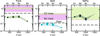 |
Fig. 12 Left : Fe to S elemental ratio compared with the solar abundance (dashed gray line) and non-carbonaceous (NC) and carbonaceous (CC) iron meteorites (green and purple shaded areas, respectively; Grewal et al. 2024). Middle : Ni to S elemental ratio. Right : Ni to Fe elemental ratio. |
5.3 Refractories and planetary building blocks
Jets sample material from the innermost disk. They can thus carry information about the composition of solids that may later contribute to planet formation. Refractory elements such as Ni, Co, and Fe have similar condensation temperatures and ionization potentials, making their relative abundances useful probes of dust processing and elemental depletion in the inner disk (Wood et al. 2019; Konstantopoulou et al. 2022). Figure 12 compares the refractory ratios measured in the jet with Solar and meteoritic (non-carbonaceous and carbonaceous iron meteorites) values (Grewal et al. 2024). We also note that the abundances of primitive chondritic meteorites are usually similar to the solar values (Lodders 2021). Although Fe and Ni, the two refractories for which we can establish abundances based on the shock models, show an overall depletion relative to their solar abundances, they are compared to S, treated here as a volatile reference (Fig. 12, left and center). However, the Ni/S ratio is closer to the solar value, especially at positions B1-B3. For Fe and Ni, this means that the values are also much lower than those of iron meteorites.
The Ni/Fe ratio appears to be higher than the solar value and within the range of iron meteorites. The ratio is also similar to the Ikeya-Seki comet (0.08; Preston 1967), and at the same time, it is much lower than that of Oort cloud comets (0.87; Manfroid et al. 2021) and pre-solar SiC (~5.5; Marhas et al. 2008). In comets, the ratio is explained by the lower sublimation temperature of the Ni-bearing compounds than the Fe-bearing ones (Manfroid et al. 2021) (see also the discussion in Samland et al. 2025). Perhaps this is the reason for the lower Ni depletion relative to solar values and the Ni/Fe excess in the BHR71-IRS1 jet, especially if it is released from NiS.
However, the interpretation of the abundance patterns requires caution. The apparent depletion of refractories relative to volatiles might reflect the retention of refractory material in large grains that survive the launch and incomplete grain destruction in the jet shocks. Our detection of warm dust in the jet supports the view that grains are not fully destroyed, implying that measured gas-phase refractories trace only a fraction of the total refractory budget. If jet measurements reliably trace the inner-disk composition, they can inform models of early planetesimal formation and the chemical dichotomy observed in the Solar System. However, it is difficult to assess the size distribution of ejected grains with the current data.
More systematic surveys of refractory abundances in jets across evolutionary stages are needed to establish whether jets can provide robust population-level constraints on the initial composition of planet-forming solids. The inclusion of cobalt in shock models, now readily detected in jets, would open a new avenue for studying the relative abundances of refractories.
6 Summary
We detected and resolved for the first time the ionized jet at the center of the outflow from the BHR71-IRS1 protostar, along with the warm dust, with JWST-MIRI MRS. The main results are summarized below:
The jet is bright in refractory gas, with species of ionized and neutral fine structure lines of Fe, Ni, Cl, and Co. The collimated emission is concentrated into four knots. In addition, molecular lines of OH, CO, H2O, and CO2 are detected in the outflow;
The extended thermal dust continuum is fitted toward each bullet with three components: scattered light from the protostar, and two thermal components: warm (200-400 K) and cold (∼80 K). The cold component is present throughout the envelope, with a temperature that is nearly constant; the temperature of the warm component decreases with distance. The presence of the warm component both on and off-axis of the jet (in the wide-angle wind) can be interpreted as dust entrained in the wind as well as in the collimated jet, while the origin of the cold component is more ambiguous, with possible contribution from the entrained envelope;
The jet is surrounded by H2 molecular gas, which is radially extended and peaks corresponding to the ionized jet. The H2 flow extends beyond the radial distance of the jet;
Using [Ne II], [S I], and [Cl I], we estimated the shock conditions. The shock velocity decreases with distance from the protostar from 70 km s−1 to 38 km s−1. The shock density drops from above 105 to 3-4 × 104 cm−3 with distance from the protostar;
We used the shock models to estimate the abundance of refractory species relative to volatile sulfur. We found that iron and nickel are both depleted relative to solar abundances. Together with the dust detected in the jet beam, this provides strong evidence of dust launching in the jet.
The protostellar jet BHR71-IRS1 reveals bright refractory lines and dust thermal emission. Further studies of the dust properties and the abundance of refractory elements might help us to elucidate the composition of planetary building blocks at the earliest stages of planet formation.
Acknowledgements
We thank the referee for careful evaluation of the manuscript and comments that improved the clarity of the presented results. This work is based on observations made with the NASA/ESA/CSA James Webb Space Telescope. The data were obtained from the Mikulski Archive for Space Telescopes at the Space Telescope Science Institute, which is operated by the Association of Universities for Research in Astronomy, Inc., under NASA contract NAS 5-03127 for JWST. These observations are associated with program #1290 https://doi.org/10.17909/7eh1-8f25. The following National and International Funding Agencies funded and supported the MIRI development: NASA; ESA; Belgian Science Policy Office (BELSPO); Centre Nationale d’Études Spatiales (CNES); Danish National Space Centre; Deutsches Zentrum fur Luftund Raumfahrt (DLR); Enterprise Ireland; Ministerio De Economiá y Competividad; The Netherlands Research School for Astronomy (NOVA); The Netherlands Organisation for Scientific Research (NWO); Science and Technology Facilities Council; Swiss Space Office; Swedish National Space Agency; and UK Space Agency. This paper makes use of the following ALMA data: ADS/JAO.ALMA#2019.1.00261.L ALMA is a partnership of ESO (representing its member states), NSF (USA) and NINS (Japan), together with NRC (Canada), NSTC and ASIAA (Taiwan), and KASI (Republic of Korea), in cooperation with the Republic of Chile. The Joint ALMA Observatory is operated by ESO, AUI/NRAO, and NAOJ. The National Radio Astronomy Observatory is a facility of the National Science Foundation operated under cooperative agreement by Associated Universities, Inc. This research has made use of NASA’s Astrophysics Data System Bibliographic Services. MvG, LF, EvD, YC, KS, acknowledge support from ERC Advanced grant 101019751 MOLDISK, TOP-1 grant 614.001.751 from the Dutch Research Council (NWO), The Netherlands Research School for Astronomy (NOVA), the Danish National Research Foundation through the Center of Excellence “InterCat” (DNRF150), and DFG-grant 325594231, FOR 2634/2. T.P.R. acknowledges support from ERC grant 743029 EASY. H.B. acknowledges support from the Deutsche Forschungsgemeinschaft in the Collaborative Research Center (SFB 881) “The Milky Way System” (subproject B1). A.C.G. acknowledges support from PRIN-MUR 2022 20228JPA3A “The path to star and planet formation in the JWST era (PATH)” funded by NextGeneration EU and by INAF-GoG 2022 “NIR-dark Accretion Outbursts in Massive Young stellar objects (NAOMY)” and Large Gran INAF-2024 “Spectral Key features of Young stellar objects: Wind-Accretion LinKs Explored in the infraRed (SKYWALKER)”. KJ acknowledges the support from the Swedish National Space Agency. P.N. acknowledges support from the ESO Fellowship and IAU Gruber Foundation Fellowship programs. JMV acknowledges support from the Academy of Finland grant No. 348342. D.H. is supported by the Ministry of Education of Taiwan (Center for Informatics and Computation in Astronomy grant and grant number 110J0353I9) and the National Science and Technology Council, Taiwan (Grant NSTC111-2112-M-007-014-MY3, NSTC113-2639-M-A49-002-ASP, and NSTC113-2112-M-007-027). Y.-L.Y. acknowledges support from Grant-in-Aid from the Ministry of Education, Culture, Sports, Science, and Technology of Japan (20H05844 and 25H00676). The project was supported by RIKEN Incentive Research Project (Emergence of pre-biotic extraterrestrial world: Using machine-learning techniques to uncover the link of organic matter at the dawn of planetary systems). This research made use of NumPy (Harris et al. 2020); scipy (Virtanen et al. 2020), Astropy, a community-developed core Python package for Astronomy (Astropy Collaboration 2022); Matplotlib (Hunter 2007), lmfit (Newville et al. 2025), stpsf (Perrin et al. 2025), jwst (Bushouse et al. 2023), pandas (pandas development team 2020) . This research made use of Photutils, an Astropy package for detection and photometry of astronomical sources (Bradley et al. 2025). We utilized GitHub CoPilot to assist in writing parts of the code for the analysis, accessed through the Visual Studio Code extension GitHub Copilot Chat. We used Grammarly for grammar and spelling corrections.
References
- Agra-Amboage, V., Dougados, C., Cabrit, S., & Reunanen, J. 2011, A&A, 532, A59 [NASA ADS] [CrossRef] [EDP Sciences] [Google Scholar]
- Allen, C. W. 1973, Astrophysical quantities [Google Scholar]
- Anglada, G., López, R., Estalella, R., et al. 2007, AJ, 133, 2799 [Google Scholar]
- Argyriou, I., Glasse, A., Law, D. R., et al. 2023, A&A, 675, A111 [NASA ADS] [CrossRef] [EDP Sciences] [Google Scholar]
- Assani, K. D., Harsono, D., Ramsey, J. P., et al. 2024, A&A, 688, A26 [NASA ADS] [CrossRef] [EDP Sciences] [Google Scholar]
- Astropy Collaboration (Price-Whelan, A. M., et al.) 2022, ApJ, 935, 167 [NASA ADS] [CrossRef] [Google Scholar]
- Barsony, M., Wolf-Chase, G. A., Ciardi, D. R., & O’Linger, J. 2010, ApJ, 720, 64 [NASA ADS] [CrossRef] [Google Scholar]
- Benedettini, M., Gusdorf, A., Nisini, B., et al. 2017, A&A, 598, A14 [NASA ADS] [CrossRef] [EDP Sciences] [Google Scholar]
- Bertoldi, F., Timmermann, R., Rosenthal, D., Drapatz, S., & Wright, C. M. 1999, A&A, 346, 267 [NASA ADS] [Google Scholar]
- Bhandare, A., Commerçon, B., Laibe, G., et al. 2024, A&A, 687, A158 [NASA ADS] [CrossRef] [EDP Sciences] [Google Scholar]
- Black, J. H., & van Dishoeck, E. F. 1987, ApJ, 322, 412 [Google Scholar]
- Booth, R. A., & Clarke, C. J. 2021, MNRAS, 502, 1569 [NASA ADS] [CrossRef] [Google Scholar]
- Bourke, T. L. 2001, ApJ, 554, L91 [NASA ADS] [CrossRef] [Google Scholar]
- Bourke, T. L., Hyland, A. R., & Robinson, G. 1995, MNRAS, 276, 1052 [NASA ADS] [Google Scholar]
- Bradley, L., Sipocz, B., Robitaille, T., et al. 2025, astropy/photutils: 2.2.0 [Google Scholar]
- Bushouse, H., Eisenhamer, J., Dencheva, N., et al. 2023, JWST Calibration Pipeline, Zenodo [Google Scholar]
- Cacciapuoti, L., Testi, L., Podio, L., et al. 2024, ApJ, 961, 90 [NASA ADS] [CrossRef] [Google Scholar]
- Caratti o Garatti, A., Ray, T. P., Kavanagh, P. J., et al. 2024, A&A, 691, A134 [NASA ADS] [CrossRef] [EDP Sciences] [Google Scholar]
- Chapman, N. L., Mundy, L. G., Lai, S.-P., & Evans, N. J. 2008, ApJ, 690, 496 [Google Scholar]
- Christiaens, V., Gonzalez, C., Farkas, R., et al. 2023, JOSS, 8, 4774 [Google Scholar]
- Crouzet, N., Mueller, M., Sargent, B., et al. 2025, A&A, 698, A77 [NASA ADS] [CrossRef] [EDP Sciences] [Google Scholar]
- Dartois, E., Noble, J. A., McClure, M. K., et al. 2025, A&A, 698, A8 [NASA ADS] [CrossRef] [EDP Sciences] [Google Scholar]
- Davis, A. M., Alexander, C. M. O. D., Ciesla, F. J., et al. 2014, in PP VI, eds. H. Beuther, R. S. Klessen, C. P. Dullemond, & T. Henning, 809 [Google Scholar]
- Delabrosse, V., Dougados, C., Cabrit, S., et al. 2024, A&A, 688, A173 [NASA ADS] [CrossRef] [EDP Sciences] [Google Scholar]
- Dionatos, O., Nisini, B., Garcia Lopez, R., et al. 2009, ApJ, 692, 1 [NASA ADS] [CrossRef] [Google Scholar]
- Draine, B. T., & Anderson, N. 1985, ApJ, 292, 494 [NASA ADS] [CrossRef] [Google Scholar]
- Draine, B. T., Roberge, W. G., & Dalgarno, A. 1983, ApJ, 264, 485 [CrossRef] [Google Scholar]
- Duchêne, G., Ménard, F., Stapelfeldt, K. R., et al. 2024, AJ, 167, 77 [CrossRef] [Google Scholar]
- Dullemond, C. P., & Monnier, J. D. 2010, ARA&A, 48, 205 [NASA ADS] [CrossRef] [Google Scholar]
- Erb, D. 2025, pybaselines: A Python library of algorithms for the baseline correction of experimental data [Google Scholar]
- Federman, S. A., Megeath, S. T., Caratti o Garatti, A., et al. 2026, ApJ, 998, 282 [Google Scholar]
- Francis, L., van Dishoeck, E. F., Caratti o Garatti, A., et al. 2025, A&A, 694, A174 [NASA ADS] [CrossRef] [EDP Sciences] [Google Scholar]
- Francis, L., Tychoniec, U., van Dishoeck, E. F., et al. 2026, A&A, in press https://doi.org/10.1051/0004-6361/202558772 [Google Scholar]
- Frank, A., Ray, T. P., Cabrit, S., et al. 2014, in PP VI, eds. H. Beuther, R. S. Klessen, C. P. Dullemond, & T. Henning (Tucson, AZ: University of Arizona Press), 451 [Google Scholar]
- Gaia Collaboration (Vallenari, A., et al.) 2022, A&A, 661, A147 [NASA ADS] [CrossRef] [EDP Sciences] [Google Scholar]
- Galametz, M., Maury, A. J., Valdivia, V., et al. 2019, A&A, 632, A5 [NASA ADS] [CrossRef] [EDP Sciences] [Google Scholar]
- Gavino, S., Jørgensen, J. K., Sharma, R., et al. 2024, ApJ, 974, 21 [NASA ADS] [CrossRef] [Google Scholar]
- Giacalone, S., Teitler, S., Königl, A., Krijt, S., & Ciesla, F. J. 2019, ApJ, 882, 33 [NASA ADS] [CrossRef] [Google Scholar]
- Giang, N. C., Le Gouellec, V. J. M., Hoang, T., Maury, A. J., & Hennebelle, P. 2025, ApJ, 993, 131 [Google Scholar]
- Giannini, T., Nisini, B., Neufeld, D., et al. 2011, ApJ, 738, 80 [CrossRef] [Google Scholar]
- Giannini, T., Nisini, B., Antoniucci, S., et al. 2013, ApJ, 778, 71 [NASA ADS] [CrossRef] [Google Scholar]
- Giannini, T., Antoniucci, S., Nisini, B., Bacciotti, F., & Podio, L. 2015, ApJ, 814, 52 [NASA ADS] [CrossRef] [Google Scholar]
- Giannini, T., Nisini, B., Antoniucci, S., et al. 2019, A&A, 631, A44 [NASA ADS] [CrossRef] [EDP Sciences] [Google Scholar]
- Gieser, C., Beuther, H., van Dishoeck, E. F., et al. 2024, A&A, 685, C5 [NASA ADS] [CrossRef] [EDP Sciences] [Google Scholar]
- Greenfield, P., & Miller, T. 2016, Astron. Comput., 16, 41 [NASA ADS] [Google Scholar]
- Grewal, D. S., Nie, N. X., Zhang, B., Izidoro, A., & Asimow, P. D. 2024, Nat. Astron., 8, 290 [Google Scholar]
- Guillet, V., Jones, A. P., & Pineau Des Forêts, G. 2009, A&A, 497, 145 [NASA ADS] [CrossRef] [EDP Sciences] [Google Scholar]
- Gusdorf, A., Pineau des Forêts, G., Cabrit, S., & Flower, D. R. 2008, A&A, 490, 695 [NASA ADS] [CrossRef] [EDP Sciences] [Google Scholar]
- Gusdorf, A., Riquelme, D., Anderl, S., et al. 2015, A&A, 575, A98 [CrossRef] [EDP Sciences] [Google Scholar]
- Harris, A. W., Gry, C., & Bromage, G. E. 1984, ApJ, 284, 157 [Google Scholar]
- Harris, C. R., Millman, K. J., van der Walt, S. J., et al. 2020, Nature, 585, 357 [NASA ADS] [CrossRef] [Google Scholar]
- Harsono, D., Bjerkeli, P., Ramsey, J. P., et al. 2023, ApJ, 951, L32 [NASA ADS] [CrossRef] [Google Scholar]
- Herzberg, G., & Monfils, A. 1961, JoMS, 5, 482 [Google Scholar]
- Hoang, T. 2019, ApJ, 876, 13 [NASA ADS] [CrossRef] [Google Scholar]
- Hocuk, S., Szú˝cs, L., Caselli, P., et al. 2017, A&A, 604, A58 [NASA ADS] [CrossRef] [EDP Sciences] [Google Scholar]
- Hollenbach, D., & McKee, C. F. 1979, ApJS, 41, 555 [Google Scholar]
- Hollenbach, D., & McKee, C. F. 1989, ApJ, 342, 306 [Google Scholar]
- Hull, C. L. H., Le Gouellec, V. J. M., Girart, J. M., Tobin, J. J., & Bourke, T. L. 2020, ApJ, 892, 152 [NASA ADS] [CrossRef] [Google Scholar]
- Hunter, J. D. 2007, Comput. Sci. Eng., 9, 90 [NASA ADS] [CrossRef] [Google Scholar]
- Kadam, K., Vorobyov, E., Woitke, P., & Güdel, M. 2025, A&A, 697, A43 [NASA ADS] [CrossRef] [EDP Sciences] [Google Scholar]
- Kataoka, A., Okuzumi, S., Tanaka, H., & Nomura, H. 2014, A&A, 568, A42 [NASA ADS] [CrossRef] [EDP Sciences] [Google Scholar]
- Konstantopoulou, C., De Cia, A., Krogager, J.-K., et al. 2022, A&A, 666, A12 [NASA ADS] [CrossRef] [EDP Sciences] [Google Scholar]
- Kramida, A., Yu. Ralchenko, Reader, J., & NIST ASD Team. 2024, NIST Atomic Spectra Database (ver. 5.12), [Online]. Available: https://www.nist.gov/pml [2025, November 28]. National Institute of Standards and Technology, Gaithersburg, MD [Google Scholar]
- Kratter, K., & Lodato, G. 2016, ARA&A, 54, 271 [NASA ADS] [CrossRef] [Google Scholar]
- Kristensen, L. E., Ravkilde, T. L., Field, D., Lemaire, J. L., & Pineau Des Forêts, G. 2007, A&A, 469, 561 [NASA ADS] [CrossRef] [EDP Sciences] [Google Scholar]
- Kristensen, L. E., van Dishoeck, E. F., Bergin, E. A., et al. 2012, A&A, 542, A8 [NASA ADS] [CrossRef] [EDP Sciences] [Google Scholar]
- Kristensen, L. E., Godard, B., Guillard, P., Gusdorf, A., & Pineau des Forêts, G. 2023, A&A, 675, A86 [NASA ADS] [CrossRef] [EDP Sciences] [Google Scholar]
- Labdon, A., Kraus, S., Davies, C. L., et al. 2023, A&A, 678, A6 [NASA ADS] [CrossRef] [EDP Sciences] [Google Scholar]
- Lahuis, F., van Dishoeck, E. F., Jørgensen, J. K., Blake, G. A., & Evans, N. J. 2010, A&A, 519, A3 [NASA ADS] [CrossRef] [EDP Sciences] [Google Scholar]
- Law, D. D., Morrison, J. E., Argyriou, I., et al. 2023, AJ, 166, 45 [NASA ADS] [CrossRef] [Google Scholar]
- Le Bourlot, J., Pineau des Forêts, G., & Flower, D. R. 1999, MNRAS, 305, 802 [NASA ADS] [CrossRef] [Google Scholar]
- Le Gouellec, V. J. M., Hull, C. L. H., Maury, A. J., et al. 2019, ApJ, 885, 106 [NASA ADS] [CrossRef] [Google Scholar]
- Le Gouellec, V. J. M., Maury, A. J., Hull, C. L. H., et al. 2023, A&A, 675, A133 [NASA ADS] [CrossRef] [EDP Sciences] [Google Scholar]
- Lee, C.-F., Hasegawa, T. I., Hirano, N., et al. 2010, ApJ, 713, 731 [NASA ADS] [CrossRef] [Google Scholar]
- Lee, J.-E., Kim, C.-H., Kim, J., et al. 2026, Nature, 649, 853 [Google Scholar]
- Lehmann, A., Godard, B., Pineau des Forêts, G., & Falgarone, E. 2020, A&A, 643, A101 [EDP Sciences] [Google Scholar]
- Liffman, K., Bryan, G., Hutchison, M., & Maddison, S. T. 2020, MNRAS, 493, 4022 [CrossRef] [Google Scholar]
- Lodders, K. 2021, Space Sci. Rev., 217, 44 [NASA ADS] [CrossRef] [Google Scholar]
- Lombart, M., Lebreuilly, U., & Maury, A. 2026, A&A, 707, A358 [NASA ADS] [CrossRef] [EDP Sciences] [Google Scholar]
- Louvet, F., Dougados, C., Cabrit, S., et al. 2018, A&A, 618, A120 [NASA ADS] [CrossRef] [EDP Sciences] [Google Scholar]
- Manfroid, J., Hutsemékers, D., & Jehin, E. 2021, Nature, 593, 372 [Google Scholar]
- Maret, S., Bergin, E. A., Neufeld, D. A., et al. 2009, ApJ, 698, 1244 [NASA ADS] [CrossRef] [Google Scholar]
- Marhas, K. K., Amari, S., Gyngard, F., Zinner, E., & Gallino, R. 2008, ApJ, 689, 622 [Google Scholar]
- Martini, P., Persson, S. E., Murphy, D. C., et al. 2004, in SPIE, 5492, Groundbased Instrumentation for Astronomy, eds. A. F. M. Moorwood, & M. Iye, 1653 [Google Scholar]
- McClure, M. K., van’t Hoff, M., Francis, L., et al. 2025, Nature, 643, 649 [Google Scholar]
- Micolta, M., Calvet, N., Thanathibodee, T., et al. 2024, ApJ, 976, 251 [Google Scholar]
- Miura, H., Yamamoto, T., Nomura, H., et al. 2017, ApJ, 839, 47 [NASA ADS] [CrossRef] [Google Scholar]
- Mottram, J. C., Kristensen, L. E., van Dishoeck, E. F., et al. 2014, A&A, 572, A21 [NASA ADS] [CrossRef] [EDP Sciences] [Google Scholar]
- Narang, M., Manoj, P., Tyagi, H., et al. 2024, ApJ, 962, L16 [NASA ADS] [CrossRef] [Google Scholar]
- Navarro, M. G., Nisini, B., Giannini, T., et al. 2025, ApJ, 995, 199 [Google Scholar]
- Nazari, P., Tabone, B., Rosotti, G. P., & van Dishoeck, E. F. 2024, A&A, 687, A263 [NASA ADS] [CrossRef] [EDP Sciences] [Google Scholar]
- Neufeld, D. A., Melnick, G. J., & Harwit, M. 1998, ApJ, 506, L75 [NASA ADS] [CrossRef] [Google Scholar]
- Neufeld, D. A., Melnick, G. J., Sonnentrucker, P., et al. 2006, ApJ, 649, 816 [NASA ADS] [CrossRef] [Google Scholar]
- Neufeld, D. A., Nisini, B., Giannini, T., et al. 2009, ApJ, 706, 170 [NASA ADS] [CrossRef] [Google Scholar]
- Newville, M., Otten, R., Nelson, A., et al. 2025, LMFIT: Non-Linear LeastSquares Minimization and Curve-Fitting for Python [Google Scholar]
- Nisini, B., Caratti o Garatti, A., Giannini, T., & Lorenzetti, D. 2002, A&A, 393, 1035 [NASA ADS] [CrossRef] [EDP Sciences] [Google Scholar]
- Nisini, B., Bacciotti, F., Giannini, T., et al. 2005, A&A, 441, 159 [NASA ADS] [CrossRef] [EDP Sciences] [Google Scholar]
- Nisini, B., Giannini, T., Neufeld, D. A., et al. 2010, ApJ, 724, 69 [NASA ADS] [CrossRef] [Google Scholar]
- Nisini, B., Santangelo, G., Giannini, T., et al. 2015, ApJ, 801, 121 [NASA ADS] [CrossRef] [Google Scholar]
- Nisini, B., Navarro, M. G., Giannini, T., et al. 2024, ApJ, 967, 168 [NASA ADS] [CrossRef] [Google Scholar]
- Ohashi, N., Tobin, J. J., Jørgensen, J. K., et al. 2023, ApJ, 951, 8 [NASA ADS] [CrossRef] [Google Scholar]
- Okoda, Y., Yang, Y.-L., Evans, II, N. J., et al. 2025, ApJ, 982, 149 [Google Scholar]
- Ouyed, R., & Pudritz, R. E. 1997, ApJ, 484, 794 [NASA ADS] [CrossRef] [Google Scholar]
- pandas development team, T. 2020, pandas-dev/pandas: Pandas [Google Scholar]
- Perrin, M., Long, J., Osborne, S., et al. 2025, STPSF [Google Scholar]
- Phuong, N. T., Lee, C. W., Tobin, J. J., et al. 2025, ApJ, 992, 18 [Google Scholar]
- Podio, L., Bacciotti, F., Nisini, B., et al. 2006, A&A, 456, 189 [NASA ADS] [CrossRef] [EDP Sciences] [Google Scholar]
- Podio, L., Medves, S., Bacciotti, F., Eislöffel, J., & Ray, T. 2009, A&A, 506, 779 [NASA ADS] [CrossRef] [EDP Sciences] [Google Scholar]
- Pontoppidan, K. M., Evans, N., Bergner, J., & Yang, Y.-L. 2024, MNRAS, 8, 68 [Google Scholar]
- Preston, G. W. 1967, ApJ, 147, 718 [Google Scholar]
- Pudritz, R. E., & Norman, C. A. 1983, ApJ, 274, 677 [NASA ADS] [CrossRef] [Google Scholar]
- Pudritz, R. E., Ouyed, R., Fendt, C., & Brandenburg, A. 2007, in PP V, eds. B. Reipurth, D. Jewitt, & K. Keil, 277 [Google Scholar]
- Raga, A. C., Canto, J., Binette, L., & Calvet, N. 1990, ApJ, 364, 601 [NASA ADS] [CrossRef] [Google Scholar]
- Rieke, G. H., Ressler, M. E., Morrison, J. E., et al. 2015, PASP, 127, 665 [NASA ADS] [CrossRef] [Google Scholar]
- Rigby, J., Perrin, M., McElwain, M., et al. 2023, PASP, 135, 048001 [NASA ADS] [CrossRef] [Google Scholar]
- Rosenthal, D., Bertoldi, F., & Drapatz, S. 2000, A&A, 356, 705 [NASA ADS] [Google Scholar]
- Sabatini, G., Podio, L., Codella, C., et al. 2024, A&A, 684, L12 [NASA ADS] [CrossRef] [EDP Sciences] [Google Scholar]
- Sabatini, G., Bianchi, E., Chandler, C. J., et al. 2025, A&A, 698, L16 [NASA ADS] [CrossRef] [EDP Sciences] [Google Scholar]
- Samland, M., Henning, T., Caratti o Garatti, A., et al. 2025, ApJ, 989, 132 [Google Scholar]
- Schönrich, R., Binney, J., & Dehnen, W. 2010, MNRAS, 403, 1829 [NASA ADS] [CrossRef] [Google Scholar]
- Schwarz, K. R., Henning, T., Christiaens, V., et al. 2024, ApJ, 962, 8 [NASA ADS] [CrossRef] [Google Scholar]
- Shu, F., Najita, J., Ostriker, E., et al. 1994, ApJ, 429, 781 [Google Scholar]
- Shu, F. H., Shang, H., Glassgold, A. E., & Lee, T. 1997, Science, 277, 1475 [Google Scholar]
- Shu, F. H., Shang, H., Gounelle, M., Glassgold, A. E., & Lee, T. 2001, ApJ, 548, 1029 [NASA ADS] [CrossRef] [Google Scholar]
- Silsbee, K., Akimkin, V., Ivlev, A. V., et al. 2022, ApJ, 940, 188 [NASA ADS] [CrossRef] [Google Scholar]
- Skretas, I. M., Karska, A., Francis, L., et al. 2025, A&A, 703, A139 [NASA ADS] [CrossRef] [EDP Sciences] [Google Scholar]
- Smith, N., Bally, J., Shuping, R. Y., Morris, M., & Kassis, M. 2005, AJ, 130, 1763 [NASA ADS] [CrossRef] [Google Scholar]
- Speedie, J., Dong, R., Hall, C., et al. 2024, Nature, 633, 58 [NASA ADS] [CrossRef] [Google Scholar]
- Sternberg, A., & Neufeld, D. A. 1999, ApJ, 516, 371 [NASA ADS] [CrossRef] [Google Scholar]
- Tabone, B., Godard, B., Pineau des Forêts, G., Cabrit, S., & van Dishoeck, E. F. 2020, A&A, 636, A60 [NASA ADS] [CrossRef] [EDP Sciences] [Google Scholar]
- Tabone, B., van Hemert, M. C., van Dishoeck, E. F., & Black, J. H. 2021, A&A, 650, A192 [NASA ADS] [CrossRef] [EDP Sciences] [Google Scholar]
- Tappe, A., Lada, C. J., Black, J. H., & Muench, A. A. 2008, ApJ, 680, L117 [Google Scholar]
- Tobin, J. J., Hartmann, L., Looney, L. W., & Chiang, H.-F. 2010, ApJ, 712, 1010 [CrossRef] [Google Scholar]
- Tobin, J. J., Bourke, T. L., Mader, S., et al. 2019, ApJ, 870, 81 [CrossRef] [Google Scholar]
- Tsukamoto, Y., Machida, M. N., & Inutsuka, S.-i. 2021, ApJ, 920, L35 [NASA ADS] [CrossRef] [Google Scholar]
- Tychoniec, U., van Gelder, M. L., van Dishoeck, E. F., et al. 2024, A&A, 687, A36 [NASA ADS] [CrossRef] [EDP Sciences] [Google Scholar]
- van der Bliek, N. S., Norman, D., Blum, R. D., et al. 2004, in SPIE, 5492, Ground-based Instrumentation for Astronomy, ed. A. F. M. Moorwood & M. Iye, 1582 [Google Scholar]
- van Dishoeck, E. F., Tychoniec, U., Rocha, W. R. M., et al. 2025, A&A, 699, A361 [NASA ADS] [CrossRef] [EDP Sciences] [Google Scholar]
- van Gelder, M. L., Francis, L., van Dishoeck, E. F., et al. 2024, A&A, 692, A197 [NASA ADS] [CrossRef] [EDP Sciences] [Google Scholar]
- Vinkovic, D., & Cemeljic, M. 2020, MNRAS, 500, 506 [NASA ADS] [CrossRef] [Google Scholar]
- Vioque, M., Booth, R. A., Ragusa, E., et al. 2026, A&A, 705, A238 [NASA ADS] [CrossRef] [EDP Sciences] [Google Scholar]
- Virtanen, P., Gommers, R., Oliphant, T. E., et al. 2020, Nat. Methods, 17, 261 [Google Scholar]
- Voirin, J., Manara, C. F., & Prusti, T. 2018, A&A, 610, A64 [NASA ADS] [CrossRef] [EDP Sciences] [Google Scholar]
- Wells, M., Pel, J. W., Glasse, A., et al. 2015, PASP, 127, 646 [NASA ADS] [CrossRef] [Google Scholar]
- Wilgenbus, D., Cabrit, S., Pineau des Forêts, G., & Flower, D. R. 2000, A&A, 356, 1010 [NASA ADS] [Google Scholar]
- Wong, Y. H. V., Hirashita, H., & Li, Z.-Y. 2016, PASJ, 68, 67 [NASA ADS] [CrossRef] [Google Scholar]
- Wood, B. J., Smythe, D. J., & Harrison, T. 2019, AM, 104, 844 [Google Scholar]
- Wright, G. S., Wright, D., Goodson, G. B., et al. 2015, PASP, 127, 595 [NASA ADS] [CrossRef] [Google Scholar]
- Wright, G. S., Rieke, G. H., Glasse, A., et al. 2023, PASP, 135, 048003 [NASA ADS] [CrossRef] [Google Scholar]
- Yang, Y.-L., Evans, Neal J. I., Smith, A., et al. 2020, ApJ, 891, 61 [CrossRef] [Google Scholar]
- Ysard, N., Koehler, M., Jimenez-Serra, I., Jones, A. P., & Verstraete, L. 2019, A&A, 631, A88 [NASA ADS] [CrossRef] [EDP Sciences] [Google Scholar]
- Zapata, L. A., Fernández-López, M., Rodríguez, L. F., et al. 2018, AJ, 156, 239 [NASA ADS] [CrossRef] [Google Scholar]
Appendix A PSF-subtraction
Using the stpsf package (Perrin et al. 2025), we obtain the model of the PSF of the MIRI/MRS IFU. The procedure is illustrated in Fig. A.1 and described below.
We generate the MIRI-MRS cube using Spec3 ifualign option in the pipeline, which sets the alignment of the resulting image with the instrument reference frame. This enables a direct comparison with the model PSF without introducing any field rotation. The example part of the cube integrated from 19.0-19.6 μm is shown in Fig. A.1 (left).
 |
Fig. A.1 Images showing an example of the PSF-subtraction. All images are integrated on the 19.3-19.9 μm range, and the color map is scaled to the same min and max values. Left: Original science cube created with ifualign step in the pipeline. Middle: PSF-model centered on the same position as the source centroid, resampled on the same pixel scale, normalized, and multiplied by the maximum value on the science cube per channel. Right: Data with PSF model subtracted. |
 |
Fig. A.2 Spectra extracted from the science data (red), from the PSF-subtracted data (black), and their difference, which is equivalent to the PSF-model spectrum (blue). In the bottom row, the ratio of flux between the PSF model and the science data. The sharp lines in the ratio plot are due to emission lines, which are prominent off-source, but usually fainter at the point source position. |
 |
Fig. A.3 Deprojected positions of the jet measured as a Gaussian centroid fitted to the spatial slice perpendicular to the jet for [Fe II] at 5.34 μm and [Ne II] 12.81 μm. The red curve shows the best fit to Eq. (B.1). Grey dots show the masked region where the expanding internal shock is likely affecting the centroid measurement. |
Next, the stpsf is used to generate a PSF model for each channel and band separately. The high-resolution model is first aligned to the source centroid on the detector and then returned as a cube resampled to the observation pixel size with distortions included in the model (DET-DIST column) (Fig. A.1, middle).
Subsequently, the model cube is normalized, scaled by the maximum pixel value of the science cube per channel, and subtracted from the data cube (Fig. A.1, right).
Spectra are extracted from the constructed PSF-subtracted cubes. In Fig. A.2, we present a comparison of two example regions: B1 and B4. It is clear that in B1 region close to the source (1″.7), the contribution at longer wavelengths is significant, with ≥ 40% of flux at channel 4 (≥ 18 μm ) coming from the point source in the unsubtracted spectra. At shorter wavelengths, the contribution is typically below 10% at this position. At B4, which is located 6″.5 away from the protostar, the contribution of PSF to the total flux is typically much lower than 10% for channels 1-3, but increases up to 30% in parts of channel 4 above 20 μm. This analysis confirms that the subtraction of PSF is crucial for the dust analysis, especially for fitting the SEDs, since the PSF contribution varies with wavelength.
Appendix B Modeling the wiggling of the jet
The jet appears to wiggle, with a pattern consistent across all emission lines associated with the jet. This is illustrated in Fig. A.3, which shows the variation of the jet amplitude with distance from the protostar for [Fe II] 5.34 μm (top panel) and [Ne II] (bottom panel). The amplitude was determined from the peak of a Gaussian fit to the brightness profile of pixels measured perpendicular to the jet axis. Jet wiggling can be fit with a formula allowing to fit κ - half-angle of the wiggling from the jet axis, δz - periodic length, and φ0 - phase offset, and η - jet bending, which allows to describe wiggling along the z axis of the jet (Lee et al. 2010; Anglada et al. 2007; Louvet et al. 2018):
 (B.1)
(B.1)
 |
Fig. B.1 Fits to spectral energy distributions at the positions from PSF-subtracted images. Absorption-subtracted spectra and a best-fit three-component blackbody (red) with components also indicated separately. |
We mask the region at 1200-1400 au between B3 and B4, where the asymmetric bow-shock structure contaminates the analysis. We find values of κ = 2.1 ± 0.1°, and δz = 810 ± 21 au for the [Fe II]. and κ = 2.4 ± 0.4°, and δz = 928 ± 125 for [Ne II]. Knowing the deprojected jet velocity of 220 km s−1, we can measure the period of precession to be 17.3±0.4 and 21 ±3 years for [Fe II] and [Ne II], respectively. The [Ne II] also shows an offset in the phase of 40° ahead of the [Fe II]. This is interesting, as it could reveal shock-layering along the flow.
Protostellar jets record the recent accretion history: jet knots are commonly attributed to episodic accretion and variability (Raga et al. 1990). Here we summarize what the resolved JWST MiRi-MRS jet reveals about the velocity and spatial variability in BHR71-IRS1. The observed oscillation of the jet is most naturally explained by precession of the inner (gaseous) disk where the jet is launched, as a result of either tidal interaction with a companion or by torques from a massive, misaligned disk. The orbital period of the perturbing body responsible for such precession is expected to be shorter than the precession period (Lee et al. 2010; Anglada et al. 2007); following Eq. 14 of Anglada et al. (2007), the orbital period would be ≲ 1.7 yr. Adopting the protostellar mass upper limit from disk kinematics, M* ≲ 0.46 M⊙ (Gavino et al. 2024), this orbital period corresponds to a semimajor axis of ~ 1.1 au (Kepler’s third law), well inside the ALMA-resolved disk radius of ~ 80 au. ALMA continuum imaging finds no companion down to ~ 5 au scales (Gavino et al. 2024), but the disk shows asymmetries consistent with a massive, potentially unstable disk (disk mass ~ 0.1 M⊙; Gavino et al. 2024). Such disk mass and structure favor precession driven by disk-star interaction rather than an orbital motion of a massive stellar companion (Kratter & Lodato 2016; Speedie et al. 2024) and would cause noticeable precession of the disk (Vioque et al. 2026).
If instead the wiggle were due to orbital motion of the jet source itself, the observed single-jet geometry implies the launching star would be more massive than any companion. Applying Eq. 7 of Lee et al. (2010) to the observed properties yields no physically plausible solution for a low-mass system: equal-mass binaries that could reproduce the wiggle would require total masses well in excess of a few solar masses, inconsistent with the kinematic mass limits for BHR71-IRS1.
We note a localized discrepancy: the [Fell] trace departs from the global wiggle pattern at the position where [Ne II] emission fades. This spatial coincidence may signal a local change in shock strength, ionization state, or extinction, and merits targeted follow-up (spectro-kinematic and shock diagnostics) to clarify its origin.
Alternative mechanisms can also produce episodic knots and apparent wiggling. For example, MHD models invoking magnetic reconnection or rotating reconnection sites can generate time-dependent ejection events and apparent lateral oscillations (Ouyed & Pudritz 1997). If such reconnection sites orbit the central source, they could naturally explain both the knot spacing and the wiggle symmetry.
In summary, the resolved JWST view of BHR71-IRS1 demonstrates that detailed measurements of jet morphology and kinematics combined with high-resolution ALMA disk kinematics (e.g., Phuong et al. 2025) offer a powerful probe of inner disk structure and dynamical state. Disentangling precession, orbital motion, and intrinsic MHD variability will require coordinated theoretical modeling and further multiwavelength observations.
Appendix C H2 analysis: extinction and temperatures
H2 as the dominant molecule in the ISM is a valuable tracer of the physical conditions within the wide-angle wind and outflow.
Results of the H2 line intensity analysis
Its lowest-energy pure rotational v = 0 - 0 transitions occur in the mid-IR. Mid-IR H2 emission has been explored in the past with ISO (Rosenthal et al. 2000), Spitzer (Lahuis et al. 2010; Neufeld et al. 2006), and more recently with JWST-MIRI (Tychoniec et al. 2024; Okoda et al. 2025; Gieser et al. 2024; Schwarz et al. 2024; Navarro et al. 2025; Caratti o Garatti et al. 2024; Skretas et al. 2025; Francis et al. 2026). Rotational lines of H2 are typically a good measure of the gas kinetic temperature since the rotational levels at the ground vibrational state are not affected by UV pumping (Black & van Dishoeck 1987); however, the UV irradiation contributes to the heating of the gas and affects the shock structure (Kristensen et al. 2023; Skretas et al. 2025).
Line intensities of the H2 rotational transitions can be used to calibrate the extinction (e.g., Rosenthal et al. 2000; Barsony et al. 2010; Narang et al. 2024; Tychoniec et al. 2024; Francis et al. 2025). For that, we use the S(3) line at 9.7 μm, affected by the silicate absorption peak (Bertoldi et al. 1999; Neufeld et al. 1998). We fit line intensities of the S(1)-S(4) H2 0-0 lines to a single temperature component with the extinction curve KP5 (Pontoppidan et al. 2024) with opacity magnitude as a free parameter (τS(3)). We choose this extinction curve as it is based on mid-IR measurements from Spitzer spanning a range of extinctions more relevant for the most embedded sources (Chapman et al. 2008).
H2-based extinctions are reported in Table E.2. We denote this as τS(3) rather than τ9.7 to avoid confusion with directly measured optical depth of the silicate band. The values of measured extinction Av range from 39.8 ± 5.1 to 9.4 ± 0.5, decreasing with distance from the protostar.
We create rotational diagrams from extinction-corrected H2 line intensities at selected positions, presented in the Appendix Fig. C.1. The rotational diagrams of H2 show curvature that can be fitted with two temperature components, which we label as warm and hot. We also set the ortho-to-para ratio (OPR) as a free parameter. The rotational temperatures, column densities, and OPR are presented in Table C.1. See Francis et al. (2025) and Gieser et al. (2024) for the details on the H2 rotational diagrams from MIRI-MRS data. Critical densities of H2 are low, making the rotational diagrams reliable diagnostics of kinetic temperature (Nisini et al. 2010).
Rotational temperatures across different regions are of similar order of magnitude, with slightly lower temperatures for the warm component at the B1 spot (674 ± 75 K) and higher (> 800 K) farther from the source. The hot component shows no significant changes across the flow (> 2000 K) within its uncertainties. In the O5 region, located outside the main final shell associated with B4 positions, the temperatures are 570 ± 12 K and 1773 ± 103 K for the warm and hot components, respectively.
Comparing the column densities across the extracted regions, we find a steady decrease with distance from the protostar for both warm and hot components. However, we observe an increasing contribution of the hot component to the total column density from bullets B1 to B4. Outside the main H2 emission shells, the ratio decreases. One interpretation of this behavior is a decrease in contributions from warm H2 gas, which may arise from the wide-angle wind, whereas the shock surrounding a jet stands out more in contrast to this wind at larger distances.
The ortho-to-para (OPR) ratio across the outflow appears to be well within the equilibrium value of 3, except for the B1 spot, which is the closest one to the source. It could be a signature of the time evolution of the shocked gas as the shock propagates forward: more material is heated, while close to the source, the gas is mostly released from the cold disk or envelope (Neufeld et al. 1998, 2006). While the higher temperature also means faster para-to-ortho conversion, which primarily occurs via reaction with atomic hydrogen with a high activation barrier of ∼4000 K, we would expect the gas at the highest temperature to reach equilibrium faster (Sternberg & Neufeld 1999; Wilgenbus et al. 2000), with H2-H2 and He-H2 reactions also contributing (Le Bourlot et al. 1999; Kristensen et al. 2007). Given that temperatures found in the rotational diagrams appear similar, the time needed for the conversion of OPR is crucial in achieving equilibrium (e.g., Maret et al. 2009). It also shows that the H2 gas detected in the outflow is lifted from the colder regions of the disk, not only from the innermost parts, and is likely not predominantly reformed in the shocks. In other words, the pattern we observe (OPR ≃ 3 downstream, lower OPR at B1) supports a scenario in which gas near the source retains a lower, preshock OPR while more distant shocked gas has had time and/or conditions necessary for conversion to the equilibrium value.
Appendix D Shock models
In this section, we compare the obtained fluxes and flux ratios with the J-type shock model with a radiative precursor presented in HM89.Those models can be used to derive the pre-shock density n0 and shock velocity vs along the jet. The model predicts line intensities for a range of shock velocities 30-150 km s−1 and density bins of 103, 104, 105, 106 cm−3. In this model, shock is treated as a discontinuity, and ambipolar diffusion is negligible. The initial elemental abundances are assumed to be depleted according to Harris et al. (1984).
First, we estimate shock properties using absolute extinction-corrected line intensities. The [Ne II] 12.82 μm line is very sensitive to shock velocity but poorly constrains the pre-shock density. On the other hand, lines like [S I] 25.25 μm or [Cl I] at 11.34 μm are good density tracers. We follow a similar method of estimating the shock conditions as in Caratti o Garatti et al. (2024). Based on the [Ne II] extinction-corrected line intensities, we find the best-match velocity for each density bin (Fig. D.1 top). Then, based on [S I] and [Cl I], we extrapolate two independent estimates of the pre-shock density Fig. D.1, (middle and bottom, respectively). within the limits provided by [Ne II]. This density value is then used to obtain the specific value of shock velocity from [Ne II] interpolated to the density found for [S I] and [Cl I]. We note, however, that the shock model accounts for the fraction of the sulphur in the neutral and ionized form, so we can approximate that the comparison to [S I] is representative of the total sulphur budget.
Then, the depletion can be compared with the values adopted in the HM89 shock model, which already assumes depletion based on Harris et al. (1984) with abundance per hydrogen atom: xFe=10−6; xcl = 1.4×10⁻⁷; and xNi =7.6×10⁻⁸ or Solar values based on Allen (1973) for undepleted species, xS = 10−5.
 |
Fig. C.1 Rotational diagrams with extinction correction. Red dots show observed data, blue dots show column densities corrected for extinction following KP5 Pontoppidan et al. (2024) curve. Dashed and dotted lines show fits to warm and hot components, respectively. The solid line shows the sum of the two components. Line intensities of H2 are reported in Table E.3. |
Hollenbach shock model results
Results are reported in Fig. D.2. The abundances found for the BHR71-71 shocks are predominantly lower than the solar values. For iron, the range is 0.1-0.4 of solar abundance; for nickel, 0.02-0.41; and for chlorine, 0.3-1.7. These results indicate a clear depletion of refractory species in the jet’s gas phase, suggesting that most of them remain on dust grains launched with the jet, assuming they are launched at Solar abundances.
Ratios of [Fe II] emission lines are sensitive to electron temperature (Te) and electron density (ne). This has been explored in Giannini et al. (2013) and updated to include lower Eup in MIRI-MRS range in Caratti o Garatti et al. (2024). In Fig. D.3 we show ratios of [Fe II] 5.34, 17.9, and 25.9 μm lines on a grid of Te and ne. We see that first three bullets are in the range of Te of 3000-4200 K with gradual increase from B1 to B3, while B4 shows a significant drop to less than 2500 K. At the same time ne is consistently dropping from 2750 cm−3 in B1 to 900 cm−3 in B4. Notably, in comparison with HH211 flow (Caratti o Garatti et al. 2024), the values for both Te and ne are higher in BHR71, where all jet knots present values below 3000 K and 400 cm−3 for Te and ne, respectively. The bow-shocks in HH211 show much wider range of values and those are more comparable to the BHR71 case.
Dust properties derived from blackbody fits
Appendix E Additional figures and tables
In Fig. E.1, we show line brightness as a function of a distance from a protostar for selected lines and for continuum at 19.6 μm.
In Fig. E.2, we show all unblended lines of H2 detected toward BHR71-IRS1. Fig. E.3 presents spectra extracted at selected positions along the flow, as marked in Fig. 1.
In Table E.1, dust properties as measured in 4.1. The range of values is provided since different values are obtained based on density estimates from S and Cl. Table E.2 provides a summary of the properties of regions used for spectral analysis.
 |
Fig. D.1 Extinction-corrected intensities of [Ne II] (top), [S I] (middle), and [Cl I] (bottom) compared to the shock velocities (x-axis) and densities (black lines) of HM89. Intensities measured at each bullet are marked with the horizontal line. |
Regions selected for the spectral analysis
 |
Fig. D.2 Extinction-corrected line-intensity ratios shown as point for each region B1-B4 separately. Solid lines refer to the predictions by HM89, which assumed depleted values of the refractory species. Dashed lines show the model predictions rescaled to the Solar values. This is used to estimate the abundances in the BHR71-IRS1 jet. |
 |
Fig. D.3 Extinction-corrected intensity ratios of [Fe II] lines for the B1-B4 bullets. The ratios are plot on a grid of electron temperature (Te), and density (ne) based on NLTE excitation model (Giannini et al. 2013). |
 |
Fig. E.1 Peak brightness of emission line as a function of distance from the protostar, normalized to the maximum value for each line. |
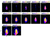 |
Fig. E.2 All detected H2 transitions are presented, except H2 1-1 S(9), which is contaminated by CO ro-vibrational forest. |
 |
Fig. E.3 Spectra extracted form 170 diameter at positions shown on Fig. 1 (top right) and listed in E.2. H2 and HD lines are indicated in blue markers, [Fe II] lines in black markers, and remaining lines are indicated with grey markers and labeled. Spectra between channels were stitched with an additive factor, and the baseline was removed with a manual spline fit. Brightest lines are truncated. |
Measured emission line properties.
All Tables
All Figures
|
Fig. 1 Top left : large-scale view of the BHR71 globule in the Ks (red) and H (green) bands from the Persson Auxiliary Nasmyth Infrared Camera (PANIC; Martini et al. 2004) taken on 2009 January 17 and 18 and in the J (blue) band from the Infrared Side-Port Imager (ISPI; van der Bliek et al. 2004) taken on 2009 June 11 (see also Tobin et al. (2010, 2019)). The stars mark the positions of the protostars from ALMA high-resolution images (Ohashi et al. 2023). The colored rectangles highlight the field of view of the MIRI-MRS mosaics for channels 1 (white), 2 (pink), 3 (yellow), and 4 (red). Top right : MIRI-MRS integrated Gaussian intensity map of H2 S(4) (8.03 μm; color scale) and [Fe II] a6 D9/2-a4F9/2 (5.34 μm; black contours). The circles show and label the regions we selected for spectral analysis. The coordinates are relative to the position of the IR protostar source, 12h01m36.454, −65°08′49″.267 (J2000), which is indicated with the white star. Bottom : integrated Gaussian intensity maps of (from left to right:) [Fe II] a6D9/2-a4F9/2 (5.34 μm; channel 1), H2 S(4) (8.03 μm; channel 2), and [Ne II] 2P3/2-2P1/2 (12.81 μm; channel 3). The final panel on the right shows the thermal dust continuum emission from 19.3 to 19.9 μm (channel 4). The rectangles indicate the field of view of the MIRI-MRS mosaic, and the colors correspond to those in the top left plot. In the bottom right corners, the MIRI-MRS empirical FWHM of the PSF (Law et al. 2023) is indicated as a white circle. |
| In the text | |
|
Fig. 2 MIRI-MRS integrated Gaussian intensity maps of selected atomic and ionic emission lines. The coordinates are relative to the source position of the IR protostar, indicated with the white star. The line quantum identifiers are listed in Table E.3. In the top left corner, regions identified as jet bullets are indicated. In the bottom right corners, the MIRI-MRS empirical FWHM of the PSF (Law et al. 2023) is shown as a white circle. |
| In the text | |
|
Fig. 3 MIRI-MRS integrated Gaussian intensity maps of the representative H2 emission lines of the BHR71-IRS1 outflow. From left to right, we show lines of increasing Eup: H2 v = 1-1 S(5), 10 340 K; H2 v = 0-0 S(7), 7197 K; H2 v = 0-0 S(3), 2503 K; and H2 v = 0-0 S(1), 1015 K. In the bottom right corners, the MIRI-MRS empirical FWHM of the PSF (Law et al. 2023) is shown as a white circle. In the rightmost image, ALMA CO (2-1) integrated emission over the entire blueshifted range (-85; 0 km s−1) with respect to vLSR is shown in color scale. The data presented in Gavino et al. (2024) were taken in May 2021. |
| In the text | |
|
Fig. 4 MIRI-MRS integrated Gaussian intensity maps of molecular lines. For molecules with multiple detected lines, the lines are stacked. Left : rovibrational CO (v = 1-0) map integrated from all unblended lines from channel 1 in 4.9 to the 5.1 μm range. In total, 14 lines are stacked, with Eup = 4725-7338 K. Left middle : CO2, only the Q branch at 14.98 μm (Eup = 964 K) is imaged. Right middle : OH rotational lines integrated over the 15.93-17.80 μm range. A total of 11 lines are stacked with Eup = 7097-14 506 K. Right : OH prompt emission lines from 9.13-9.92 μm. A total of en lines are stacked with Eup = 29 624-48 052 K. |
| In the text | |
|
Fig. 5 MIRI-MRS images of continuum emission from cubes centered on 6.3, 13.8, 19.6, 22.4, and 26.4 μm, from left to right. The images were generated by integrating cubes over 0.6 μm around the central wavelength. The cubes were PSF-subtracted before the imaging. The white star marks the position of the protostar in the mid-IR. |
| In the text | |
|
Fig. 6 Line ratios of selected species at positions B1-B4 plotted as a function of the deprojected distance from the source. Left : ratios of the same species sensitive to the gas temperature: [Co II] 14.5 μm to [Co II] 10.5μm (orange), [Fe II] 17.9 μm to [Fe II] 25.9 μm (blue), and [Ni II] 10.6 μm to [Ni II] 6.6 μm (green). Right : ratios sensitive to the ionization fraction: [Fe II] 25.9μm to [Fe I] 24.0 μm (gray), [Ne II 12.8 μm to [Ar II] μm 6.9 μm (brown), [Cl II] 11.3 μm to [Cl I] 14.4 μm. (pink), and [Ne III] 15.55 μm to [Ne II] 12.8 μm (purple). |
| In the text | |
|
Fig. 7 MIRI-MRS centroid velocity with respect to the vLSR of the protostar and corrected for source inclination for selected emission lines. |
| In the text | |
|
Fig. 8 MIRI-MRS centroid velocity of H2 rotational transitions with respect to the vLSR of the protostar and corrected for the source inclination as a function of Eup. The color shows different positions along the jet (see Fig. 1, top right) |
| In the text | |
|
Fig. 9 Fits to the SED at position B1. The extracted SED was smoothed with a Gaussian kernel. The dashed lines indicate the scattered, warm, and cold dust components, shown in blue, orange, and green, respectively. The solid red line shows the sum of the three blackbodies. The dashed purple line shows the sum of the blackbody temperatures extincted with the KP5 extinction curve. |
| In the text | |
|
Fig. 10 Top : fitted dust temperatures to warm and cold blackbody components for the SEDs in Figs. 9 and B.1. Middle : IR fluxes at 13 and 22 μm as a function of distance from the protostar. The modeled envelope density as a function of radius is shown as the dashed red line (Kristensen et al. 2012). Bottom : surface density of the extincting dust as a function of distance from the protostar. The dashed red line same as in the middle panel. |
| In the text | |
|
Fig. 11 Top : properties of the shock along the jet. Positions B1-B4 are indicated in Fig. 1, and the shock modeling results are summarized in Table D.1. The range of values stems from the density estimate based on S and Cl. Bottom : Fe and Ni abundance at the B1-B4 shock positions based on the shock model as measured in Appendix D. |
| In the text | |
|
Fig. 12 Left : Fe to S elemental ratio compared with the solar abundance (dashed gray line) and non-carbonaceous (NC) and carbonaceous (CC) iron meteorites (green and purple shaded areas, respectively; Grewal et al. 2024). Middle : Ni to S elemental ratio. Right : Ni to Fe elemental ratio. |
| In the text | |
|
Fig. A.1 Images showing an example of the PSF-subtraction. All images are integrated on the 19.3-19.9 μm range, and the color map is scaled to the same min and max values. Left: Original science cube created with ifualign step in the pipeline. Middle: PSF-model centered on the same position as the source centroid, resampled on the same pixel scale, normalized, and multiplied by the maximum value on the science cube per channel. Right: Data with PSF model subtracted. |
| In the text | |
|
Fig. A.2 Spectra extracted from the science data (red), from the PSF-subtracted data (black), and their difference, which is equivalent to the PSF-model spectrum (blue). In the bottom row, the ratio of flux between the PSF model and the science data. The sharp lines in the ratio plot are due to emission lines, which are prominent off-source, but usually fainter at the point source position. |
| In the text | |
|
Fig. A.3 Deprojected positions of the jet measured as a Gaussian centroid fitted to the spatial slice perpendicular to the jet for [Fe II] at 5.34 μm and [Ne II] 12.81 μm. The red curve shows the best fit to Eq. (B.1). Grey dots show the masked region where the expanding internal shock is likely affecting the centroid measurement. |
| In the text | |
|
Fig. B.1 Fits to spectral energy distributions at the positions from PSF-subtracted images. Absorption-subtracted spectra and a best-fit three-component blackbody (red) with components also indicated separately. |
| In the text | |
|
Fig. C.1 Rotational diagrams with extinction correction. Red dots show observed data, blue dots show column densities corrected for extinction following KP5 Pontoppidan et al. (2024) curve. Dashed and dotted lines show fits to warm and hot components, respectively. The solid line shows the sum of the two components. Line intensities of H2 are reported in Table E.3. |
| In the text | |
|
Fig. D.1 Extinction-corrected intensities of [Ne II] (top), [S I] (middle), and [Cl I] (bottom) compared to the shock velocities (x-axis) and densities (black lines) of HM89. Intensities measured at each bullet are marked with the horizontal line. |
| In the text | |
|
Fig. D.2 Extinction-corrected line-intensity ratios shown as point for each region B1-B4 separately. Solid lines refer to the predictions by HM89, which assumed depleted values of the refractory species. Dashed lines show the model predictions rescaled to the Solar values. This is used to estimate the abundances in the BHR71-IRS1 jet. |
| In the text | |
|
Fig. D.3 Extinction-corrected intensity ratios of [Fe II] lines for the B1-B4 bullets. The ratios are plot on a grid of electron temperature (Te), and density (ne) based on NLTE excitation model (Giannini et al. 2013). |
| In the text | |
|
Fig. E.1 Peak brightness of emission line as a function of distance from the protostar, normalized to the maximum value for each line. |
| In the text | |
|
Fig. E.2 All detected H2 transitions are presented, except H2 1-1 S(9), which is contaminated by CO ro-vibrational forest. |
| In the text | |
|
Fig. E.3 Spectra extracted form 170 diameter at positions shown on Fig. 1 (top right) and listed in E.2. H2 and HD lines are indicated in blue markers, [Fe II] lines in black markers, and remaining lines are indicated with grey markers and labeled. Spectra between channels were stitched with an additive factor, and the baseline was removed with a manual spline fit. Brightest lines are truncated. |
| In the text | |
Current usage metrics show cumulative count of Article Views (full-text article views including HTML views, PDF and ePub downloads, according to the available data) and Abstracts Views on Vision4Press platform.
Data correspond to usage on the plateform after 2015. The current usage metrics is available 48-96 hours after online publication and is updated daily on week days.
Initial download of the metrics may take a while.