| Issue |
A&A
Volume 709, May 2026
|
|
|---|---|---|
| Article Number | A120 | |
| Number of page(s) | 20 | |
| Section | Extragalactic astronomy | |
| DOI | https://doi.org/10.1051/0004-6361/202659953 | |
| Published online | 12 May 2026 | |
MUSE-DARK
II. 3D morpho-kinematic modelling of lensed galaxies: Tully-Fisher relation of z ∼ 1 star-forming galaxies
1
Universite Claude Bernard Lyon 1, CRAL UMR5574, ENS de Lyon, CNRS, Villeurbanne F-69622, France
2
Leibniz-Institut für Astrophysik Potsdam (AIP), An der Sternwarte 16, 14482 Potsdam, Germany
3
Observatoire Astronomique de Strasbourg, Université de Strasbourg, CNRS, UMR 7550, 67000 Strasbourg, France
4
French-Chilean Laboratory for Astronomy, IRL 3386, CNRS and Universidad de Concepción, Departamento de Astronomía, Barrio Universitario s/n, Concepción, Chile
5
Aix Marseille Univ, CNRS, CNES, LAM, Marseille, France
6
IRAP, Université de Toulouse, CNRS, CNES, 14 Av. Edouard Belin, 31400 Toulouse, France
★ Corresponding author: This email address is being protected from spambots. You need JavaScript enabled to view it.
Received:
19
March
2026
Accepted:
27
March
2026
Abstract
Extending local kinematic studies to earlier cosmic times is valuable to understand how galaxies evolve in relation to their dark matter haloes. In a series of papers on lensed kinematics, we seek to combine the sensitivity of 3D forward modelling to low signal-to-noise ratio outskirts with the enhanced spatial resolution provided by cluster lensing. In this first paper, we (i) present and validate our methodology, which directly constrains the source parameters by incorporating lensing deflections into the GalPaK3D forward-modelling algorithm, and (ii) investigate the evolution of the stellar-mass and baryonic-mass Tully–Fisher relations (sTFR and bTFR) since z ∼ 1 as a demonstration. We define a robust sample of strongly lensed star-forming galaxies (SFGs) from the MUSE Lensing Cluster survey, spanning magnifications μ = 1.4 − 12.4 and stellar masses M★ = 108.1 − 1010.3 M⊙. Using a series of mock galaxies representative of our sample, we find that our method is significantly more reliable at recovering morpho-kinematic properties than approaches that ignore differential magnification, even for relatively modest magnifications (μ < 6). Restricting the analysis to 95 rotationally supported SFGs with well-constrained velocities, we find a significant evolution of the sTFR zero point (Δ bsTFR = −0.42+0.05−0.05 dex in stellar mass) but no detectable evolution of the bTFR zero point (Δ bbTFR = 0.00+0.06−0.06 dex in baryonic mass) relative to z ≈ 0. Our results are consistent with a mild evolution of the stellar-to-halo mass ratio and support the view that the sTFR has evolved only weakly over the past ∼8 Gyr, aside from shifts driven by the redshift dependence of halo-defining quantities such as the critical density and overdensity. The absence of detectable evolution in the bTFR zero point suggests that the increasing contribution of cold gas mass at higher redshift fully compensates for the evolution observed in the stellar component alone.
Key words: gravitational lensing: strong / methods: data analysis / galaxies: evolution / galaxies: formation / galaxies: high-redshift / galaxies: kinematics and dynamics
© The Authors 2026
 Open Access article, published by EDP Sciences, under the terms of the Creative Commons Attribution License (https://creativecommons.org/licenses/by/4.0), which permits unrestricted use, distribution, and reproduction in any medium, provided the original work is properly cited.
This article is published in open access under the Subscribe to Open model. This email address is being protected from spambots. You need JavaScript enabled to view it. to support open access publication.
1. Introduction
Rotation curves (RCs) provide one of the most direct probes of the total mass profile of a galaxy, which can be contrasted with the visible distribution of its stars and gas. Decades of kinematic studies of nearby disc galaxies, enabled by high-quality RCs, have established a set of empirical results that remain central to current discussions on the physics underlying galaxy evolution. The discovery that the RCs of nearby disc galaxies remain nearly flat out to tens of kiloparsecs (Bosma 1978; Rubin et al. 1978), which is far beyond the radius where a Keplerian decline is expected from visible matter alone, has been key in advancing the standard Λ cold dark matter cosmology (e.g. Mo et al. 1998) as well as alternative gravity theories deviating from Newtonian dynamics at low accelerations (e.g. Sanders & McGaugh 2002; Famaey & McGaugh 2012). Another remarkable finding is their apparent regularity, which manifests in the capacity to generally represent RCs using a universal function of the luminosity and optical scale length (e.g. Persic et al. 1996) as well as in their adherence to tight scaling relations. These include global relations such as the Tully-Fisher relation (TFR; e.g. Tully & Fisher 1977; Bell & de Jong 2001; McGaugh et al. 2000) and Fall relation (Fall & Efstathiou 1980) which extend over several orders of magnitude in stellar mass, as well as local relations such as the radial acceleration relation (e.g. McGaugh et al. 2016). On small scales, the slowly rising RCs of low-mass, dark matter (DM) dominated galaxies imply shallow central DM densities and slopes, challenging the expectations from DM-only halo profiles (Bullock & Boylan-Kolchin 2017, for a review).
Extending local kinematic studies to earlier cosmic times is valuable to understand how galaxies evolve in relation to their DM haloes. Over the past two decades, this effort has been facilitated by sensitive 3D spectrographs across the optical (e.g. VLT/MUSE and Keck/KCWI), near-infrared (e.g. VLT/SINFONI, VLT/KMOS, Keck/OSIRIS, and JWST/NIRSpec), and millimetre (e.g. ALMA and NOEMA) domains. Observations now reveal that disc galaxies at intermediate redshifts (0.5 < z < 3) are reasonably regular albeit dynamically hotter (e.g. Förster Schreiber et al. 2006) and thicker, with scaling relations such as the TFR (Turner et al. 2017; Sharma et al. 2024, and references therein) or Fall relation (e.g. Burkert et al. 2016; Harrison et al. 2017; Swinbank et al. 2017; Bouché et al. 2021) already established (Förster Schreiber & Wuyts 2020, for a review). However, there is no consensus yet as to the outer shape of intermediate-redshift RCs, which is key to constrain DM halo masses: some studies report flat or rising profiles (e.g. Sharma et al. 2021; Puglisi et al. 2023), while others also find declining profiles at large radii (e.g. Lang et al. 2017; Genzel et al. 2017, 2020; Nestor Shachar et al. 2023). The evolution of the stellar-mass TFR is similarly unsettled. In line with earlier results from Sharma et al. (2024), Mancera Piña et al. (2026) reported moderate evidence for a shallower slope at z ∼ 1 compared to the z ≈ 0 relation of Marasco et al. (2025), in tension with expectations if the two galaxy populations share a simple progenitor–descendant relation. A major limitation is that most existing samples span a relatively narrow stellar-mass range (M★ ≳ 109.5 − 10 M⊙; for extensions to lower masses see Contini et al. 2016; Abril-Melgarejo et al. 2021; Mercier et al. 2022), limiting constraints on possible slope evolution. Even when the slope is fixed to local values, conclusions on the evolution of the zero point range from mild evolution if any (e.g. Pelliccia et al. 2017; Tiley et al. 2019), to moderate evolution (e.g. Übler et al. 2017). However, Turner et al. (2017) pointed out that many of these studies can be reconciled with a moderate evolution of the TFR (corresponding to ≃ − 0.4 dex in stellar mass at z ∼ 1, relative to z ≈ 0), once the contribution of pressure support to the dynamics of distant star-forming galaxies (SFGs) is properly included. Finally, constraints on DM density profiles at these epochs remain scarce. Resolving the inner RC calls for high spatial resolution, while constraining the outer RC requires deep observations, making such measurements observationally demanding. With the exception of Bouché et al. (2022), Ciocan et al. (2026), and Danhaive et al. (2026, which relies on slitless spectroscopy), most existing studies focus on relatively massive SFGs with M★ ≳ 1010 M⊙ (e.g. Genzel et al. 2020; Nestor Shachar et al. 2023).
Disentangling physical evolution from observational biases remains challenging. Kinematic measurements primarily rely on molecular or warm ionised gas, sometimes supplemented by stellar kinematics (Guérou et al. 2017; Straatman et al. 2022; Übler et al. 2024; Muñoz López et al. 2024). Unlike HI, those tracers generally do not reach far beyond the optical disc, but studies of individual galaxies in HI are not yet feasible because of the intrinsic faintness of the 21 cm line. In addition, distant SFGs are apparently and intrinsically fainter, smaller (e.g. van der Wel et al. 2014; Nedkova et al. 2021), and more turbulent (e.g. Wisnioski et al. 2025). Marginal spatial resolution leads to beam smearing, which smooths out velocity gradients and inflates the observed velocity dispersion (Epinat et al. 2008, for an extensive analysis), while cosmological dimming limits the signal-to-noise ratio (S/N) achievable in typical exposure times. Forward-modelling tools that include observational effects, such as GalPaK3D (Bouché et al. 2015a,b), DysmalPy (Price et al. 2021; Lee et al. 2025, and references therein), 3DBarolo (Di Teodoro & Fraternali 2015), or qubefit (Neeleman et al. 2020, 2021), help mitigate those limitations by leveraging the full 3D information in the data (see Lee et al. 2025; Yttergren et al. 2025, for comparisons). Nonetheless, limited spatial resolution can still wash out kinematic features (see the validation tests in Bouché et al. 2015b; Di Teodoro & Fraternali 2015) and sometimes result in misclassifications (Leethochawalit et al. 2016; Simons et al. 2019). Combined with typically small sample sizes, this complicates comparisons with both local and other high-redshift datasets.
Attempts to overcome these limitations have used either adaptive optics (e.g. Förster Schreiber et al. 2018) or gravitational lensing (e.g. Girard et al. 2020) to achieve ≃1 − 4 kpc resolution at high redshift. Near-diffraction-limited adaptive optics observations remain restricted to small samples and/or relatively massive SFGs, since deep integrations are performed on a target-by-target basis. Cluster-lensed observations do not face this constraint, but they require additional modelling to recover intrinsic source properties. Previous kinematic studies of lensed SFGs have mostly analysed source-plane reconstructions of the datacubes (e.g. Jones et al. 2010, 2013; Swinbank et al. 2011; Livermore et al. 2015), or fitted kinematic parameters directly in the image plane (e.g. Di Teodoro et al. 2018; Girard et al. 2018, 2020), and in some cases included a global correction to account for the lensed axis ratio (e.g. Mason et al. 2017). A handful of studies have incorporated lensing deflections directly in their kinematic modelling. Patrício et al. (2018) proposed a forward-modelling approach accounting for the point-spread function (PSF) and lensing deflections on resolved velocity and metallicity maps. Rizzo et al. (2018) developed an algorithm that jointly infers the lens mass model and the source kinematics from the same datacube, although this was applied to galaxy or group-scale lenses with comparatively simple lens mass distributions. Another tool that includes the modelling of galaxy-scale lenses as well as source kinematics is described in Chirivì et al. (2020). Finally, we highlight Liu et al. (2023) who developed a lensing transformation module to complement the DysmalPy 3D algorithm.
In this series of papers on lensed kinematics, we combine the capacity of 3D algorithms to collectively exploit peripheral (hence, low S/N) spaxels with the enhanced spatial resolution enabled by cluster gravitational lensing to study the kinematics of intermediate-redshift galaxies. We extend GalPaK3D to include lensing deflections directly in the forward model, enabling direct comparison between the model and the observed data, rather than intermediate products (reconstructed datacubes or moment maps) whose correlated pixels are known to introduce systematics1. We model the kinematics of a sample of 116 [O II] emitters drawn from the MUSE Atlas of Lensing Clusters (Richard et al. 2021, hereafter R21), spanning the redshift range 0.5 < z < 1.5. This first paper focuses on the methodology and sample definition, and investigates the evolution of the stellar-mass and baryonic-mass Tully–Fisher relations (sTFR and bTFR) since z ∼ 1 as a demonstration.
This paper is organised as follows. We begin with a brief overview of the MUSE Lensing Cluster Survey and the Frontier Fields ancillary data (Sect. 2). We then describe the implementation of our strong-lensing kinematic modelling with GalPaK3D (Sect. 3) and assess its recovery performance using mock datacubes (Sect. 4). Next, we define and characterise our kinematic sample (Sect. 5) and use it to investigate the sTFR and bTFR at intermediate redshift (Sect. 6). The results are discussed in Sect. 7, and our conclusions are summarised in Sect. 8.
Throughout this analysis, we assume a standard Λ cold dark matter cosmology with Ωm = 0.3, ΩΛ = 0.7, and H0 = 70 km s−1 Mpc−1. Unless specified otherwise, we adopt a Bayesian approach and report best-fit parameters as the median of their posterior distribution. Stellar masses and star formation rates (SFRs) are derived assuming a Chabrier (2003) initial mass function (IMF), or converted to this IMF where necessary.
2. Data and cluster mass models
The sample of [O II] emitters used in this analysis is a subsample of the MUSE Atlas of Lensing Clusters2 R21, a legacy programme targeting the central region of 19 massive galaxy clusters with the MUSE instrument (Bacon et al. 2010). In this study, we focus on four clusters that are part of the Frontier Fields, which benefit from extensive ancillary data: Abell 2744, Abell 370, Abell S1063, and MACS0416. We summarise the key features of the MUSE observations and ancillary datasets below and in Table A.1.
2.1. The MUSE parent sample of lensing clusters
The MUSE Atlas of Lensing Clusters combines data acquired with integral-field spectroscopy (IFS) spanning the 475 − 930 nm range with a spatial sampling of 0.2″ × 0.2″, a spectral sampling of 1.25 Å, and a spectral resolution from ℛ = 1800 to ℛ = 3600. The final datacubes combine exposures taken in both standard and ground-layer adaptive optics (Ströbele et al. 2012) modes, yielding effective integration times of 2 − 15 h per pointing. For the four Frontier Fields clusters, the resulting PSF has a median full width at half maximum (FWHM) of 0.65″ at 7000 Å, corresponding to an intrinsic spatial resolution of  and a sampling of
  at z ∼ 1, where μ is the lensing magnification factor. The multiple-image regions were covered with four adjacent pointings for Abell 370 and Abell 2744, and two pointings for Abell S1063 and MACS0416. Data reduction largely followed the standard procedure of Weilbacher et al. (2020), with some adaptations to cope with the high density of extended bright sources in lensing cluster fields. The observing and data reduction strategies are detailed in R21 for the first twelve clusters, including Abell 2744, Abell 370, and MACS0416, and in Claeyssens et al. (2022) for five additional clusters, including Abell S1063.
2.2. Ancillary data
In addition to the MUSE data products, this study relies on the wealth of observations targetting the Frontier Fields. The HFF-DeepSpace project (Shipley et al. 2018) combined Hubble Space Telescope (HST) ACS and WFC3 imaging with Ks-band observations from the KIFF survey (Brammer et al. 2016), obtained using VLT/HAWK-I and Keck/MOSFIRE. Together, those datasets provide uniform multi-wavelength coverage in up to 17 filters, spanning the UV to the NIR, and are supplemented by post-cryogenic Spitzer/IRAC imaging at 3.6 μm and 4.5 μm (and archival 5.8 μm and 8.0 μm data where available). The catalogues also include images where the light of bright cluster galaxies (BCGs) has been modelled and subtracted, enabling the detection and analysis of faint background sources. For the purposes of this work, we make use of the HFF-DeepSpace photometric catalogues along with BCG-subtracted images sampled at 0.06″ per pixel and their corresponding empirical PSFs obtained by stacking isolated and unsaturated stars.
2.3. Cluster mass models
To study the intrinsic properties of the lensed galaxies, we used the parametric cluster mass models from Mahler et al. (2018), Lagattuta et al. (2019), R21 and Beauchesne et al. (2024) (see Table A.1), constructed with the public Lenstool software (Kneib et al. 1996; Jullo et al. 2007). These models were constrained by numerous multiple-image systems identified in the MUSE and HST catalogues, including both spectroscopically confirmed sources and continuum sources in unambiguous lensing configurations.
Each cluster mass model was built iteratively using pseudo-isothermal elliptical potentials, starting from a few cluster-scale potentials optimised to reproduce the most secure multiple-image systems, and progressing to galaxy-scale potentials whose shapes were scaled according to the light distribution of cluster members (assuming a constant mass-to-light ratio). For the four Frontier Fields clusters, the models were constrained with 29 − 71 secure multiple-image systems, achieving a typical error of 0.6 − 0.8″ rms in reproducing the observed images. Statistical uncertainties on the model parameters were estimated via Markov chain Monte Carlo (MCMC) sampling of the posterior distribution. From these models, we derived two key products for our analysis: lensing magnification maps and deflection maps, which provide the angular displacement between image plane and source plane positions at a given source redshift, allowing us to correct both flux magnification and shape distortions in the lensed galaxies.
3. GalPaK3D Strong Lensing Extension
For this study, we extracted the intrinsic morphology and kinematics of distant SFGs using an extension of the 3D forward-modelling tool GalPaK3D, which simulates lensed emission-line datacubes from a parametric rotating disc model. Building on the standard GalPaK3D algorithm, we adapted the forward-modelling coordinate transformations to include lensing deflections. The extension proceeds as follows (Fig. 1).
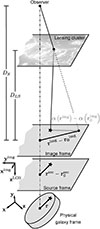 |
Fig. 1. Schematic view of the lensing configuration and coordinate frames. The observed image-frame coordinates rimg − r0img are mapped to source-frame coordinates rsrc − r0src via the lens equation |
3.1. Image-frame coordinate cube construction
First, a 3D coordinate cube is generated in the image frame Rimg = (rimg, zLOS), where rimg = (ximg, yimg) are the sky coordinates, defined on an oversampling of the observed IFS datacube grid, and zLOS is the spatial coordinate along the line of sight (LOS). The model grid is typically oversampled by a factor of two to mitigate discretisation errors. We emphasise that subsequent transformations act on the spatial coordinates stored in the cube, while the grid itself remains aligned and regularly sampled along the IFS spatial axes and the LOS.
3.2. Image-plane centring
Coordinates are then expressed relative to the galaxy centre, R0img = (r0img, z0LOS). Here, r0img = (x0img, y0img) corresponds to the sky coordinates of the apparent galaxy centre fitted by GalPaK3D, and z0LOS is set such that the galaxy centre lies in the middle of the model cube along the LOS. For multiply imaged systems, fitting the apparent centre of one counter-image is sufficient to reproduce the full system within the accuracy of the lens model.
3.3. Source-plane mapping
Using the lens equation, the coordinates stored in Rimg − R0img are mapped to the source plane and expressed relative to the galaxy centre as Rsrc − R0src = (rsrc − r0src, zLOS − z0LOS),
![Mathematical equation: $$ \begin{aligned} \mathbf r ^\mathrm{src} - \mathbf r _0^\mathrm{src} = \left[ \mathbf r ^\mathrm{img} - \mathbf r_0 ^\mathrm{img} \right] - \left[\boldsymbol{\alpha } \left( \mathbf r ^\mathrm{img} \right) - \boldsymbol{\alpha } \left( \mathbf r _0^\mathrm{img} \right) \right] , \end{aligned} $$](/articles/aa/full_html/2026/05/aa59953-26/aa59953-26-eq6.gif) (1)
(1)
where α is the user-provided deflection angle resulting from the cluster lens model. Lens models commonly include reduced deflection maps  , defined such that
  , where DLS and DS are the angular-diameter distances from the lens to the source and from the observer to the source, respectively. A bilinear interpolation is used to derive
  from the pixelated deflection maps. The result is a cube storing source-frame coordinates, regularly sampled in the image frame.
3.4. Rotation into the physical galaxy frame.
The source-frame coordinates are then rotated into the physical galaxy frame, R = (r,z), where r = (x,y) lies in the galaxy midplane and z is the coordinate along the direction perpendicular to it. This transformation is performed by applying two successive 3D rotations to the source-frame coordinates: a rotation ℛz(PA) about the z-axis to account for the position angle (PA), followed by a rotation ℛx(i) about the x-axis to account for the inclination i,
 (2)
(2)
The resulting coordinates are expressed in the physical galaxy frame. The following steps then proceed as in the standard GalPaK3D algorithm, except that an oversampled model cube is continued to be used to minimise discretisation errors. We summarise them for self-consistency.
3.5. Flux and kinematic profile assignment
Parametric flux and velocity profiles are applied to the galaxy-frame coordinates cube, that is, each pixel of the cube is allocated a flux or a rotational velocity vector corresponding to its coordinates in the galaxy frame. A flux cube is created from a radial profile I(r) and a vertical profile I(z) relying on a half width at half maximum hz. The rotational velocity field V⊥(R) = (vx, vy, 0) is generated from a rotation velocity profile v⊥(r,z) and assumes circular orbits. The RC can be modelled using a simple parametrisation, such as the arctan model (Courteau 1997) adopted in this paper, or a more detailed disc-halo decomposition (Bouché et al. 2022; Ciocan et al. 2026).
3.6. Derivation of moment maps
The flux cube and velocity field are used to generate flux, LOS velocity and LOS velocity dispersion moment maps.
-
The flux map is obtained directly by collapsing the flux cube along the LOS.
-
The LOS velocity map is derived from a LOS velocity cube. At each position, the LOS component of the velocity field is computed as
 (3)
(3)following the coordinate transformations of the previous steps. z0λ is the systemic spectral position (fitted by GalPaK3D), and Δv is the velocity increment per spectral pixel. The LOS velocity map is then obtained as the flux-weighted mean of this vLOS cube along the LOS.
-
The LOS velocity dispersion map combines three contributions in quadrature: from the disc self-gravity σd(r) (with σd(r)/hz = V⊥(r)/r for thick discs); a projection term due to the blending of different velocities along the LOS, computed from the flux-weighted variance of the vLOS cube along the LOS; and a constant and isotropic floor σ0 fitted by GalPaK3D.
3.7. Model cube construction
A model cube in observational coordinates  is built by assigning, at each spaxel, a Gaussian line (or doublet) profile with the flux, velocity, and velocity dispersion defined by the corresponding moment maps. This model cube is free from instrumental resolution.
3.8. Convolution with the instrumental response and comparison to data
Finally, the model cube is convolved with the instrumental response: a 3D kernel combining the PSF and the line spread function (LSF). The oversampled cube is re-binned before being compared with the data  .
.
With this end-to-end modelling approach, the morphological and kinematic parameters inferred by GalPaK3D are implicitly corrected for lensing distortions and observational effects such as beam smearing.
Among the algorithms implemented in GalPaK3D, we adopted the MultiNest (Feroz et al. 2009; Buchner 2016) Bayesian inference tool to sample the posterior distribution of the parameters θ given the data 𝒟. This sampler provides an efficient and robust sampling strategy for high-dimensional parameter spaces. Throughout this study, the runs were performed with 200 live points, a sampling efficiency of 0.8, and an evidence tolerance of 0.5. We defined a likelihood function as  , with
![Mathematical equation: $$ \begin{aligned} \chi _{\rm 3D}^2 = \sum _\mathbf{r ^\mathrm{img}, z^\lambda } \frac{\left[ I_{\rm obs} \left(\mathbf r ^\mathrm{img}, z^\lambda \right) - I_{\rm mod} \left(\mathbf r ^\mathrm{img}, z^\lambda \right) \right]^2}{\mathrm{Var}\left[ I_{\rm obs} \right]\left(\mathbf r ^\mathrm{img}, z^\lambda \right)}. \end{aligned} $$](/articles/aa/full_html/2026/05/aa59953-26/aa59953-26-eq15.gif) (4)
(4)
The posterior distribution is then given by the Bayes theorem  , where
  is the overall prior corresponding to the product of the individual priors.
4. Recovery performance using mock datacubes
In this section, we examine:
-
(i)
The robustness of our method when applied to datacubes with limited S/N, spatial and spectral resolution;
-
(ii)
How our results compare with those obtained using a kinematic model that does not account for differential magnification, in other words, when parameters are inferred in the image frame and, where relevant, simply rescaled by the magnification factor (e.g. Di Teodoro et al. 2018; Girard et al. 2018, 2020).
To this end, we evaluated the performance of the GalPaK3D Strong Lensing Extension on a series of mock datacubes representative of our sample (Sect. 5), generated with its forward-modelling capability.
4.1. Datacube generation
Synthetic galaxies were assigned a redshift drawn from a uniform distribution and stellar masses sampled from the star-forming stellar mass function at z ∼ 1 (Weaver et al. 2023). Other physical properties (e.g. effective radius, SFR, velocity, velocity dispersion) were set by scaling relations and their scatter, following a procedure comparable with Lee et al. (2025).
The [O II] emission, used as the kinematic tracer, was assumed to follow the stellar disc. We adopted an exponential surface brightness profile (Sérsic index n = 1) with an effective radius Re from the stellar mass–size relation of Nedkova et al. (2021), corrected to rest-frame I band (van der Wel et al. 2014), and a Gaussian vertical profile with scale height  (Lian & Luo 2024; Tsukui et al. 2025).
The RC was described by an arctan function (Courteau 1997),
 (5)
(5)
where vmax is the asymptotic velocity and rt the turnover radius. Velocities were defined at 1.8Re (the radius enclosing 80% of the total light for an exponential disc). In practice, we drew v1.8 = vc(1.8Re) from the local TFR reported by Turner et al. (2017) and based on the reference sample of Reyes et al. (2011), and used it to derive vmax. The turnover radius was set to rt = Rd/1.8, with Rd = Re/1.68 the disc scale length, as derived by Bouché et al. (2015b) from the observed scaling between galaxy size and inner velocity gradient (Amorisco & Bertin 2010).
The typical velocity dispersions of z ∼ 1 galaxies (10 − 60 km/s, Wisnioski et al. 2025) indicate that turbulent motions provide significant pressure support to the ionised gas, counteracting gravity. As a result, the observed rotation velocity traced by [O II] is lower than the circular velocity, that is, the velocity a test particle would have if it were purely supported by gravity. We therefore included a pressure-support correction to the circular velocity profile, following the prescription of Dalcanton & Stilp (2010) for an exponential radial gas distribution,
 (6)
(6)
where σr2(r)≈[hzvc(r)/r]2 + σ02. The value of σr(1.8Re), from which σ0 is derived, was assigned following the redshift evolution measured by Übler et al. (2019).
For each realisation, we drew a random position and sky orientation within 1′ of the brightest cluster galaxy in Abell 370, and constructed a  (20 × 32 × 32 px) synthetic MUSE datacube assuming the lensing model of Lagattuta et al. (2019). The mock galaxy was centred in the cube and assigned a random inclination drawn from a uniform distribution in cos(i), restricted to i > 30°, and oriented at a near-diagonal angle relative to the cube axes. Its SFR was drawn from the star-forming main sequence of Boogaard et al. (2018) and converted to a total [O II] luminosity using the calibration of Gilbank et al. (2010),
![Mathematical equation: $$ \begin{aligned} \begin{aligned} L_{\rm [OII]} = \mathrm{SFR} &\times \left( a \times \tanh \left[(x-b)/c \right] + d \right) \\&\times 1.06 \times 2.53\,\times \,10^{40}\,\mathrm{erg\,s}^{-1}, \end{aligned} \end{aligned} $$](/articles/aa/full_html/2026/05/aa59953-26/aa59953-26-eq22.gif) (7)
(7)
where L[OII] is the luminosity of the [O II] doublet in erg s−1, x = log(M★/M⊙), (a, b, c, d) = (−1.424, 9.827, 0.572, 1.700), and the factor 1.06 is used to convert the Gilbank et al. (2010) calibration from a Kroupa (2001) IMF to a Chabrier (2003) IMF assumed in Boogaard et al. (2018). The [O II] emission was modelled as a double Gaussian with a fixed flux ratio r[OII] = Fλ3727/Fλ3729 = 0.7.
We generated a datacube free from instrumental resolution with an initial sampling of 0.04″ × 0.04″ (that is, oversampled by a factor of 5), and used it to compute the luminosity-weighted magnification. To reproduce the observed magnification distribution (see Fig. 10 of R21), we accepted or rejected mocks based on a probability density function proportional to μ−2 and imposing 1.5 < μ < 6. The lower limit accounts for the limited spatial coverage of the MUSE data, while the upper limit ensures that mock galaxies remain within a reasonable datacube size.
For each accepted galaxy, the datacube was convolved with the PSF model from R21, the Gaussian LSF model from Bacon et al. (2017), and resampled to the MUSE spatial sampling (0.2″ × 0.2″). Gaussian white noise was then added to each pixel to match the surface-brightness limit corresponding to a 2-hour exposure time in R21. We generated 3000 mock galaxies following this procedure, and measured the maximum S/N (S/Nmax) by fitting the [O II] doublet in the central spaxel. We retained only galaxies with an effective S/N (introduced in Sect. 4.2)  , where RPSF is the PSF half width at half maximum, and satisfying v1.8/σ0 > 1. This selection yielded a final sample of 1923 mock galaxies.
4.2. Recovery performance
We extracted the kinematics of our mock galaxies twice: first using a kinematic model similar to the one employed for its generation, but with an oversampling factor of 2 instead of 5 to reduce computation time; and second, treating the galaxy as if it were not lensed, with the resulting parameters simply rescaled by the magnification factor where relevant. In both cases, we assumed that the true PSF and LSF are known without error3. The adopted priors are summarised in Table 1.
Main parameters of our kinematic model, together with their adopted priors or fixed values.
Fig. 2 shows the relative errors in the recovered parameters, defined as δp/p = (pfit − ptrue)/ptrue. Fig. 3 presents the same quantities but is restricted to mock galaxies with magnifications μ > 3. In both figures, the relative errors are plotted as a function of S/Nmax scaled by a power α of the apparent size-to-PSF ratio  .
.
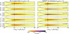 |
Fig. 2. Comparison of the relative errors in the inferred properties, defined as δp/p = (pfit − ptrue)/ptrue, for a kinematic model fitted either directly in the image frame (left column) or in the source frame using the GalPaK3D Strong Lensing Extension (right column). Each row shows the error density distribution for a given property, restricted to the rotation-dominated subsample of mock galaxies (v1.8/σ0 > 1). The effective radius is corrected a posteriori by the magnification when fitted in the image plane. The PA error is relative to PAtrue = 130°, as in Bouché et al. (2015b). Dashed lines show the empirical relation |


In the marginally resolved regime (Re/RPSF ≃ 1), the accuracy of recovered properties is known to depend not only on the S/N but also on the compactness of the source relative to the PSF. For blank-field galaxies, Bouché et al. (2015b) showed that the relative uncertainties in Re, PA, i, and vmax scale inversely with both the central surface brightness (or S/N) and (Re/RPSF)α, with α ≃ 0.8, 1.2, 1.4, and 0.8, respectively. They therefore introduced an effective S/N, S/Neff = S/Nmax × (Re/RPSF), to capture this dependence.
When modelling our mock galaxies with the GalPaK3D Strong Lensing Extension, we recovered similar trends4 with S/Nmax and apparent size-to-PSF ratio (indicated by the dashed lines in the figures). This indicates that, once differential magnification is properly accounted for, the relative errors scale approximately as μ−α/2 within the magnification range explored here. In contrast, this behaviour is much less apparent when fitting directly in the image plane, particularly for the higher-magnification subsample shown in Fig. 3. This suggests that neglecting differential magnification introduces a limiting source of error that cannot be mitigated by increased S/N alone.
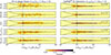 |
Fig. 3. Same as Fig. 2, but additionally restricted to the subsample of mock galaxies satisfying μ > 3. |
For galaxies satisfying  , both approaches yield negligible median deviations (within 5%) for most parameters. The main exception is the effective radius, which is biased by +9% when fitted directly in the image plane. In terms of relative error, ignoring (accounting for) differential magnification results in standard deviations of 31% (8%) for Re, 59° (49°) for the PA, 16% (4%) for the inclination, 18% (14%) for v1.8, and 25% (15%) for σ0.
The benefits of including lensing deflections in the forward modelling become more pronounced at higher magnifications. Restricting the analysis to 3 < μ < 6, we find that direct image-plane fitting leads to significant median deviations even for objects with  , namely +14% for Re, +6% for the inclination, and −7% for v1.8. The corresponding standard deviations in the relative errors increase to 44% for Re, 70° for the PA, 18% for the inclination, 20% for v1.8, and 38% for σ0 when differential magnification is ignored, compared to 10%, 50°, 5%, 14%, and 11%, respectively, when it is accounted for.
Finally, we restricted the sample to mock galaxies with apparently well-constrained velocities for both fitting approaches, defined by  , where Δv1.8 is the posterior standard deviation. Even in this case, fitting directly in the image plane yields a significant median deviation of +10% in Re. The corresponding standard deviations in the relative errors, ignoring (accounting for) differential magnification, are 28% (7%) for Re, 27° (7°) for the PA, 17% (4%) for the inclination, 14% (8%) for v1.8, and 27% (16%) for σ0.
Overall, those validation tests demonstrate that the intrinsic morpho-kinematic properties of strongly lensed SFGs can be reliably recovered for rotation dominated (v1.8/σ0 > 1) galaxies which satisfy  , with α ≃ 1. We note that the recovered parameters exhibit relative uncertainties comparable to those obtained in the unlensed case at similar S/Neff, when differential magnification is accounted for. We find that this approach is significantly more robust, particularly for morphological parameters and velocity dispersion, with improvements of factors ≃2 − 4 in relative errors, than methods that neglect differential magnification, even for moderate magnifications (μ < 6). Circular velocity also benefits from this approach, albeit to a lesser extent, as the improved inclination recovery entails a more accurate deprojection of the observed velocity field.
5. A robust sample of strongly lensed SFGs observed with MUSE
5.1. Sample definition
Our sample selection is guided by data quality and by the ability of our morpho-kinematic modelling approach to robustly recover source properties. As shown in Sect. 4, the relative error of recovered parameters scales approximately with  . In the following paragraphs, we detail how it is measured and present our sample selection, which consists of a series of cuts based on S/Neff and other observational properties. We also present complementary measurements (e.g. single and double-Sérsic modelling) to better characterise the sample and to assess the consistency of our morpho-kinematic results relative to parameters inferred from broadband imaging.
We started by extracting a base sample of [O II]λλ3727, 3729 emitters from the MUSE Lensing Cluster catalogues of Abell 370, Abell 2744, MACS0416 and Abell S1063, retaining only sources with a secure redshift estimate (ZCONF = 3). The spectral coverage of MUSE limits the redshift range, which we further restricted to exclude cluster members (z = 0.3 − 0.5). The resulting sample comprises galaxies with 0.5 < z < 1.5. We then matched this sample with the photometric catalogue of Shipley et al. (2018) and visually inspected the detections to remove duplicates from segmentation errors, galaxies located at the edges of the MUSE mosaic, galaxy–galaxy lensed systems, and perturbed galaxies showing tidal features.
5.1.1. Lensing magnification and morphological properties
For each galaxy, we measured the gravitational lensing magnification and intrinsic structural parameters within a manually defined region chosen to prevent contamination from neighbouring galaxies. Deflection and magnification maps were generated from the cluster mass models referenced in Table A.1, and the galaxy magnification was computed as the harmonic mean within the useful region.
We then forward-modelled the H-band (HST/WFC3 F160W, rest-frame I band) flux distribution using the cleanlens mode of the Lenstool software. The intrinsic surface brightness was modelled as a single Sérsic (1963) profile with seven free parameters: centre position, magnitude, scale radius, Sérsic index n, PA, and ellipticity ϵ. The model flux distribution was lensed with the corresponding lensing mass model, convolved with the empirical F160W PSF from Shipley et al. (2018), and combined with a sky background estimated via 3σ-clipping to produce a model image-frame flux distribution. MCMC sampling was used to compare the modelled and observed distributions, and to obtain the posterior distributions of the model parameters assuming broad uniform priors. From these, we derived the intrinsic effective radius and the source-frame axis ratio qsrc = (1 − ϵ)/(1 + ϵ). We computed the inclination i, assuming cos2(i) = (q2 − q02)/(1 − q02) with an intrinsic stellar disc axis ratio q0 = 0.25 (Lian & Luo 2024; Tsukui et al. 2025). For visualisation, we also performed a direct source reconstruction by mapping image pixels onto a regular source pixel grid.
5.1.2. S/N and kinematics of the [O II] line
To prepare the MUSE data for kinematic analysis, we extracted 100 Å sub-datacubes centred on the [O II] doublet, using the positions and spectroscopic redshifts from R21. We masked the central 25 Å and fitted the continuum in each spaxel as a linear ramp between the mean flux bluewards and redwards of the doublet. After subtracting the continuum, we cropped the sub-datacubes to the central 25 Å.
We then derived kinematic maps to visually inspect the velocity fields. We adaptively binned spaxels to a target S/N of ≃5 using the PowerBin algorithm (Cappellari 2025). To ensure that the binning maximises the S/N in the outer regions, we first retained only spaxels with S/N > 2, where the S/N is estimated from a [O II] pseudo–narrowband image smoothed with a Gaussian kernel (σ = 1 spaxel). In each resulting bin, the [O II] doublet was modelled with two Gaussian components sharing a common velocity and velocity dispersion. The flux, velocity, and velocity dispersion were inferred using Bayesian sampling with the affine-invariant MCMC ensemble sampler emcee (Foreman-Mackey et al. 2013), using 10 walkers run for 10 000 steps, including a burn-in of 2000 steps. For reference, we also fitted the [O II] doublet in the brightest individual spaxel to estimate S/Nmax.
5.1.3. Selection criteria
Our final sample is defined by the following criteria:
-
Secure spectroscopic redshift (ZCONF = 3) with 0.5 < z < 1.5;
-
No evidence of gravitational perturbations (e.g. tidal arms), edge effects, or contamination, based on visual inspection.
For robust kinematic recovery, we additionally required:
-
 ;
; -
 , that is, the stellar disc must span at least one resolution element;
 -
i > 30 deg, excluding face-on galaxies.
Our selection (Fig. 4) comprises 116 galaxies excluding 8 counter-images of galaxies already in the sample. For these cases where two counter-images of the same galaxy pass our selection criteria, we excluded the counter-image with the lower S/Neff from the final sample.
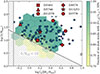 |
Fig. 4. S/N of the brightest [O II] spaxel against the apparent size-to-PSF ratio. The hatched grey region marks the parameter space excluded by our selection. Red symbols mark 6 galaxies chosen to showcase the range of apparent sizes and S/N in Fig. 6. Open symbols mark galaxies that are either dispersion-dominated (v1.8/σ0 ≤ 1) or have poorly constrained velocities (Δv1.8/v1.8 ≥ 30%), where Δv1.8 is the posterior standard deviation. The background hexagonal bins illustrate the fraction of rotation-dominated (v1.8/σ0 > 1) mock galaxies with a robust velocity recovery ( |
5.2. Additional measurements
5.2.1. Bulge-to-total flux ratio
We estimated the bulge-to-total flux ratio (B/Tflux) by re-modelling the H-band flux distribution with a two-component bulge–disc model, following the general steps of Sect. 5.1.1. We adopted an exponential disc (nd = 1) plus a de Vaucouleurs bulge (nb = 4), with shared centre, PA, and ellipticity. Initial guesses and constraints were drawn from the single-Sérsic fit. Notably, the disc (bulge) effective radius was forced to be larger (smaller) than the single-component effective radius. This model has eight free parameters: common centre, PA, and ellipticity, plus distinct magnitudes and scale radii for the bulge and disc. We inferred B/Tflux from the posterior probability distribution samples.
5.2.2. Stellar population properties
Stellar population properties were derived from spectral energy distribution (SED) modelling using the photometry of Shipley et al. (2018). Their catalogues provide fluxes corrected to total fluxes based on the ratio of SExtractor’s AUTO flux to an aperture flux in the F160W filter. To ensure stellar masses and SFHs consistent with our morphology and kinematics measurements, we applied an additional aperture correction: for each band, the Shipley et al. (2018) flux was scaled by the ratio of the total F160W flux derived from the best-fit Lenstool bulge–disc model (Sect. 5.2.1) to the reported F160W flux, both similarly corrected for Galactic extinction. For galaxies segmented across multiple catalogue entries, we combined the corresponding fluxes and uncertainties before applying this correction.
We then removed invalid flux values, corrected the fluxes and uncertainties for lensing magnification, and imposed a minimum relative uncertainty of 5% except for Spitzer/IRAC channels where we imposed 10%. This error floor, following Carnall et al. (2018, 2019), was intended to prevent underestimating uncertainties in the high-S/N regime, where calibration errors dominate the photometric error. We did not include magnification uncertainties at this stage, as doing so would unphysically allow the model spectral slope to vary within the magnification error range.
For each galaxy, we fitted the SED at the spectroscopic redshift estimate of R21, using the Bayesian spectral fitting code BAGPIPES (Carnall et al. 2018). Our model relies on the 2016 version of the Bruzual & Charlot (2003) stellar population synthesis models with a Kroupa (2001) IMF, a free metallicity and the Calzetti et al. (2000) reddening law. Following Leja et al. (2019a,b), we adopted a nonparametric SFH divided into seven bins of lookback time, with the SFR constant within each bin and linked by a continuity prior to disfavour sharp transitions between bins. The bins are defined at 0–30, 30–100, 100–330, 330–1100 Myr, and 0.85tuniv–tuniv, where tuniv is the age of the Universe at the observed redshift. The remaining two bins are equally spaced in logarithmic time between 1100 Myr and 0.85tuniv. The model parameters and their priors are summarised in Table 2.
Parameters of our SED model, together with their adopted priors or fixed values.
We applied corrections of −0.034 dex and −0.027 dex to convert our stellar masses and SFRs, respectively, to a Chabrier (2003) IMF (Madau & Dickinson 2014).
5.3. General sample properties
The general properties of our sample (Fig. 5) are broadly representative of main-sequence SFGs over 0.56 ≤ z ≤ 1.37 and 8.1 ≤ log(M★/M⊙) ≤ 10.3, observed under moderate magnification in the range 1.4 ≤ μ ≤ 12.4 (5th–95th percentiles). The lower tail of the effective radius distribution is under-represented in our selection, leading to an overall +0.08 dex offset relative to the size-mass relation of Nedkova et al. (2021). In terms of structural parameters, we note that the majority of our sample is disc-dominated with 70% of galaxies having B/Tflux < 0.3. This disc-dominated subset has nearly exponential light profiles as observed in the H band (rest-frame I band), with a median Sérsic index of 1.0. We compare the properties of the mock sample and the kinematic sample in Fig. B.1.
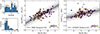 |
Fig. 5. General sample properties. The panels show the distributions of redshift (top left) and magnification (bottom left), together with the locations of the galaxies in the M★–SFR (middle) and M★–Re (right) planes. Effective radii are corrected to rest-frame 5000 Å following Eqs. 1 and 2 of van der Wel et al. (2014), expressed relative to the size–mass relation of Nedkova et al. (2021) (interpolated with redshift), and scaled to z = 1. Similarly, SFRs are expressed relative to the star-forming main sequence of Boogaard et al. (2018), adjusted to the redshift and stellar mass of each galaxy, and normalised to z = 1. The shaded regions indicate the ±1σ (dark grey) and ±2σ (light grey) scatter around the corresponding relations. Open symbols and histogram segments mark galaxies that are either dispersion-dominated (v1.8/σ0 ≤ 1) or have poorly constrained velocities (Δv1.8/v1.8 ≥ 30%), where Δv1.8 is the posterior standard deviation. |
6. Derivation of the TFR at z ∼ 1
6.1. Morphology and kinematics of the sample
We extracted the kinematics of our sample using the model described in Sect. 4 and the main priors listed in Table 1. The model comprises 12 free parameters, ![Mathematical equation: $ \boldsymbol{\theta} = \{\mathbf{r}_0^{\mathrm{img}}, z_0^\lambda, F^{\mathrm{[OII]}}, R_e, n, i, \mathrm{PA}, \sigma_0, r_t, v_{\mathrm{max}}, r^{\mathrm{[OII]}}\} $](/articles/aa/full_html/2026/05/aa59953-26/aa59953-26-eq37.gif) , which jointly describe the apparent position and flux, together with the intrinsic structural properties and kinematics (corrected for pressure support). For the inclination, we adopted a Gaussian prior centred on the single-Sérsic H-band estimate (iF160W, see Sect. 5.1.1), with a scatter of 5 deg and truncated at ±15 deg. We additionally restricted the centre position to ±1 spaxel around the H-band two-component bulge-disc model. We used the deflection maps and Moffat PSF from R21, and modelled the LSF as a wavelength-dependent Gaussian following Bacon et al. (2017). While our extension does not account for uncertainties in the cluster mass model and the resulting deflection maps, Appendix C shows that using an average mass model built from five publicly available models does not significantly affect the recovered velocities. In the following, we restrict our analysis to 95 galaxies that are rotation-dominated (v1.8/σ0 > 1) with well-constrained velocities (Δv1.8/v1.8 < 30%, where Δv1.8 is the posterior standard deviation).
, which jointly describe the apparent position and flux, together with the intrinsic structural properties and kinematics (corrected for pressure support). For the inclination, we adopted a Gaussian prior centred on the single-Sérsic H-band estimate (iF160W, see Sect. 5.1.1), with a scatter of 5 deg and truncated at ±15 deg. We additionally restricted the centre position to ±1 spaxel around the H-band two-component bulge-disc model. We used the deflection maps and Moffat PSF from R21, and modelled the LSF as a wavelength-dependent Gaussian following Bacon et al. (2017). While our extension does not account for uncertainties in the cluster mass model and the resulting deflection maps, Appendix C shows that using an average mass model built from five publicly available models does not significantly affect the recovered velocities. In the following, we restrict our analysis to 95 galaxies that are rotation-dominated (v1.8/σ0 > 1) with well-constrained velocities (Δv1.8/v1.8 < 30%, where Δv1.8 is the posterior standard deviation).
In Fig. 6, we present the morphology and kinematics of galaxies chosen to span the range of size-to-PSF ratios and S/N highlighted in Fig. 4. The first two columns display the HST/F160W source-plane reconstruction and the corresponding HST/F160W cutout. The third column shows the MUSE [O II] pseudo-narrowband image. The fourth and fifth columns show, respectively, the observed (Sect. 5.1.2) and the best-model velocity maps. The final column shows position-velocity (P–V) diagrams extracted with pvextractor (Ginsburg et al. 2016), using a 1 arcsec-wide slit oriented to maximise the velocity gradient in the best-fit model map. The apparent double structure in the P–V diagrams reflects the small wavelength separation of the two lines forming the [O II] doublet, which manifests as two nearby components in velocity space. Those examples illustrate that the models are able to reproduce the lensed data, including cases such as ID13253 and ID9778 where differential magnification causes the apparent major and minor velocity axes to deviate from orthogonality, and ID12978 where the receding side is strongly distorted. They also highlight that, thanks to lensing magnification, part of our sample has sufficiently extended coverage to probe RCs beyond their turnover.
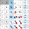 |
Fig. 6. For each galaxy highlighted in Fig. 4, we present the reconstructed HST/F160W source-plane image, the corresponding observed HST/F160W image, the MUSE [O II] pseudo narrowband, the LOS velocity map and best-fitting GalPaK3D model, as well as P–V diagrams extracted from both the observed and model datacubes. The MUSE PSF FWHM is indicated by the hatched circle. The sequence of grey rectangles marks the 1 arcsec-wide slit used to extract the P–V diagrams. |
Before modelling the TFR, we assess the consistency between structural parameters derived from the [O II] datacubes and those obtained from broadband continuum imaging, finding good overall agreement. The median misalignment between the photometric and kinematic PA is 6°, and the median absolute deviation in log(Re) is 0.14 dex, with a modest systematic offset of −0.09 dex in [O II] relative to the single-Sérsic broadband estimate. Finally, we find that a substantial fraction of galaxies have [O II] Sérsic indices close to the imposed lower bound of 0.5, yielding both a median value and a median absolute deviation of 0.6 for this parameter.
6.2. Velocity and mass definitions
In the following, we model the TFR as
 (8)
(8)
where M represents either the stellar or the baryonic mass (in M⊙) and v is the circular velocity at 1.8 or 2Re (in km s−1). These radii are selected to match the velocity definitions adopted in local reference TFRs, and probe the outer, approximately flat region of the RCs.
Baryonic masses were obtained by adding a cold gas component, estimated from scaling relations, to the stellar masses. Molecular gas masses (Mgas, mol) follow the scaling relations of Tacconi et al. (2020, their Tab. 2b). For the atomic gas, we used predictions from the NEUTRALUNIVERSEMACHINE empirical model (Guo et al. 2023), which predicts the evolution of atomic and molecular gas based on observational constraints (including the HI-stellar mass relation at z ∼ 1 from Chowdhury et al. 2022) and the UNIVERSEMACHINE (Behroozi et al. 2019) model for galaxy formation. Specifically, we adopted their best-fit relation between HI depletion timescale τHI and stellar mass at z ∼ 15, and used it to infer the median HI mass log MHI, MS(M★). We further accounted for the dependence of HI mass on offset from the SFMS using log(MHI/MHI, MS) = λlog(SFR/SFRMS) with λ ≈ 0.4. The inferred HI mass was then multiplied by 1.33 to include helium (e.g. McGaugh 2012).
The inferred atomic gas fraction, defined as fgas, at = 1.33MHI/Mbar, ranges between < 1% and 77% (5th–95th percentiles), with a median of 22%. For the molecular gas fraction, defined as fgas, mol = Mgas, mol/Mbar, the corresponding range is 13 − 53%, with a median of 34%.
6.3. Fitting procedure and robustness tests
We adopted a Bayesian approach and used the MCMC sampler emcee (Foreman-Mackey et al. 2013) to obtain the posterior distributions of the model parameters. The fit follows an orthogonal maximum-likelihood approach (e.g. Lelli et al. 2019, Appendix A), assuming a constant Gaussian intrinsic scatter orthogonal to the best-fit relation (σ⊥, int) and accounting for independent uncertainties in velocity and mass. Velocity errors were taken as the posterior standard deviation from our kinematic fits, while stellar masses were assigned a uniform uncertainty of ±0.15 dex to capture modelling uncertainties, for example those related to the magnification, SFH, stellar evolution, nebular emission and dust attenuation assumptions (∼0.1 dex, Pacifici et al. 2023), which is larger than the median observational error reported by BAGPIPES (0.06 dex). Similarly, baryonic masses were assigned a uniform uncertainty of ±0.2 dex. Given the limited mass range of our sample, we fixed the slope to local reference values in our fiducial analysis, and fitted only for the zero point and intrinsic scatter orthogonal to the relation assuming broad uniform priors. MCMC sampling was run with 20 walkers over 10 000 steps, including a burn-in phase of 2000 steps.
Investigations of TFR evolution depend on the adopted velocity definition, the choice of local reference and sample selection. In our fiducial analysis, we used v1.8 for the sTFR and compared our results to Reyes et al. (2011)6. For the bTFR, we used v2.0 = vc(2Re) and compared to Lelli et al. (2019). In both cases, we retained only rotationally supported galaxies (v/σ0 > 1) with well-constrained velocities (Δv/v < 30%). We also performed fits with a free slope to verify that the local slopes remain compatible with our data. Finally, to evaluate the robustness of our results, we repeated the analysis, varying the velocity definition (at 1.8 or 2Re), the rotational-support criterion (v/σ0 > 1 or v/σ0 > 2), and the adopted local reference (Reyes et al. 2011 or Ristea et al. 2024).
7. Evolution of the TFR since z ∼ 1
7.1. The TFR at z ∼ 1
We now turn to the sTFR and bTFR of our sample, shown in Fig. 7 together with the fiducial best-fitting relations and their posterior distributions. The corresponding parameters are listed in Table 3. When the slope is allowed to vary freely, the recovered slopes for both relations are consistent with local reference values. For the sTFR, we obtain  , consistent with the range asTFR = 3.6 − 3.9 commonly reported in local studies (Reyes et al. 2011; Lapi et al. 2018; Ristea et al. 2024) and in most high-redshift analyses (Sharma et al. 2024, and references therein). A notable exception is the significantly steeper slope (asTFR = 5.21 ± 0.18) found by Marasco et al. (2025) for a nearby sample spanning M★ = 108 − 11 M⊙. As discussed in Appendix D, their sTFR bends around M★ ∼ 1010 M⊙ and steepens towards lower masses. For the bTFR, we measured
  , consistent with the 3.14 ± 0.08 slope from Lelli et al. (2019).
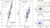 |
Fig. 7. sTFR (left) and bTFR (middle) for our sample. Solid blue and purple lines show the best-fit relations from our fiducial analyses, which adopt fixed slopes from the local references of Reyes et al. (2011) (sTFR) and Lelli et al. (2019) (bTFR), shown in black. Galaxies excluded from the fit (see text) are shown as open grey symbols. The top-right and bottom-right panels display the posterior distributions of these parameters for the sTFR and bTFR, respectively, with contours enclosing 39%, 86%, and 99% of the samples. For the sTFR, filled contours correspond to the fiducial analysis, while open contours show results obtained when varying the sample selection (in green), or the velocity definition and adopted reference slope (in orange). |
TFR best-fit parameters.
Given this overall consistency with local slopes, we adopted these reference values in our fiducial analysis and fitted only for the zero point and intrinsic scatter. For the sTFR, we fixed the slope to the Reyes et al. (2011) value because (i) it was calibrated over M★ = 109 − 11 M⊙, matching the projected mass range of our sample by z ≈ 0, and (ii) it agrees with other determinations over a similar range (Lapi et al. 2018; Ristea et al. 2024) as well as with our own data. This yields a zero point  , with an intrinsic orthogonal scatter of
  . For the bTFR, adopting the Lelli et al. (2019) slope results in
  and
and  . Relative to the corresponding local relations, the inferred zero point offsets are
  and
and  along the stellar mass axis. We now use our results to examine the evolution of the sTFR and bTFR zero points in the remainder of this section. We remind that our bTFR relies on cold gas scaling relations applied to the sTFR and is therefore more indirect and subject to larger uncertainties, particularly at the low-mass end.
7.2. Evolution of the sTFR
In Fig. 8, we compare our sTFR results to intermediate and high-redshift measurements of rotation-dominated galaxies, many of which were compiled and reprocessed by Turner et al. (2017), adopting a slope fixed to that of Reyes et al. (2011). We used the total velocities  from their compilation, where the rotation velocity v⊥ was extracted at 1.3 − 2Re depending on the sample, and σint is the beam-smearing corrected velocity dispersion. This definition includes a pressure-support correction similar to that of Dalcanton & Stilp (2010) and is therefore directly comparable to the circular velocities used in this work,
  . For a representative galaxy with M★ = 109 M⊙, v⊥(1.8Re) = 70 km/s and σint ≈ σ0 = 30 km/s, we find log(vtot)−log(v1.8) = + 0.03 dex, corresponding to a ≃ − 0.1 dex shift along the stellar-mass axis in the sTFR.
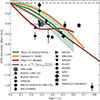 |
Fig. 8. Evolution of the sTFR zero point with redshift, shown relative to the local calibration of Reyes et al. (2011) along the stellar mass axis. Also plotted are predictions from the EAGLE hydrodynamical simulation (presented in Tiley et al. 2016, the shaded region indicates the rms dispersion of simulated SFGs), the Dutton et al. (2011) semi-analytical model, the empirical model of Übler et al. (2017) along with their measurements on the KMOS3D sample, and the evolution attributed to cosmology. For comparison, we include a compilation of literature measurements (see text), many of which were assembled and reprocessed by Turner et al. (2017). Horizontal error bars indicate the redshift range of our sample while vertical error bars show the fitting uncertainties for each sample. |
The comparison samples include Pelliccia et al. (2017, HR-COSMOS, z ∼ 0.9), Harrison et al. (2017, KROSS, z ∼ 0.9), Epinat et al. (2012, MASSIV, z ∼ 1.2), Simons et al. (2016, SIGMA, z ∼ 1.5 and z ∼ 2.3), Cresci et al. (2009, SINS, z ∼ 2.0), Straatman et al. (2017, ZFIRE, z ∼ 2.2) and Turner et al. (2017, KDS, z ∼ 3.5). We exclude the DYNAMO (Green et al. 2014), MKS (Swinbank et al. 2017), and AMAZE (Gnerucci et al. 2011) samples, which are not directly comparable to our analysis. As discussed by Turner et al. (2017), the DYNAMO sample is selected for high specific SFRs and gas fractions; the MKS velocities are not corrected for beam smearing, which may lead to underestimated velocities at fixed stellar mass; and the AMAZE sample, as reprocessed by Turner et al. (2017), contains only five galaxies.
We additionally include the offsets reported by Übler et al. (2017, KMOS3D, z ∼ 0.9 and z ∼ 2.3), whose velocities are measured at maximum (≈2.2Rd), and those reported by Danhaive et al.; Danhaive et al. (2025; 2026, FRESCO/CONGRESS, z ∼ 5), with velocities measured at Re. We also fitted and derived sTFR offsets for the Abril-Melgarejo et al. (2021, MAGIC, z ∼ 0.7), Mercier et al. (2022, MAGIC, z ∼ 0.7) and Pelliccia et al. (2019, ORELSE, z ∼ 0.9) samples, which probe galaxies across environments of varying density and measure velocities at 2.2Rd. Finally, we fitted the sTFR offset of the Girard et al. (2020, KLASS, z ∼ 1.3) and Mancera Piña et al. (2026, KROSS+KMOS3D, z ∼ 0.9) samples, whose velocities are extracted in the flat part of their RCs (≳2Re). For comparison, we also show predictions from the EAGLE hydrodynamical simulation (presented in Tiley et al. 2016), the semi-analytical model of Dutton et al. (2011), the empirical model presented in Übler et al. (2017), and the expected evolution due to the redshift dependence of ![Mathematical equation: $ \left[H(z)\sqrt{\Delta_c(z)}\right]^{-1} $](/articles/aa/full_html/2026/05/aa59953-26/aa59953-26-eq57.gif) , where Δc(z) is the DM halo overdensity following Bryan & Norman (1998).
, where Δc(z) is the DM halo overdensity following Bryan & Norman (1998).
Our measurements are qualitatively consistent with predicted evolutions, indicating lower stellar masses at fixed velocity compared to the local relation. Quantitatively, the observed offset is most compatible with the empirical model of Übler et al. (2017), the EAGLE SFGs, and the expected evolution driven by the redshift dependence of halo-defining quantities. Our results are in agreement with other z ∼ 1 studies targeting a similar mass range (Mercier et al. 2022) or more massive galaxies (M★ ∼ 1010 M⊙; Übler et al. 2017; Pelliccia et al. 2017; Harrison et al. 2017; Epinat et al. 2012), once pressure support is taken into account. This is interesting considering the various systematic differences between those samples in terms of selection (e.g. definition of rotational support, probed stellar mass range), velocity measurement (e.g. velocity definition, 2D/3D modelling, pressure-support correction) and stellar mass measurement (e.g. stellar population assumptions). While we do not engage in an extensive comparison of these systematics, we stress that our analysis relies on 3D forward modelling of the full datacubes, whereas most comparison studies model 2D velocity fields (Übler et al. 2017; Harrison et al. 2017; Epinat et al. 2012) or 2D slit spectra (Pelliccia et al. 2017, 2019). We also note differences in the adopted criteria for rotational support, with Übler et al. (2017) imposing a much stricter threshold of  , compared to v⊥/σ0 > 1 in other samples reprocessed by Turner et al. (2017) and the criterion v1.8/σ0 > 1 adopted here. We find that our conclusions are relatively robust to these choices: adopting v2.0 and the local reference of Ristea et al. (2024) reduces the inferred evolution to
  , while imposing a stricter rotational-support criterion (v1.8/σ0 > 2) increases it to
  , at ∼1σ of the fiducial offset. Finally, we infer an orthogonal intrinsic scatter of 0.10 − 0.12 dex, significantly above local estimates (0.02 − 0.08 dex). Following Mancera Piña et al. (2026), we tested whether the increased scatter could arise from underestimated velocity uncertainties. We therefore inflated the errors along the velocity axis until the fitted intrinsic scatter matched local estimates. This requires adding ≃0.10 dex in quadrature to the velocity uncertainties: an increase that would imply modelling or methodological errors (e.g. the impact of non-circular motions, see Dado et al. 2026) beyond the recovery performance quantified in Sect. 4 (≃0.05 dex). We also verified that inflating errors in this way does not significantly affect the inferred zero point. Since the 0.15 dex uncertainty on stellar mass is already intended to capture magnification and typical SED-modelling errors (Pacifici et al. 2023), and given the homogeneity of our sample, explaining the excess intrinsic scatter through additional stellar-mass errors would also imply unknown modelling or methodological uncertainties at the ≃0.35 dex level.
To interpret the observed evolution of the sTFR, we relate it to the evolution of DM haloes. Assuming a spherical top-hat collapse, halo masses are defined as Mvir(z) = 4πrvir3(z)Δc(z)ρc(z)/3, where rvir(z) is the virial radius, within which the mean halo density is Δc(z) times the critical density of the Universe, ρc(z) = 3H(z)2/(8πG). The evolution of the sTFR can be written (Dutton et al. 2011; Mancera Piña et al. 2026)
![Mathematical equation: $$ \begin{aligned} \left[ \frac{M_\star (z)}{M_\star (0)} \right] =&\left[ \frac{H(z) \sqrt{\Delta _c(z)}}{H_0 \sqrt{\Delta _c(0)}}\right]^{-1} \nonumber \\&\left[ \frac{f_M(M_{\rm vir}, z)}{f_M(M_{\rm vir}, 0)} \right] \left[ \frac{f_V(M_{\rm vir}, z)}{f_V(M_{\rm vir}, 0)} \right]^{-3} \left[ \frac{v_{1.8}(z)}{v_{1.8}(0)} \right]^3, \end{aligned} $$](/articles/aa/full_html/2026/05/aa59953-26/aa59953-26-eq61.gif) (9)
(9)
where fV = v1.8/vvir with vvir = vvir(Mvir, z) the virial velocity, and fM = M★/Mvir.
The first term on the right-hand side of Eq. (9) evolves by −0.34 dex between z = 0 and z ∼ 1, accounting for most of the observed offset. This implies that the product fMfV−3 evolves only weakly over this redshift interval. Our conclusions differ from those of Mancera Piña et al. (2026), who argue for significant evolution through both the sTFR slope and zero point. Given that their z ∼ 1 slope is consistent with ours, the discrepancy in the inferred slope evolution appears to stem from their adopted local reference relation (Marasco et al. 2025), which bends and steepens towards the low-mass end. Within the overlapping mass range, however, it is broadly consistent with other z ≈ 0 determinations (Reyes et al. 2011; Lapi et al. 2018; Ristea et al. 2024) and with our results (see Appendix D). The remaining difference would therefore concern the zero point. In principle, this offset could reflect systematic shifts in stellar mass estimates driven by differences in stellar population synthesis models, dust attenuation prescriptions, or assumed SFHs. However, this explanation appears insufficient, given the homogeneous SED treatment adopted by Mancera Piña et al. (2026) relative to Marasco et al. (2025), the agreement between dynamically and photometrically inferred stellar masses reported by Marasco et al. (2025), and, on the other hand, the body of previous studies that infer significant zero point evolution. A severe systematic offset in velocity also seems unlikely, pointing instead to sample selection effects or other unaccounted methodological biases.
We now consider whether the predicted or observed evolutions of fM and fV are quantitatively compatible with our results. The ratio fV is expected to increase modestly with cosmic time (Dutton et al. 2010, 2011), reflecting the predicted increase in DM halo concentration by ≃ + 0.1 − 0.2 dex since z ∼ 1 (Dutton & Macciò 2014; Anbajagane et al. 2022; Sorini et al. 2025) for galaxies with M★ ∼ 109 M⊙. While this evolution remains poorly constrained observationally, initial tests of the concentration - halo mass relation at z ∼ 1 are broadly consistent with predictions (Bouché et al. 2022; Sharma et al. 2022; Ciocan et al. 2026). Neglecting baryonic effects and assuming an NFW halo (Navarro et al. 1997), this implies an evolution of fV−3 of ≃ − 0.1 dex since z ∼ 1 (Dutton et al. 2010, their Eq. 8). On the other hand, abundance-matching models (e.g. Behroozi et al. 2019; Girelli et al. 2020) predict an increase in the stellar mass fraction fM of ≃ + 0.3 dex since z ∼ 1. Recent observational results from the COSMOS-Web survey, based on abundance matching (Shuntov et al. 2025) or halo occupation distribution (Paquereau et al. 2025) approaches, tend to show even weaker evolution (or even hints at a larger fM at z ∼ 1). Taken together, those expectations are consistent with a nearly constant or weakly evolving fMfV−3, and a sTFR evolution dominated by the redshift dependence of halo-defining quantities since z ∼ 1.
Fig. 8 suggests that this conclusion is supported by other samples around cosmic noon (Simons et al. 2016; Cresci et al. 2009; Straatman et al. 2017; Turner et al. 2017). ALMA and JWST now offer the opportunity to probe this picture at much earlier cosmic times. Dynamically cold discs are now identified at z ≳ 4 using ALMA observations of the [C II] λ158 μm line (e.g. Rizzo et al. 2020, 2021; Fraternali et al. 2021; Herrera-Camus et al. 2022) and, using JWST/NIRCam grism spectroscopy targeting Hα emission, Danhaive et al. (2025) report that roughly 40% of their sample of SFGs appear rotationally supported at z ∼ 5. Using the same sample, Danhaive et al. (2026) further suggest that the sTFR may already be emerging at that epoch. They report a comparable intrinsic scatter (0.49 dex in stellar mass), and measure an offset of −1.6 dex at z ∼ 5 for galaxies with M★ > 108 M⊙, of which −1.0 dex can be explained by the redshift dependence of ![Mathematical equation: $ \left[H(z)\sqrt{\Delta_c(z)}\right]^{-1} $](/articles/aa/full_html/2026/05/aa59953-26/aa59953-26-eq62.gif) .
.
7.3. Evolution of the bTFR
In Fig. 9, we compare our bTFR measurements with predictions from the SIMBA hydrodynamical simulation (Glowacki et al. 2021), the semi-analytical model of Dutton et al. (2011), and the empirical model of Übler et al. (2017), including the offsets they report at z ∼ 0.9 and z ∼ 2.3 relative to the local relation of Lelli et al. (2016b). We also show the expected evolution driven solely by the redshift dependence of ![Mathematical equation: $ \left[H(z)\sqrt{\Delta_c(z)}\right]^{-1} $](/articles/aa/full_html/2026/05/aa59953-26/aa59953-26-eq63.gif) , following the same interpretation developed for the sTFR around Eq. (9).
, following the same interpretation developed for the sTFR around Eq. (9).
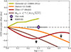 |
Fig. 9. Evolution of the bTFR zero point with redshift, shown relative to the local calibration of Lelli et al. (2019) along the stellar mass axis. Also plotted are predictions from the SIMBA hydrodynamical simulation (Glowacki et al. 2021), the Dutton et al. (2011) semi-analytical model, the empirical model of Übler et al. (2017) along with their measurements on the KMOS3D sample. Horizontal error bars indicate the redshift range of our sample while vertical error bars show the fitting uncertainties for each sample. |
Taking into account both the statistical and systematic uncertainties of our sample, as well as the ±0.16 dex statistical uncertainty in the local bTFR zero point (Lelli et al. 2019), we find that our results are consistent with the predictions of the Dutton et al. (2011) model. When considered together with our sTFR results (where the observed evolution is relatively more pronounced) our findings may indicate a stronger evolution of the cold gas fraction since z ∼ 1 relative to their model. In contrast to the SIMBA predictions of Glowacki et al. (2021), we do not observe an increase in baryonic mass at fixed circular velocity. We note, however, that in their analysis this trend appears only when adopting velocities measured in the flat part of the RCs, and is not seen for other velocity metrics based on linewidths. We further note that their simulated sample includes low-mass galaxies (Mbar < 1010 M⊙) that deviate from the bTFR towards lower baryonic masses at fixed velocity (see their Fig. 6), a behaviour that is not present in our sample and may indicate systematic differences related to sample selection. Finally, our results differ from those of Übler et al. (2017), who report a moderate evolution of the bTFR since z ∼ 1, despite the good agreement between the two studies regarding the sTFR evolution. We attribute this discrepancy to the non-negligible contribution of atomic gas to the overall baryonic mass budget in our galaxies (rather than to the mass budget within the velocity measurement radius as assumed in Übler et al. 2017) based on recent empirical constraints (Chowdhury et al. 2022). Notably, both studies rely on similar scaling relations to estimate molecular gas masses.
Investigating the scatter of the bTFR is particularly informative, as the remarkable tightness of this relation in the local Universe suggests that it may be more fundamental than other dynamical scaling relations, such as the sTFR or the Fall relation (McGaugh 2012; Lelli et al. 2016b, 2019; Hua et al. 2025). We find that the intrinsic orthogonal scatter of our bTFR is approximately three times larger (in dex) than that measured locally by Lelli et al. (2019, 0.05 dex). Disentangling the origin of this increased scatter is, however, challenging. In addition to the larger measurement uncertainties and the enhanced contribution of non-circular motions expected at high redshift (especially when using ionised gas tracers, see Rizzo et al. 2024; Kohandel et al. 2024), this likely reflects the limited precision of our cold gas mass estimates, which rely on scaling relations and constitute a limitation of our analysis. As for the sTFR, we note that one would need to inflate the velocity uncertainties by 0.15 dex in quadrature to recover the intrinsic scatter measured locally, and that doing so does not significantly affect the inferred bTFR zero point.
Since the early findings of Puech et al. (2010), who already reported no significant evolution of the bTFR at z ∼ 0.6, observational constraints on the bTFR from distant galaxies remain scarce, particularly those based on direct measurements of cold gas masses and kinematics. We highlight the first HI-based studies by Ponomareva et al. (2021) (0 ≤ z ≤ 0.081), Gogate et al. (2023) (z ∼ 0.2), and Jarvis et al. (2025) (z ∼ 0.35), as well as the CO-based bTFR study of Topal et al. (2018) (0.05 ≤ z ≤ 0.3), all of which report no significant evolution of the bTFR over their respective redshift ranges. Gogate et al. (2023) further examine environmental effects and find no measurable dependence of the bTFR on cluster environment. Studies of the sTFR based on ionised gas tracers similarly report little to no environmental dependence at higher redshift, provided that the samples being compared are defined and analysed homogeneously (Pelliccia et al. 2019; Mercier et al. 2022, the latter contrasting the significant offsets reported by Abril-Melgarejo et al. 2021 and attributing them to methodological biases). Upcoming measurements of HI masses and linewidths from the Square Kilometre Array (SKA) and its pathfinders (Staveley-Smith & Oosterloo 2015) will be key in extending bTFR constraints to earlier cosmic times.
8. Conclusions
In this work, we presented an extension of the 3D forward-modelling tool GalPaK3D, developed to recover the intrinsic morphology and kinematics of strongly lensed galaxies. We validated this extension using mock lensed datacubes and demonstrated its performance relative to direct image-plane fitting. We then applied this methodology to a sample of 116 star-forming main-sequence galaxies at z ∼ 1, drawn from the MUSE Atlas of Lensing Clusters and magnified by Hubble Frontier Fields clusters. For each galaxy, we forward-modelled the [O II] emission to recover its kinematics, derived stellar population properties through SED modelling, and reconstructed the intrinsic morphology in the source plane.
Using mock lensed datacubes representative of our sample, we showed that the intrinsic morpho-kinematic properties of strongly lensed SFGs can be reliably recovered provided they are rotation dominated (v1.8/σ0 > 1) and satisfy  , with α ≃ 1. We note that the recovered parameters exhibit relative uncertainties comparable to those obtained in the unlensed case at similar S/Neff. We find that this approach is significantly more robust, particularly for morphological parameters and velocity dispersion, with improvements by factors ≃2 − 4 in relative errors, than methods that neglect differential magnification, even for moderate magnifications (μ < 6).
Restricting our analysis to 95 galaxies that are rotationally supported (v1.8/σ0 > 1) and have well-constrained velocities (Δv1.8/v1.8 < 30%), we find no evidence for an evolution in the slopes of either the sTFR or bTFR. Adopting fixed slopes from local reference relations for the sTFR (Reyes et al. 2011) and for the bTFR (Lelli et al. 2019), we measure a significant evolution of the sTFR zero point,  in stellar mass, while the bTFR zero point remains consistent with its local value,
  . In both cases, we find an intrinsic scatter that is larger than in the local Universe, although it remains difficult to determine whether this reflects genuine physical evolution or unaccounted observational uncertainties.
For the sTFR, our measurements are in good agreement with other z ∼ 1 studies (Übler et al. 2017; Pelliccia et al. 2017; Harrison et al. 2017; Epinat et al. 2012; Mercier et al. 2022), once pressure support is taken into account. We tested the robustness of our results by varying the velocity definition and the adopted reference relation on the one hand, and the criterion to identify rotationally supported galaxies on the other hand. These choices affected the inferred zero point offset at the ∼1σ level but do not alter our conclusions. We also find consistency with the empirical model of Übler et al. (2017), predictions from EAGLE simulated SFGs, and the evolution expected from the redshift dependence of halo-defining quantities.
Interpreting the evolution of the sTFR in the framework of DM halo growth, we conclude that the observed offset is largely driven by the evolution of the factor ![Mathematical equation: $ \left[H(z)\sqrt{\Delta_c(z)}\right]^{-1} $](/articles/aa/full_html/2026/05/aa59953-26/aa59953-26-eq67.gif) . This implies that the product fMfV−3, where fM = M★/Mvir and fV = vc/vvir, has evolved only weakly since z ∼ 1. This behaviour is consistent with current predictions for the evolution of the stellar-to-halo mass ratio and halo concentrations over the past ∼8 Gyr. We highlight, however, a contrasting interpretation by Mancera Piña et al. (2026), who infer a significant evolution of fMfV−3 through both the sTFR slope and zero point. We attribute the discrepancy in slope evolution to differences in the adopted local reference relations, considering that our best-fit sTFR slope at z ∼ 1 (
. This implies that the product fMfV−3, where fM = M★/Mvir and fV = vc/vvir, has evolved only weakly since z ∼ 1. This behaviour is consistent with current predictions for the evolution of the stellar-to-halo mass ratio and halo concentrations over the past ∼8 Gyr. We highlight, however, a contrasting interpretation by Mancera Piña et al. (2026), who infer a significant evolution of fMfV−3 through both the sTFR slope and zero point. We attribute the discrepancy in slope evolution to differences in the adopted local reference relations, considering that our best-fit sTFR slope at z ∼ 1 ( ) is compatible with theirs (
 ). The remaining zero point offset is difficult to attribute to systematic shifts in stellar masses or circular velocities arising from measurement or modelling choices, and may instead point to residual sample selection or methodological biases.
Finally, the absence of detectable evolution in the bTFR zero point suggests that the increasing contribution of cold gas mass at higher redshift fully compensates the evolution observed in the stellar component alone. The increased intrinsic scatter of the bTFR probably highlights the current limitations imposed by indirect cold gas mass estimates based on scaling relations. Future high-redshift HI surveys will be valuable to further constrain the physical origin and cosmic evolution of both the sTFR and bTFR, providing direct measurements of the cold gas reservoir as well as homogeneous kinematics measurements that probe the outermost regions.
Data availability
The catalog described in Table E.1 is available at the CDS via https://cdsarc.cds.unistra.fr/viz-bin/cat/J/A+A/709/A120.
Acknowledgments
This work utilises gravitational lensing models produced by PIs Natarajan & Kneib (CATS), Sharon, Keeton, Diego, and the GLAFIC group. This lens modeling was partially funded by the HST Frontier Fields programme conducted by STScI. STScI is operated by the Association of Universities for Research in Astronomy, Inc. under NASA contract NAS 5-26555. The lens models were obtained from the Mikulski Archive for Space Telescopes (MAST). Beyond those already cited, this work makes use of the following open-source Python libraries: Astropy (Astropy Collaboration 2022), NumPy (Harris et al. 2020), matplotlib (Hunter 2007), MPDAF (Piqueras et al. 2017), SciPy (Virtanen et al. 2020) and corner (Foreman-Mackey 2016). NB and BC acknowledge support from the ANR DARK grant (ANR-22-CE31-0006). This research has made use of the VizieR catalogue access tool, CDS, Strasbourg Astronomical Observatory, France (DOI: 10.26093/cds/vizier). AJ acknowledges his fiancée, Adélaïde Claeyssens, for her support and patience during the preparation of this manuscript.
References
- Abril-Melgarejo, V., Epinat, B., Mercier, W., et al. 2021, A&A, 647, A152 [NASA ADS] [CrossRef] [EDP Sciences] [Google Scholar]
- Amorisco, N. C., & Bertin, G. 2010, A&A, 519, A47 [Google Scholar]
- Anbajagane, D., Evrard, A. E., & Farahi, A. 2022, MNRAS, 509, 3441 [Google Scholar]
- Astropy Collaboration (Price-Whelan, A. M., et al.) 2022, ApJ, 935, 167 [NASA ADS] [CrossRef] [Google Scholar]
- Bacon, R., Accardo, M., Adjali, L., et al. 2010, SPIE Conf. Ser., 7735, 773508 [Google Scholar]
- Bacon, R., Conseil, S., Mary, D., et al. 2017, A&A, 608, A1 [NASA ADS] [CrossRef] [EDP Sciences] [Google Scholar]
- Bartelmann, M., & Schneider, P. 2001, Phys. Rep., 340, 291 [Google Scholar]
- Beauchesne, B., Clément, B., Hibon, P., et al. 2024, MNRAS, 527, 3246 [Google Scholar]
- Behroozi, P., Wechsler, R. H., Hearin, A. P., & Conroy, C. 2019, MNRAS, 488, 3143 [NASA ADS] [CrossRef] [Google Scholar]
- Bell, E. F., & de Jong, R. S. 2001, ApJ, 550, 212 [Google Scholar]
- Boogaard, L. A., Brinchmann, J., Bouché, N., et al. 2018, A&A, 619, A27 [NASA ADS] [CrossRef] [EDP Sciences] [Google Scholar]
- Bosma, A. 1978, Ph.D. Thesis, University of Groningen, The Netherlands [Google Scholar]
- Bouché, N., Carfantan, H., Schroetter, I., Michel-Dansac, L., & Contini, T. 2015a, Astrophysics Source Code Library [record ascl:1501.014] [Google Scholar]
- Bouché, N. F., Carfantan, H., Schroetter, I., Michel-Dansac, L., & Contini, T. 2015b, AJ, 150, 92 [CrossRef] [Google Scholar]
- Bouché, N. F., Genel, S., Pellissier, A., et al. 2021, A&A, 654, A49 [NASA ADS] [CrossRef] [EDP Sciences] [Google Scholar]
- Bouché, N. F., Bera, S., Krajnović, D., et al. 2022, A&A, 658, A76 [NASA ADS] [CrossRef] [EDP Sciences] [Google Scholar]
- Brammer, G. B., Marchesini, D., Labbé, I., et al. 2016, ApJS, 226, 6 [NASA ADS] [CrossRef] [Google Scholar]
- Bruzual, G., & Charlot, S. 2003, MNRAS, 344, 1000 [NASA ADS] [CrossRef] [Google Scholar]
- Bryan, G. L., & Norman, M. L. 1998, ApJ, 495, 80 [NASA ADS] [CrossRef] [Google Scholar]
- Buchner, J. 2016, Astrophysics Source Code Library [record ascl:1606.005] [Google Scholar]
- Bullock, J. S., & Boylan-Kolchin, M. 2017, ARA&A, 55, 343 [Google Scholar]
- Burkert, A., Förster Schreiber, N. M., Genzel, R., et al. 2016, ApJ, 826, 214 [Google Scholar]
- Calzetti, D., Armus, L., Bohlin, R. C., et al. 2000, ApJ, 533, 682 [NASA ADS] [CrossRef] [Google Scholar]
- Cappellari, M. 2025, MNRAS, 544, 1432 [Google Scholar]
- Cappellari, M., McDermid, R. M., Alatalo, K., et al. 2013, MNRAS, 432, 1862 [NASA ADS] [CrossRef] [Google Scholar]
- Carnall, A. C., McLure, R. J., Dunlop, J. S., & Davé, R. 2018, MNRAS, 480, 4379 [Google Scholar]
- Carnall, A. C., McLure, R. J., Dunlop, J. S., et al. 2019, MNRAS, 490, 417 [Google Scholar]
- Chabrier, G. 2003, PASP, 115, 763 [Google Scholar]
- Chase, H., Dado, D., Harborne, K. E., & Oman, K. A. 2025, ArXiv e-prints [arXiv:2511.23106] [Google Scholar]
- Chirivì, G., Yıldırım, A., Suyu, S. H., & Halkola, A. 2020, A&A, 643, A135 [EDP Sciences] [Google Scholar]
- Chowdhury, A., Kanekar, N., & Chengalur, J. N. 2022, ApJ, 941, L6 [NASA ADS] [CrossRef] [Google Scholar]
- Ciocan, B. I., Bouché, N. F., Fensch, J., et al. 2026, A&A, 708, A112 [Google Scholar]
- Claeyssens, A., Richard, J., Blaizot, J., et al. 2022, A&A, 666, A78 [NASA ADS] [CrossRef] [EDP Sciences] [Google Scholar]
- Contini, T., Epinat, B., Bouché, N., et al. 2016, A&A, 591, A49 [NASA ADS] [CrossRef] [EDP Sciences] [Google Scholar]
- Courteau, S. 1997, AJ, 114, 2402 [Google Scholar]
- Cresci, G., Hicks, E. K. S., Genzel, R., et al. 2009, ApJ, 697, 115 [Google Scholar]
- Dado, D., Oman, K. A., Harborne, K. E., et al. 2026, MNRAS, 547, stag356 [Google Scholar]
- Dalcanton, J. J., & Stilp, A. M. 2010, ApJ, 721, 547 [NASA ADS] [CrossRef] [Google Scholar]
- Danhaive, A. L., Tacchella, S., Übler, H., et al. 2025, MNRAS, 543, 3249 [Google Scholar]
- Danhaive, A. L., Tacchella, S., Bunker, A. J., et al. 2026, MNRAS, 546, stag119 [Google Scholar]
- Di Teodoro, E. M., & Fraternali, F. 2015, MNRAS, 451, 3021 [Google Scholar]
- Di Teodoro, E. M., Grillo, C., Fraternali, F., et al. 2018, MNRAS, 476, 804 [NASA ADS] [CrossRef] [Google Scholar]
- Dutton, A. A., & Macciò, A. V. 2014, MNRAS, 441, 3359 [Google Scholar]
- Dutton, A. A., Conroy, C., van den Bosch, F. C., Prada, F., & More, S. 2010, MNRAS, 407, 2 [Google Scholar]
- Dutton, A. A., van den Bosch, F. C., Faber, S. M., et al. 2011, MNRAS, 410, 1660 [NASA ADS] [Google Scholar]
- Epinat, B. 2008, PhD Thesis, Université de Provence, France [Google Scholar]
- Epinat, B., Tasca, L., Amram, P., et al. 2012, A&A, 539, A92 [NASA ADS] [CrossRef] [EDP Sciences] [Google Scholar]
- Fall, S. M., & Efstathiou, G. 1980, MNRAS, 193, 189 [NASA ADS] [CrossRef] [Google Scholar]
- Famaey, B., & McGaugh, S. S. 2012, Liv. Rev. Relativ., 15, 10 [Google Scholar]
- Feroz, F., Hobson, M. P., & Bridges, M. 2009, MNRAS, 398, 1601 [NASA ADS] [CrossRef] [Google Scholar]
- Foreman-Mackey, D. 2016, J. Open Source Software, 1, 24 [NASA ADS] [CrossRef] [Google Scholar]
- Foreman-Mackey, D., Hogg, D. W., Lang, D., & Goodman, J. 2013, PASP, 125, 306 [Google Scholar]
- Förster Schreiber, N. M., & Wuyts, S. 2020, ARA&A, 58, 661 [Google Scholar]
- Förster Schreiber, N. M., Genzel, R., Lehnert, M. D., et al. 2006, ApJ, 645, 1062 [Google Scholar]
- Förster Schreiber, N. M., Renzini, A., Mancini, C., et al. 2018, ApJS, 238, 21 [Google Scholar]
- Fraternali, F., Karim, A., Magnelli, B., et al. 2021, A&A, 647, A194 [NASA ADS] [CrossRef] [EDP Sciences] [Google Scholar]
- Genzel, R., Förster Schreiber, N. M., Übler, H., et al. 2017, Nature, 543, 397 [Google Scholar]
- Genzel, R., Price, S. H., Übler, H., et al. 2020, ApJ, 902, 98 [NASA ADS] [CrossRef] [Google Scholar]
- Gilbank, D. G., Baldry, I. K., Balogh, M. L., Glazebrook, K., & Bower, R. G. 2010, MNRAS, 405, 2594 [NASA ADS] [Google Scholar]
- Ginsburg, A., Robitaille, T., & Beaumont, C. 2016, Astrophysics Source Code Library [record ascl:1608.010] [Google Scholar]
- Girard, M., Dessauges-Zavadsky, M., Schaerer, D., et al. 2018, A&A, 613, A72 [NASA ADS] [CrossRef] [EDP Sciences] [Google Scholar]
- Girard, M., Mason, C. A., Fontana, A., et al. 2020, MNRAS, 497, 173 [Google Scholar]
- Girelli, G., Pozzetti, L., Bolzonella, M., et al. 2020, A&A, 634, A135 [NASA ADS] [CrossRef] [EDP Sciences] [Google Scholar]
- Glowacki, M., Elson, E., & Davé, R. 2021, MNRAS, 507, 3267 [NASA ADS] [Google Scholar]
- Gnerucci, A., Marconi, A., Cresci, G., et al. 2011, A&A, 528, A88 [NASA ADS] [CrossRef] [EDP Sciences] [Google Scholar]
- Gogate, A. R., Verheijen, M. A. W., van der Hulst, J. M., & Jaffé, Y. L. 2023, MNRAS, 519, 4279 [Google Scholar]
- Green, A. W., Glazebrook, K., McGregor, P. J., et al. 2014, MNRAS, 437, 1070 [Google Scholar]
- Guérou, A., Krajnović, D., Epinat, B., et al. 2017, A&A, 608, A5 [Google Scholar]
- Guo, H., Wang, J., Jones, M. G., & Behroozi, P. 2023, ApJ, 955, 57 [NASA ADS] [CrossRef] [Google Scholar]
- Harris, C. R., Millman, K. J., van der Walt, S. J., et al. 2020, Nature, 585, 357 [NASA ADS] [CrossRef] [Google Scholar]
- Harrison, C. M., Johnson, H. L., Swinbank, A. M., et al. 2017, MNRAS, 467, 1965 [Google Scholar]
- Herrera-Camus, R., Förster Schreiber, N. M., Price, S. H., et al. 2022, A&A, 665, L8 [NASA ADS] [CrossRef] [EDP Sciences] [Google Scholar]
- Hua, Z., Lelli, F., Di Teodoro, E., McGaugh, S., & Schombert, J. 2025, A&A, 703, A223 [Google Scholar]
- Hunter, J. D. 2007, Comput. Sci. Eng., 9, 90 [NASA ADS] [CrossRef] [Google Scholar]
- Jarvis, M. J., Tudorache, M. N., Heywood, I., et al. 2025, MNRAS, 544, 193 [Google Scholar]
- Jones, T. A., Swinbank, A. M., Ellis, R. S., Richard, J., & Stark, D. P. 2010, MNRAS, 404, 1247 [NASA ADS] [Google Scholar]
- Jones, T., Ellis, R. S., Richard, J., & Jullo, E. 2013, ApJ, 765, 48 [NASA ADS] [CrossRef] [Google Scholar]
- Jullo, E., Kneib, J. P., Limousin, M., et al. 2007, New J. Phys., 9, 447 [Google Scholar]
- Kneib, J. P., Ellis, R. S., Smail, I., Couch, W. J., & Sharples, R. M. 1996, ApJ, 471, 643 [Google Scholar]
- Kohandel, M., Pallottini, A., Ferrara, A., et al. 2024, A&A, 685, A72 [NASA ADS] [CrossRef] [EDP Sciences] [Google Scholar]
- Kroupa, P. 2001, MNRAS, 322, 231 [NASA ADS] [CrossRef] [Google Scholar]
- Lagattuta, D. J., Richard, J., Bauer, F. E., et al. 2019, MNRAS, 485, 3738 [NASA ADS] [Google Scholar]
- Lang, P., Förster Schreiber, N. M., Genzel, R., et al. 2017, ApJ, 840, 92 [NASA ADS] [CrossRef] [Google Scholar]
- Lapi, A., Salucci, P., & Danese, L. 2018, ApJ, 859, 2 [Google Scholar]
- Lee, L. L., Förster Schreiber, N. M., Price, S. H., et al. 2025, ApJ, 978, 14 [Google Scholar]
- Leethochawalit, N., Jones, T. A., Ellis, R. S., et al. 2016, ApJ, 820, 84 [NASA ADS] [CrossRef] [Google Scholar]
- Leja, J., Carnall, A. C., Johnson, B. D., Conroy, C., & Speagle, J. S. 2019a, ApJ, 876, 3 [Google Scholar]
- Leja, J., Johnson, B. D., Conroy, C., et al. 2019b, ApJ, 877, 140 [NASA ADS] [CrossRef] [Google Scholar]
- Lelli, F., McGaugh, S. S., & Schombert, J. M. 2016a, AJ, 152, 157 [Google Scholar]
- Lelli, F., McGaugh, S. S., & Schombert, J. M. 2016b, ApJ, 816, L14 [Google Scholar]
- Lelli, F., McGaugh, S. S., Schombert, J. M., Desmond, H., & Katz, H. 2019, MNRAS, 484, 3267 [NASA ADS] [CrossRef] [Google Scholar]
- Lian, J., & Luo, L. 2024, ApJ, 960, L10 [Google Scholar]
- Liu, D., Förster Schreiber, N. M., Genzel, R., et al. 2023, ApJ, 942, 98 [NASA ADS] [CrossRef] [Google Scholar]
- Livermore, R. C., Jones, T. A., Richard, J., et al. 2015, MNRAS, 450, 1812 [Google Scholar]
- Lotz, J. M., Koekemoer, A., Coe, D., et al. 2017, ApJ, 837, 97 [Google Scholar]
- Madau, P., & Dickinson, M. 2014, ARA&A, 52, 415 [Google Scholar]
- Mahler, G., Richard, J., Clément, B., et al. 2018, MNRAS, 473, 663 [Google Scholar]
- Mancera Piña, P. E., Di Teodoro, E. M., Fall, S. M., et al. 2026, A&A, 705, A180 [Google Scholar]
- Marasco, A., Fall, S. M., Di Teodoro, E. M., & Mancera Piña, P. E. 2025, A&A, 695, L23 [NASA ADS] [CrossRef] [EDP Sciences] [Google Scholar]
- Mason, C. A., Treu, T., Fontana, A., et al. 2017, ApJ, 838, 14 [NASA ADS] [CrossRef] [Google Scholar]
- McGaugh, S. S. 2012, AJ, 143, 40 [Google Scholar]
- McGaugh, S. S., Schombert, J. M., Bothun, G. D., & de Blok, W. J. G. 2000, ApJ, 533, L99 [Google Scholar]
- McGaugh, S. S., Lelli, F., & Schombert, J. M. 2016, Phys. Rev. Lett., 117, 201101 [NASA ADS] [CrossRef] [Google Scholar]
- Mercier, W., Epinat, B., Contini, T., et al. 2022, A&A, 665, A54 [NASA ADS] [CrossRef] [EDP Sciences] [Google Scholar]
- Mo, H. J., Mao, S., & White, S. D. M. 1998, MNRAS, 295, 319 [Google Scholar]
- Muñoz López, C., Krajnović, D., Epinat, B., et al. 2024, A&A, 688, A75 [NASA ADS] [CrossRef] [EDP Sciences] [Google Scholar]
- Navarro, J. F., Frenk, C. S., & White, S. D. M. 1997, ApJ, 490, 493 [Google Scholar]
- Nedkova, K. V., Häußler, B., Marchesini, D., et al. 2021, MNRAS, 506, 928 [NASA ADS] [CrossRef] [Google Scholar]
- Neeleman, M., Prochaska, J. X., Kanekar, N., & Rafelski, M. 2020, Astrophysics Source Code Library [record ascl:2005.013] [Google Scholar]
- Neeleman, M., Novak, M., Venemans, B. P., et al. 2021, ApJ, 911, 141 [NASA ADS] [CrossRef] [Google Scholar]
- Nestor Shachar, A., Price, S. H., Förster Schreiber, N. M., et al. 2023, ApJ, 944, 78 [NASA ADS] [CrossRef] [Google Scholar]
- Pacifici, C., Iyer, K. G., Mobasher, B., et al. 2023, ApJ, 944, 141 [NASA ADS] [CrossRef] [Google Scholar]
- Paquereau, L., Laigle, C., McCracken, H. J., et al. 2025, A&A, 702, A163 [NASA ADS] [CrossRef] [EDP Sciences] [Google Scholar]
- Patrício, V., Richard, J., Carton, D., et al. 2018, MNRAS, 477, 18 [Google Scholar]
- Pelliccia, D., Tresse, L., Epinat, B., et al. 2017, A&A, 599, A25 [NASA ADS] [CrossRef] [EDP Sciences] [Google Scholar]
- Pelliccia, D., Lemaux, B. C., Tomczak, A. R., et al. 2019, MNRAS, 482, 3514 [Google Scholar]
- Persic, M., Salucci, P., & Stel, F. 1996, MNRAS, 281, 27 [Google Scholar]
- Piqueras, L., Conseil, S., Shepherd, M., et al. 2017, ArXiv e-prints [arXiv:1710.03554] [Google Scholar]
- Ponomareva, A. A., Mulaudzi, W., Maddox, N., et al. 2021, MNRAS, 508, 1195 [NASA ADS] [Google Scholar]
- Posti, L. 2022, Res Notes Am. Astron. Soc., 6, 233 [Google Scholar]
- Price, S. H., Shimizu, T. T., Genzel, R., et al. 2021, ApJ, 922, 143 [NASA ADS] [CrossRef] [Google Scholar]
- Puech, M., Hammer, F., Flores, H., et al. 2010, A&A, 510, A68 [NASA ADS] [CrossRef] [EDP Sciences] [Google Scholar]
- Puglisi, A., Dudzevičiūtė, U., Swinbank, M., et al. 2023, MNRAS, 524, 2814 [NASA ADS] [CrossRef] [Google Scholar]
- Reyes, R., Mandelbaum, R., Gunn, J. E., Pizagno, J., & Lackner, C. N. 2011, MNRAS, 417, 2347 [Google Scholar]
- Richard, J., Claeyssens, A., Lagattuta, D., et al. 2021, A&A, 646, A83 [EDP Sciences] [Google Scholar]
- Ristea, A., Cortese, L., Fraser-McKelvie, A., et al. 2024, MNRAS, 527, 7438 [Google Scholar]
- Rizzo, F., Vegetti, S., Fraternali, F., & Di Teodoro, E. 2018, MNRAS, 481, 5606 [Google Scholar]
- Rizzo, F., Vegetti, S., Powell, D., et al. 2020, Nature, 584, 201 [Google Scholar]
- Rizzo, F., Vegetti, S., Fraternali, F., Stacey, H. R., & Powell, D. 2021, MNRAS, 507, 3952 [NASA ADS] [CrossRef] [Google Scholar]
- Rizzo, F., Bacchini, C., Kohandel, M., et al. 2024, A&A, 689, A273 [NASA ADS] [CrossRef] [EDP Sciences] [Google Scholar]
- Rohatgi, A. 2010, WebPlotDigitizer [Google Scholar]
- Rubin, V. C., Ford, W. K., Jr, & Thonnard, N. 1978, ApJ, 225, L107 [Google Scholar]
- Sanders, R. H., & McGaugh, S. S. 2002, ARA&A, 40, 263 [NASA ADS] [CrossRef] [Google Scholar]
- Sérsic, J. L. 1963, Bol. Asociacion Argentina Astron La Plata Argentina, 6, 41 [Google Scholar]
- Sharma, G., Salucci, P., Harrison, C. M., van de Ven, G., & Lapi, A. 2021, MNRAS, 503, 1753 [CrossRef] [Google Scholar]
- Sharma, G., Salucci, P., & van de Ven, G. 2022, A&A, 659, A40 [NASA ADS] [CrossRef] [EDP Sciences] [Google Scholar]
- Sharma, G., Upadhyaya, V., Salucci, P., & Desai, S. 2024, A&A, 689, A318 [Google Scholar]
- Shipley, H. V., Lange-Vagle, D., Marchesini, D., et al. 2018, ApJS, 235, 14 [Google Scholar]
- Shuntov, M., Ilbert, O., Toft, S., et al. 2025, A&A, 695, A20 [NASA ADS] [CrossRef] [EDP Sciences] [Google Scholar]
- Simons, R. C., Kassin, S. A., Trump, J. R., et al. 2016, ApJ, 830, 14 [Google Scholar]
- Simons, R. C., Kassin, S. A., Snyder, G. F., et al. 2019, ApJ, 874, 59 [Google Scholar]
- Sorini, D., Bose, S., Pakmor, R., et al. 2025, MNRAS, 536, 728 [Google Scholar]
- Staveley-Smith, L., & Oosterloo, T. 2015, Advancing Astrophysics with the Square Kilometre Array (AASKA14), 167 [Google Scholar]
- Straatman, C. M. S., Glazebrook, K., Kacprzak, G. G., et al. 2017, ApJ, 839, 57 [Google Scholar]
- Straatman, C. M. S., van der Wel, A., van Houdt, J., et al. 2022, ApJ, 928, 126 [Google Scholar]
- Ströbele, S., La Penna, P., Arsenault, R., et al. 2012, SPIE Conf. Ser., 8447, 844737 [Google Scholar]
- Swinbank, A. M., Papadopoulos, P. P., Cox, P., et al. 2011, ApJ, 742, 11 [NASA ADS] [CrossRef] [Google Scholar]
- Swinbank, A. M., Harrison, C. M., Trayford, J., et al. 2017, MNRAS, 467, 3140 [NASA ADS] [Google Scholar]
- Tacconi, L. J., Genzel, R., & Sternberg, A. 2020, ARA&A, 58, 157 [NASA ADS] [CrossRef] [Google Scholar]
- Tiley, A. L., Stott, J. P., Swinbank, A. M., et al. 2016, MNRAS, 460, 103 [Google Scholar]
- Tiley, A. L., Bureau, M., Cortese, L., et al. 2019, MNRAS, 482, 2166 [Google Scholar]
- Topal, S., Bureau, M., Tiley, A. L., Davis, T. A., & Torii, K. 2018, MNRAS, 479, 3319 [Google Scholar]
- Torres-Flores, S., Epinat, B., Amram, P., Plana, H., & Mendes de Oliveira, C. 2011, MNRAS, 416, 1936 [Google Scholar]
- Tsukui, T., Wisnioski, E., Bland-Hawthorn, J., & Freeman, K. 2025, MNRAS, 540, 3493 [Google Scholar]
- Tully, R. B., & Fisher, J. R. 1977, A&A, 54, 661 [NASA ADS] [Google Scholar]
- Turner, O. J., Harrison, C. M., Cirasuolo, M., et al. 2017, ArXiv e-prints [arXiv:1711.03604] [Google Scholar]
- Übler, H., Förster Schreiber, N. M., Genzel, R., et al. 2017, ApJ, 842, 121 [Google Scholar]
- Übler, H., Genzel, R., Wisnioski, E., et al. 2019, ApJ, 880, 48 [Google Scholar]
- Übler, H., Förster Schreiber, N. M., van der Wel, A., et al. 2024, MNRAS, 527, 9206 [Google Scholar]
- van der Wel, A., Franx, M., van Dokkum, P. G., et al. 2014, ApJ, 788, 28 [Google Scholar]
- Virtanen, P., Gommers, R., Oliphant, T. E., et al. 2020, Nat. Methods, 17, 261 [Google Scholar]
- Weaver, J. R., Davidzon, I., Toft, S., et al. 2023, A&A, 677, A184 [NASA ADS] [CrossRef] [EDP Sciences] [Google Scholar]
- Weilbacher, P. M., Palsa, R., Streicher, O., et al. 2020, A&A, 641, A28 [NASA ADS] [CrossRef] [EDP Sciences] [Google Scholar]
- Wisnioski, E., Mendel, J. T., Leaman, R., et al. 2025, MNRAS, 544, 2777 [Google Scholar]
- Yttergren, M., Knudsen, K. K., Molina, J., et al. 2025, MNRAS, 543, 3103 [Google Scholar]
As an example, Posti (2022) demonstrates that treating (blank field) velocity measurements along a RC as independent leads to biased parameter estimates and underestimated errors. Building on this approach, Chase et al. (2025) show that accounting for correlations between RC datapoints is critical to determine whether RCs from the SPARC database (Lelli et al. 2016a) statistically favour cored or cuspy DM haloes.
The impact of PSF FWHM errors is discussed in Sect. 4.4 of Bouché et al. (2015b).
For v1.8 and σ0, we suppose α = 0.8 based on the coefficient derived by Bouché et al. (2015b) for vmax.
Using the WebPlotDigitizer (Rohatgi 2010), we digitised the best-fit average relation between log τHI ≡ log⟨MHI⟩−⟨logSFR⟩ and ⟨log M★⟩ from their Fig. 16, and converted it to a median relation assuming lognormal HI masses and the reported 0.8 dex scatter in log τHI.
To allow a meaningful comparison with the literature samples compiled by Turner et al. (2017), we adopted their local reference relation derived from the Reyes et al. (2011) dataset.
Appendix A: Summary of the MUSE observations and ancillary datasets
Tab. A.1 summarises the MUSE observations and ancillary datasets used in this work (Sect. 2). Note that the MACS0416 north (N) and south (S) pointings have been analysed separately.
Summary of the MUSE observations and ancillary datasets.
Appendix B: Properties of the mock sample
Fig. B.1 compares the properties of the mock sample (Sect. 4) with those of the kinematic sample (Sect. 5). After applying similar selection cuts, the distributions of most properties in the mocks closely match the kinematic sample, except the highest circular velocities and lowest velocity dispersions, which are both under-represented in the mock sample.
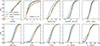 |
Fig. B.1. Properties of the mock sample compared to the kinematic sample. From top left to bottom right, we show the cumulative distribution functions (CDFs) of redshift, magnification, stellar mass, SFR, effective radius, apparent size-to-PSF ratio, S/N in the brightest spaxel, effective S/N, circular velocity at 1.8Re and velocity dispersion floor. The rotation-dominated (v1.8/σ0 > 1) subset of the kinematic sample with well-constrained velocities (Δv1.8/v1.8 < 30%) is shown in solid orange. A further restriction to μ < 6, applied to match the magnification range of the mock sample for a fair comparison of the magnification CDFs, is indicated by the dash-dotted orange line. The parent mock sample appears as a dashed blue line, while the mock subsample satisfying selection criteria similar to the kinematic sample (S/Neff > 10, |
Appendix C: The impact of cluster mass modelling errors
The GalPaK3D Strong Lensing Extension described in Sect. 3 uses deflection maps derived from a lens model to account for the lensing distortions. Therefore, the inferred morpho-kinematic properties are affected by lens model errors over which our extension does not marginalise. In this Appendix, we assess the impact of those errors by comparing the circular velocities obtained with the fiducial model from R21 to those derived using an average model constructed from five publicly available models7: the R21 model together with models produced by PIs Sharon, Keeton, Diego, and the GLAFIC group (as described in Lotz et al. 2017). Instead of directly averaging magnification values (which are highly non-linear), we constructed this average model by re-gridding the available maps (deflection along both axes, potential, convergence and projected shear along both axes) to the same reference frame and averaging them.
From our fiducial analysis, we retained 95 galaxies that are rotationally supported (v1.8/σ0 > 1) and have well-constrained velocities (Δv1.8/v1.8 < 30%). We removed 24 galaxies which were included as lenses in at least one lens model, and extracted the morpho-kinematics of the remaining galaxies using the same modelling assumptions and priors as for the fiducial lens model.
Fig. C.1 compares the circular velocities obtained with the average and R21 lens models and shows overall excellent agreement. We find a median absolute deviation of 0.003 dex, with a single outlier at 0.4 dex. This galaxy (ID4517) lies close to the critical lines of Abell 370 (μ = 30–60), where cluster mass models are known to be particularly sensitive to modelling uncertainties. Overall, this comparison indicates that the circular velocities derived in this work are robust to uncertainties in the cluster mass modelling.
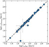 |
Fig. C.1. Comparison of circular velocities derived using the R21 lens model adopted in this work with those obtained from an average lens model constructed from publicly available models including R21. |
Appendix D: Comparison with the sTFR slope evolution reported by Mancera Piña et al. (2026)
In this Appendix, we compare the stellar masses and circular velocities measured in this work with those reported by Mancera Piña et al. (2026, hereafter MP26). MP26 find moderate evidence for a shallower sTFR slope at z ∼ 1 compared to the z ≈ 0 relation of Marasco et al. (2025), implying a shallower fM − M★ relation if fV is assumed independent of stellar mass and redshift. Fig. D.1 shows the sTFR from MP26 and our sample at z ∼ 1, together with z ≈ 0 reference relations (Reyes et al. 2011; Marasco et al. 2025; Lapi et al. 2018, polynomial fit) limited to the stellar mass range of the corresponding data. The Marasco et al. (2025) sample spans M★ = 108 − 11 M⊙ and is consistent with previous results for log(vc/[km s−1]) > 2.15. At lower velocities, the sTFR steepens, indicating lower stellar masses at fixed circular velocity. While this break has previously been reported around log(vc/[km s−1]) ≃ 1.95 (e.g. McGaugh et al. 2000; Torres-Flores et al. 2011), in this sample the departure occurs at higher velocities. Within the overlapping mass range, we do not observe a departure in slope between our results, MP26, and previous z ≈ 0 determinations, but mostly a difference in zero point.
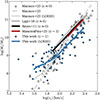 |
Fig. D.1. Comparison of the sTFR at z ∼ 1 from MP26 and this work, alongside z ≈ 0 reference relations (Reyes et al. 2011; Lapi et al. 2018; Marasco et al. 2025). Our sample and that of Marasco et al. (2025) are shown as blue and grey symbols, respectively, with LOESS-smoothed curves (Cappellari et al. 2013) highlighting the trends. The unbroken power-law sTFR from Marasco et al. (2025) is shown as a dashed grey line. |
Appendix E: Catalogue
Description of the columns included in the catalogue associated with this paper.
All Tables
Main parameters of our kinematic model, together with their adopted priors or fixed values.
Parameters of our SED model, together with their adopted priors or fixed values.
Description of the columns included in the catalogue associated with this paper.
All Figures
|
Fig. 1. Schematic view of the lensing configuration and coordinate frames. The observed image-frame coordinates rimg − r0img are mapped to source-frame coordinates rsrc − r0src via the lens equation |
| In the text | |
|
Fig. 2. Comparison of the relative errors in the inferred properties, defined as δp/p = (pfit − ptrue)/ptrue, for a kinematic model fitted either directly in the image frame (left column) or in the source frame using the GalPaK3D Strong Lensing Extension (right column). Each row shows the error density distribution for a given property, restricted to the rotation-dominated subsample of mock galaxies (v1.8/σ0 > 1). The effective radius is corrected a posteriori by the magnification when fitted in the image plane. The PA error is relative to PAtrue = 130°, as in Bouché et al. (2015b). Dashed lines show the empirical relation |
| In the text | |
|
Fig. 3. Same as Fig. 2, but additionally restricted to the subsample of mock galaxies satisfying μ > 3. |
| In the text | |
|
Fig. 4. S/N of the brightest [O II] spaxel against the apparent size-to-PSF ratio. The hatched grey region marks the parameter space excluded by our selection. Red symbols mark 6 galaxies chosen to showcase the range of apparent sizes and S/N in Fig. 6. Open symbols mark galaxies that are either dispersion-dominated (v1.8/σ0 ≤ 1) or have poorly constrained velocities (Δv1.8/v1.8 ≥ 30%), where Δv1.8 is the posterior standard deviation. The background hexagonal bins illustrate the fraction of rotation-dominated (v1.8/σ0 > 1) mock galaxies with a robust velocity recovery ( |
| In the text | |
|
Fig. 5. General sample properties. The panels show the distributions of redshift (top left) and magnification (bottom left), together with the locations of the galaxies in the M★–SFR (middle) and M★–Re (right) planes. Effective radii are corrected to rest-frame 5000 Å following Eqs. 1 and 2 of van der Wel et al. (2014), expressed relative to the size–mass relation of Nedkova et al. (2021) (interpolated with redshift), and scaled to z = 1. Similarly, SFRs are expressed relative to the star-forming main sequence of Boogaard et al. (2018), adjusted to the redshift and stellar mass of each galaxy, and normalised to z = 1. The shaded regions indicate the ±1σ (dark grey) and ±2σ (light grey) scatter around the corresponding relations. Open symbols and histogram segments mark galaxies that are either dispersion-dominated (v1.8/σ0 ≤ 1) or have poorly constrained velocities (Δv1.8/v1.8 ≥ 30%), where Δv1.8 is the posterior standard deviation. |
| In the text | |
|
Fig. 6. For each galaxy highlighted in Fig. 4, we present the reconstructed HST/F160W source-plane image, the corresponding observed HST/F160W image, the MUSE [O II] pseudo narrowband, the LOS velocity map and best-fitting GalPaK3D model, as well as P–V diagrams extracted from both the observed and model datacubes. The MUSE PSF FWHM is indicated by the hatched circle. The sequence of grey rectangles marks the 1 arcsec-wide slit used to extract the P–V diagrams. |
| In the text | |
|
Fig. 7. sTFR (left) and bTFR (middle) for our sample. Solid blue and purple lines show the best-fit relations from our fiducial analyses, which adopt fixed slopes from the local references of Reyes et al. (2011) (sTFR) and Lelli et al. (2019) (bTFR), shown in black. Galaxies excluded from the fit (see text) are shown as open grey symbols. The top-right and bottom-right panels display the posterior distributions of these parameters for the sTFR and bTFR, respectively, with contours enclosing 39%, 86%, and 99% of the samples. For the sTFR, filled contours correspond to the fiducial analysis, while open contours show results obtained when varying the sample selection (in green), or the velocity definition and adopted reference slope (in orange). |
| In the text | |
|
Fig. 8. Evolution of the sTFR zero point with redshift, shown relative to the local calibration of Reyes et al. (2011) along the stellar mass axis. Also plotted are predictions from the EAGLE hydrodynamical simulation (presented in Tiley et al. 2016, the shaded region indicates the rms dispersion of simulated SFGs), the Dutton et al. (2011) semi-analytical model, the empirical model of Übler et al. (2017) along with their measurements on the KMOS3D sample, and the evolution attributed to cosmology. For comparison, we include a compilation of literature measurements (see text), many of which were assembled and reprocessed by Turner et al. (2017). Horizontal error bars indicate the redshift range of our sample while vertical error bars show the fitting uncertainties for each sample. |
| In the text | |
|
Fig. 9. Evolution of the bTFR zero point with redshift, shown relative to the local calibration of Lelli et al. (2019) along the stellar mass axis. Also plotted are predictions from the SIMBA hydrodynamical simulation (Glowacki et al. 2021), the Dutton et al. (2011) semi-analytical model, the empirical model of Übler et al. (2017) along with their measurements on the KMOS3D sample. Horizontal error bars indicate the redshift range of our sample while vertical error bars show the fitting uncertainties for each sample. |
| In the text | |
|
Fig. B.1. Properties of the mock sample compared to the kinematic sample. From top left to bottom right, we show the cumulative distribution functions (CDFs) of redshift, magnification, stellar mass, SFR, effective radius, apparent size-to-PSF ratio, S/N in the brightest spaxel, effective S/N, circular velocity at 1.8Re and velocity dispersion floor. The rotation-dominated (v1.8/σ0 > 1) subset of the kinematic sample with well-constrained velocities (Δv1.8/v1.8 < 30%) is shown in solid orange. A further restriction to μ < 6, applied to match the magnification range of the mock sample for a fair comparison of the magnification CDFs, is indicated by the dash-dotted orange line. The parent mock sample appears as a dashed blue line, while the mock subsample satisfying selection criteria similar to the kinematic sample (S/Neff > 10, |
| In the text | |
|
Fig. C.1. Comparison of circular velocities derived using the R21 lens model adopted in this work with those obtained from an average lens model constructed from publicly available models including R21. |
| In the text | |
|
Fig. D.1. Comparison of the sTFR at z ∼ 1 from MP26 and this work, alongside z ≈ 0 reference relations (Reyes et al. 2011; Lapi et al. 2018; Marasco et al. 2025). Our sample and that of Marasco et al. (2025) are shown as blue and grey symbols, respectively, with LOESS-smoothed curves (Cappellari et al. 2013) highlighting the trends. The unbroken power-law sTFR from Marasco et al. (2025) is shown as a dashed grey line. |
| In the text | |
Current usage metrics show cumulative count of Article Views (full-text article views including HTML views, PDF and ePub downloads, according to the available data) and Abstracts Views on Vision4Press platform.
Data correspond to usage on the plateform after 2015. The current usage metrics is available 48-96 hours after online publication and is updated daily on week days.
Initial download of the metrics may take a while.