| Issue |
A&A
Volume 709, May 2026
|
|
|---|---|---|
| Article Number | A239 | |
| Number of page(s) | 15 | |
| Section | Numerical methods and codes | |
| DOI | https://doi.org/10.1051/0004-6361/202659116 | |
| Published online | 19 May 2026 | |
Comparative analysis of missing data imputation methods for CSST survey: Impact on photometric redshift estimation performance
1
Shanghai Key Lab for Astrophysics, Shanghai Normal University,
Shanghai
200234,
China
2
Center for Astronomy and Space Sciences, China Three Gorges University,
Yichang
443000,
PR China
3
South-Western Institute for Astronomy Research, Yunnan University,
Kunming
650500,
China
4
Department of Astronomy, School of Physics,Peking University,
Beijing
100871,
China
5
Changchun Institute of Optics, Fine Mechanics and Physics, Chinese Academy of Sciences,
Changchun
130033,
China
6
University Observatory, Faculty of Physics, Ludwig-Maximilians-Universität,
Scheinerstr. 1,
81679
Munich, Germany
7
National Astronomical Observatories, Chinese Academy of Sciences,
20A Datun Road, Chaoyang District,
Beijing
100101,
PR China
8
Purple Mountain Observatory, Chinese Academy of Sciences,
Nanjing
210023,
China
9
School of Physics and Astronomy, Sun Yat-sen University,
Zhuhai
519082,
PR China
10
Shanghai Astronomical Observatory, Chinese Academy of Sciences,
80 Nandan Road,
Shanghai
200030,
PR China
11
CSST Science Center for the Guangdong-Hong Kong-Macau Greater Bay Area,
Zhuhai
519082,
PR China
12
School of Physics and Electronics, Hunan Normal University,
36 Lushan Road,
Changsha
410081,
China
13
Computer Network Information Center, Chinese Academy of Sciences,
2 East Kexueyuan South Road, Haidian District,
Beijing
100083,
PR China
14
Center for Astrophysics and Great Bay Center of National Astronomical Data Center, Guangzhou University,
Guangzhou,
Guangdong
510006,
PR China
15
Faculty of Information Engineering and Automation, Kunming University of Science and Technology,
No.727 Jingming South Road,
Kunming
650500,
PR China
16
School of Astronomy and Space Science, University of Chinese Academy of Sciences,
Beijing
101408,
PR China
17
Key Laboratory of Space Astronomy and Technology, National Astronomical Observatories, Chinese Academy of Sciences,
Beijing
100101,
China
★ Corresponding author: This email address is being protected from spambots. You need JavaScript enabled to view it.
Received:
25
January
2026
Accepted:
10
April
2026
Abstract
Improving the accuracy of photometric redshifts (photo-z) is essential for reliable statistical studies of cosmology and galaxy evolution. However, missing photometric bands are a common observational challenge that can significantly degrade photo-z estimation accuracy. In this work, we present a systematic evaluation of data imputation methods aimed at improving photo-z performance. We benchmark a range of representative machine learning and deep learning architectures, identifying k-nearest neighbors (KNN) and the attentionbased SAITS model as the leading performers. These models are then applied to China Space Station Survey Telescope mock data to assess their performance under realistic observational conditions. Our results show that KNN yields the highest accuracy under idealized missing completely at random (MCAR) conditions with complete training sets, whereas robustness tests reveal that SAITS significantly outperforms KNN when training data are incomplete or when applied to realistic mixed-mechanism scenarios. We find that domain consistency between training and testing missingness patterns is a prerequisite for optimal performance, highlighting the risks of domain shift in supervised regression tasks. Furthermore, our analysis demonstrates that while general imputation models are highly effective for MCAR and missing at random data, they are detrimental when applied to missing not at random data arising from flux limits, as statistical models fail to capture the physical information inherent in these nondetection. Consequently, we advocate for more sophisticated architectures capable of disentangling stochastic missingness from physical nondetection to address these distinct mechanisms individually.
Key words: methods: data analysis / methods: statistical / catalogs / galaxies: distances and redshifts / galaxies: photometry
© The Authors 2026
 Open Access article, published by EDP Sciences, under the terms of the Creative Commons Attribution License (https://creativecommons.org/licenses/by/4.0), which permits unrestricted use, distribution, and reproduction in any medium, provided the original work is properly cited.
This article is published in open access under the Subscribe to Open model. This email address is being protected from spambots. You need JavaScript enabled to view it. to support open access publication.
1 Introduction
Handling missing data is a common challenge in almost all fields of data analysis and has been extensively studied for decades (Little & Rubin 2019). Astronomical research is no exception, especially with regard to multiband photometric data. Missing values originate from diverse sources, ranging from poor observing conditions and limitation of instruments to the nondetection of faint sources and artifacts introduced when crossmatching surveys of different depths and coverage. Consequently, the prevalence of such incomplete data presents a significant challenge to reliable model fitting and hinders advanced scientific inference.
Three primary strategies are commonly used to address missing photometric data. The first and simplest is the case-wise deletion, which excludes any source with missing values from the sample. However, this approach has several drawbacks. First, it directly conflicts with the goal of maximizing the scientific utility of large astronomical surveys, as it inevitably reduces the sample size. Second, it risks introducing significant sample selection bias if the pattern of the missing data is not completely random.
The second strategy is to retain and flag missing values. This allows the algorithm with an inherent capability of handling missing data to proceed without explicit data imputation. For example, spectral energy distribution (SED) fitting algorithms (Brammer et al. 2008; Ilbert et al. 2006; Bolzonella et al. 2000) for photometric redshift (photo-z) can be configured to omit missing data points during χ2 minimization, while tree-based methods, such as random forest (RF) and boosting algorithms, can manage missing values intrinsically. However, the lack of complete information inevitably degrades the accuracy of downstream inferences such as photo-z regression. Furthermore, this strategy severely limits method selection, as many standard machine learning (ML) and deep learning (DL) models require complete numerical inputs. Similarly, traditional classification methods relying on color indices, used for star-galaxy separation or quasar selection (Schindler et al. 2017), fail if even a single necessary photometric band is unavailable.
The third and most sophisticated strategy is data imputation (Agarwal 2013). This technique estimates missing values from observed correlations, typically using statistical models or ML algorithms. By reconstructing a complete dataset, successful imputation can significantly increase the effective sample size available for scientific analysis. Consequently, developing a robust imputation algorithm capable of generating reliable estimates represents the most promising approach for maximizing dataset utility and minimizing sample selection bias.
Traditional statistical methods for data imputation often rely on models with relatively simple distribution assumptions and need to be reengineered and validated for different data types, thereby limiting their universal application. In contrast, ML and DL methods are data-driven, offering a superior capacity to capture complex high-dimensional data structures without predefined distributional forms and making them far more versatile and widely applicable across diverse datasets. As AI techniques have shown powerful data mining ability on big data in recent years, several studies have begun to explore ML and DL for astronomical data imputation.
An effective imputation algorithm must not only predict missing values with high precision but also preserve the underlying relationships between features (photometric data, colors, etc.) and the target labels (redshifts, object classification, etc.) after data completion. In the context of classification, Keerin & Boongoen (2022) applied two variant imputation methods based on k-nearest neighbor imputation (KNNimpute; Ma et al. 2020) and local least squares imputation (LLSimpute; Wang et al. 2019) separately for the classification of transient events. The Euclid PHZ pipeline adopted the KNN algorithm (Cover & Hart 1967) for data imputation before star-galaxy classification (Euclid Collaboration 2025). Regarding photo-z improvement, Luken et al. (2021) compared conventional ML methods (KNN and MICE; Van Buuren 2000) with a DL-based generative adversarial network (GAIN; Yoon et al. 2018) using a relatively small ATLAS dataset of approximately 1300 objects and found that MICE achieved the best performance. However, DL architectures are typically more complex than ML methods and generally require substantially larger training sets to avoid overfitting and to learn robust feature representations. Consequently, a sample of this size may limit the effectiveness of the DL model and may not provide a fully representative benchmark for comparing DL-and ML-based approaches. Luo et al. (2024) implemented GAIN on a large CSST simulation dataset and demonstrated its superior performance. Chartab et al. (2023) used the RF model to predict the magnitude of drop bands in their datasets; however, as their main goal was to apply information theory to reduce redundancy in band selection for optimal parameter prediction, they did not perform an extensive validation of the imputation itself. La Torre et al. (2024) constructed an self-organizing map likelihood from complete training data to infer the color of galaxies with missing data, thereby maximizing the data utility to improve the statistical accuracy of galaxy parameters. This strategy integrates DL with probabilistic techniques, relying on the assumption that the color distributions remain consistent between the training and test datasets.
Despite the development of various ML and DL methods for photometric data imputation, there is currently no consensus or clear guidance on which of these frameworks performs optimally for the unique characteristics of astronomical multiphotometry data. Given the significant advancements and robust performance of existing general-purpose ML and DL techniques, understanding their utility and limitations within our specific domain is warranted, rather than focusing on the creation of entirely new imputation frameworks. Consequently, a comprehensive and systematic evaluation of representative models spanning diverse architectural families is essential to elucidate the most effective strategies for addressing the challenges inherent to astronomical multiphotometry imputation. In this study, we systematically evaluate imputation performance by assessing the accuracy of photo-z estimations derived from a range of representative models.
Precise galaxy redshifts are fundamental for deriving key physical properties, such as mass and luminosity, and for studying the large-scale structure and evolution of the Universe (Conselice 2014; Tasca et al. 2009; Mo et al. 2010; Abdalla et al. 2011). The gold standard for accuracy is the spectroscopic redshift, which is determined by the analysis of discrete spectral features (Cole et al. 2005; Percival et al. 2007; Carrasco Kind & Brunner 2013). However, this spectroscopic method is observationally expensive and often requires long exposure times to achieve an adequate signal-to-noise ratio (S/N; Salvato et al. 2019), making it impractical for very large samples. This limitation has necessitated the widespread adoption of photo-z as a less precise but far more efficient alternative (Koo 1985; Loh & Spillar 1986; Feldmann et al. 2006). By estimating redshifts from broad- and medium-band photometry, this technique is pivotal for modern multiband sky surveys, facilitating cosmological statistical studies on galaxy populations that are orders of magnitude larger than those accessible to spectroscopy. As the era of large-scale surveys ushers in unprecedented opportunities for precision cosmology, achieving scientific goals remains critically dependent on deriving high-precision photo-z. Such accuracy is a cornerstone for major ongoing missions, including the Dark Energy Camera Legacy Survey (DECaLS; Dey et al. 2019), the Vera C. Rubin Observatory’s Legacy Survey of Space and Time (LSST; LSST Science Collaboration 2009; Ivezić et al. 2019), and the Euclid mission (Laureijs et al. 2011), and essential for the forthcoming survey of the Chinese Space Station Survey Telescope (CSST; Zhan 2011; Cao et al. 2018b; CSST Collaboration 2026. In this paper, we use simulated data for the CSST survey to systematically evaluate and compare the performance of several imputation techniques in improving photo-z precision.
The remainder of this paper is organized as follows. In Section 2 we detail the simulation dataset and the methodology used to generate realistic missing data patterns. In Section 3 we introduce the suite of imputation models under consideration. Our core comparative analysis is presented in Section 4, where we systematically evaluate the models based on the resulting photo-z accuracy from EAZY (Brammer et al. 2008) and assess their stability to select optimal approaches. In Section 5, we apply the optimal methods to realistic missing data scenarios anticipated for CSST. Finally, in Section 6 we summarize our key findings and present the conclusions of this study.
2 Dataset and evaluation method
The CSST is a 2-meter space telescope designed to be co-orbital with the China Manned Space Station (CSST Collaboration 2026). Cumulative observations with the CSST Survey Camera are planned for approximately 7 years of the 10-year orbital period in order to obtain wide-field survey data of 7-band (NUV, u, g, r, i, z, and y) photometric imaging over a sky area of about 17 500 deg2. The survey will reach 5σ pointsource depths of approximately 26 AB mag in the g, r, and i bands, and 24.4-25.4 AB mag in the remaining bands. The ambitious scientific goals of CSST include probing the evolution of large-scale structures, constraining the nature of dark matter and dark energy, and investigating galaxy formation and evolution (Gong et al. 2019; Zhan 2021; Cao et al. 2022; Liu et al. 2023). As CSST is China’s first optical space telescope, the CSST pipeline team has developed comprehensive simulations to model the survey strategy and instrumental effects (Wei et al. 2026a; Ban et al. 2026; Wei et al. 2026b; Xian et al. 2026). These efforts are crucial for building the data processing pipeline and evaluating the scientific potentials of the current survey design.
Our evaluation is based on data from the CSST Cycle 6 survey simulation, which emulates a 1.53 deg2 observation centered at RA = 244.97° and Dec = 39.90°. The simulation is designed for high fidelity, incorporating both physical phenomena such as weak lensing and cosmic rays as well as instrumental effects such as the point spread function, dark current, bias, flatfielding, and various detector artifacts. The underlying galaxy population for this simulation is sourced from the comprehensive Jiutian cosmological simulation (Han et al. 2025), which provides ground-truth properties for objects down to a magnitude of 28 across redshift up to 2.0.
This simulation yields two primary, co-spatial catalogs. The first is the input catalog as ground truth, which contains the intrinsic properties of all sources and serves as our benchmark for training and evaluation. The second is the output photometry catalog, a Level 2 data product generated by running the official CSST pipeline on the simulated images. This catalog contains realistic photometry and, critically, inherits authentic data missing patterns from the observational and processing limitations. It therefore represents the incomplete dataset that our imputation methods must address.
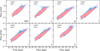 |
Fig. 1 Flux-error relations across bands. Input flux versus predicted flux errors (pink) and output catalog values (blue). |
2.1 Dataset construction
To establish a reliable ground truth for our analysis, we first constructed a complete dataset by selecting sources from the simulated CSST input catalog that possess valid photometric measurements across all seven bands. However, the input catalog only provides true, error-free magnitudes, whereas photometric uncertainties are unavoidable in actual observations. To produce a more realistic dataset suitable for downstream tasks such as SED fitting, which require flux errors, we implemented a magnitude error prediction model. This model leverages a RF algorithm, specifically trained to match the noise properties of the seven CSST bands. It operates by predicting realistic flux errors through a S/N matching mechanism, subsequently applying these errors to the true magnitudes in our complete input catalog.
The success of this error modeling is illustrated in Figure 1. We show the flux-error correlation for both the actual simulated pipeline output and our error-modeled input catalog. The close alignment between these two distributions shows that our model effectively reproduces the observational characteristics of the S/N, thus improving the realism of our complete dataset.
To systematically evaluate our imputation methods, we divide the complete dataset into distinct training, validation, and test sets. These divisions serve standard roles: the training set for model fitting, the validation set for hyperparameter tuning and preventing overfitting, and the test set for an unbiased final performance assessment. The details of these datasets are provided in Table 1.
Our experimental design for the training sets was twofold. First, to rigorously assess the impact of sample size on imputation performance, we constructed seven nested training sets of varying sizes. This nested approach ensures that each larger set is a superset of the smaller ones, thus isolating the effect of sample size from potential variations due to random sampling. Second, to investigate the influence of missingness in the training data itself, we introduced various missing data fractions into a specific 120 000 sample training set.
The test sets were specifically designed for a comprehensive and unbiased evaluation of the trained models under various conditions, and their corresponding validation sets were constructed with identical data missing patterns to ensure consistent evaluation during model development. We employed two schemes to introduce missing values under the missing completely at random (MCAR) assumption:
Scenario-based missingness: to assess model performance across a spectrum of common missingness patterns, we created test scenarios by selectively removing different combinations of photometric bands (e.g., one, two, or three bands per source).
Robustness-based missingness: to rigorously evaluate model robustness against varying degrees of data incompleteness, we applied a range of global missing rates (10, 20, or 30% of all photometric measurements) across the test set. The overall missing rate is defined as the total number of missing entries divided by the total number of possible entries in the dataset.
Following the imputation of missing magnitudes, a critical subsequent step is the generation of their corresponding flux errors. Since a missing magnitude inherently implies a missing error, we reapplied our previously described RF error model to the newly imputed magnitudes. This ensured that every entry in the completed catalog possesses both a magnitude and a realistic error, a prerequisite for photo-z estimation.
Our decision to employ the MCAR mechanism in this initial evaluation warrants explanation. While real observational data, such as CSST, will undoubtedly exhibit a complex mix of missing at random (MAR) and missing not at random (MNAR) components (e.g., nondetection of faint objects), our objective here is to establish a baseline performance comparison for imputation models within a controlled, idealized environment (Graham 2009; Demirtas 2018). Therefore, this initial analysis focuses exclusively on the MCAR case, with a comprehensive investigation into MAR and MNAR imputation deferred to future work.
Dataset partitioning and missing data settings.
2.2 Photo-z evaluation metrics
The ultimate application of an imputation method is its ability to improve downstream scientific results. Given that incomplete photometric data inherently degrade the reliability of photo-z determinations, we evaluate photo-z performance as our principal criterion for assessing imputation quality. We assess this performance using three key metrics.
The first metric is outlier fraction (fout). This metric identifies the fraction of sources with catastrophic photo-z. An object is considered an outlier if its estimated photo-z deviates significantly from its true redshift (zin), per the condition in
 (1)
(1)
The outlier fraction is  (Fotopoulou & Paltani 2018).
The second metric is the normalized median absolute deviation (σNMAD), which provides a robust measure of the photo-z precision (i.e., scatter). Following Brammer et al. (2008), it is defined as
 (2)
(2)
where ∆z = zphot — zin. The scaling factor of 1.48 makes this statistic comparable to the standard deviation of a normal distribution.
The final metric is the bias of the photo-z (bias), revealing whether redshifts are generally overestimated or underestimated. It was calculated as the median of the normalized residuals
 (3)
(3)
All photo-z were derived using the EAZY code (Brammer et al. 2008). Since different template-fitting codes tend to produce statistically comparable photo-z accuracy when run with the same configuration (Desprez et al. 2020), our findings using EAZY are expected to be broadly applicable. Our specific configuration utilized the “tweak_fsps_QSF_v12_v3” templates, which is based on the flexible stellar population synthesis (FSPS) code (Conroy et al. 2009), a standard ΛCDM cosmology (H0 = 70 km s−1 Mpc−1, Ωm = 0.3, Ωλ = 0.7), and default values for all other parameters.
3 Imputation methods
In selecting models for evaluation, we made a deliberate choice to prioritize methods representing fundamentally different underlying architectures. The overall accuracy and suitability of an imputation algorithm for a given dataset, particularly in complex domains such as astronomical multiphotometry, are primarily driven by its basic architectural paradigm rather than by minor variations or specific implementations within a single family of models. While iterative refinements and hyperparameter tuning can yield incremental improvements, significant performance differences are more likely to arise from the core structural approach (e.g., whether it is distance based, sequence aware, or attention based). Therefore, our selection criteria emphasized models built upon diverse architectural foundations to identify the most promising foundational approaches for this application.
3.1 Machine learning methods
KNN. The KNN algorithm (Cover & Hart 1967) is a distancebased learning method. For imputation, it identifies the k-nearest neighbors for a sample with missing values based on a distance metric (e.g., Euclidean distance) computed from the available observed features. The missing values are then estimated by a weighted average or the mean of the corresponding feature values from these neighbors. In this study, we implement KNN imputation using the KNNImputer module from the Scikit-learn library (Pedregosa et al. 2011).
RF. The RF (Breiman 2001) is an ensemble learning algorithm that performs regression by constructing a multitude of decision trees. For imputation, each tree is trained on a bootstrapped subsample of the data. To predict a missing value for a specific band, the RF model is trained to predict that band’s magnitude using the other observed bands as features. The final imputed value is the average of the predictions from all trees in the forest, which enhances robustness and reduces overfitting. The optimal number of trees is determined via k-fold cross-validation. The RF model we adopted is also implemented based on the Python interface of the Scikit-learn library (Pedregosa et al. 2011).
CatBoost. The CatBoost (Prokhorenkova et al. 2018; Veronika Dorogush et al. 2018) is a high-performance gradient boosting algorithm that builds decision trees sequentially, with each new tree correcting the errors of its predecessor. While primarily known for its sophisticated handling of categorical features, CatBoost also offers a powerful built-in mechanism for handling missing numerical values (via the nan_mode hyperparameter). This allows it to directly process and impute missing data without requiring external preprocessing steps, making it a highly efficient and integrated solution. The imputation is performed as part of the model’s internal training process when predicting a target variable. In terms of CatBoost, we directly employed its official Python package for our experiments1.
3.2 Deep learning methods
In recent years, DL has emerged as a powerful approach for missing value imputation. In this study, we utilize the PyPOTS Python package (Du et al. 2023b)2, a comprehensive library for partially observed time series data mining, especially for data imputation. We select a suite of state-of-the-art DL models designed for time-series data, also suitable for sequential data from the package, which are categorized by their underlying architectures below.
RNN-based. These models utilize recurrent neural networks to model sequential dependencies. We selected M-RNN (missing data recurrent neural network; Yoon et al. 2019) and BRITS (bidirectional recurrent imputation for time series; Cao et al. 2018a) for evaluation. M-RNN contains both an interpolation block and a subsequent imputation block, which are trained jointly. The model uses the interpolated values as an initial guess to improve the accuracy of the final imputation within the RNN structure. BRITS improves upon earlier RNN-based methods by treating imputed values as learnable variables within a bidirectional recurrent system. This allows the imputed values to be directly updated via backpropagation, leading to more accurate estimates compared to models such as M-RNN, where imputed values are treated as fixed constants during training updates. A notable drawback of many RNN-based models, however, is their autoregressive nature, which can lead to error accumulation (Venkatraman & Khaitan 2015).
GAN-based. These models frame imputation as a generative task, learning the underlying data distribution. We adopted US-GAN (unsupervised generative adversarial network; Miao et al. 2021) as our representative model. US-GAN adapts the standard GAN architecture for imputation, consisting of a Generator that learns to impute missing values and a Discriminator that attempts to distinguish between real and imputed data. The Generator, typically a Bidirectional RNN, is trained to minimize both an adversarial loss (to fool the Discriminator) and a reconstruction loss (to ensure consistency with observed data).
VAE-based. These models use a variational autoencoder framework to learn a low-dimensional latent representation of the data. We chose GP-VAE (Gaussian process variational autoencoder; Fortuin et al. 2020), a model specifically designed for time series with missing values. GP-VAE maps the incomplete highdimensional data to a continuous, low-dimensional latent space where there are no missing values. Crucially, it places a Gaussian process prior on this latent space, enforcing temporal smoothness and structure. The imputation is performed by encoding the incomplete data into this latent space and then decoding it back to the original data space, effectively reconstructing the missing values based on the learned temporal dynamics.
Self-attention-based. This category of models replaces traditional recurrence with attention mechanisms to capture dependencies across the entire data sequence. We included the original Transformer model (Vaswani et al. 2017), a recent variant iTrans-former (Liu et al. 2024), and SAITS (self-attention imputation for time series; Du et al. 2023a) as test models. The original Transformer model relies entirely on multihead self-attention to capture global dependencies between input and output. While designed for sequence transduction, its ability to relate different positions of a single sequence makes it applicable to imputation tasks. iTransformer inverts the standard Transformer architecture. It applies self-attention across different variables (i.e., photometric bands) at the same time step, treating the variables themselves as tokens. This is particularly well-suited for capturing the multivariate correlations inherent in photometric data. The SAITS model is specifically designed for imputation. It employs a joint-optimization objective that combines a standard imputation loss with a reconstruction loss. Its core consists of two diagonally masked self-attention blocks, which explicitly capture both temporal dependencies and feature correlations to effectively impute missing values in multivariate time series.
4 Experiments and results
To evaluate model performance, we used a fixed-size training set of 120 000 complete sources. The test sets were generated by randomly removing one, two, or three bands from each source. We assessed imputation quality using three standard metrics: mean absolute error (MAE), root mean square error (RMSE), and mean relative error (MRE). For a fair comparison, all models were trained with a batch size of 1024. This relatively large batch size was chosen due to the low dimensionality of the input data and the moderate model size, which allow efficient utilization of GPU memory. In practice, we found that larger batch sizes led to more stable training behavior. Hyperparameters were tuned using Optuna (Akiba et al. 2019), a Bayesian optimization framework, where the learning rate was treated as a tunable parameter to account for its coupling with batch size. An early stopping strategy was employed, halting training if the validation MAE did not improve for five consecutive epochs, all models converged within 100 epochs. All experiments were conducted on a single NVIDIA RTX 3090 GPU.
4.1 Imputation performance comparison
Table 2 reports the imputation performance of models on the three test datasets, as well as the accuracy of photo-z estimation for the imputed photometric datasets. Across all test scenarios, two models consistently emerged as the top performers: KNN and, to a close second, SAITS. Both models dramatically improve photo-z accuracy, approaching the performance achieved with the complete, original dataset. The impact is particularly striking in the most challenging case with three missing bands, where both methods reduce the photo-z outlier fraction by a factor of ten compared to the nonimputed baseline. The high fidelity of these imputations is visually confirmed in Figure 2, which compared the true versus imputed magnitudes. Figure 2a shows that KNN provides exceptionally accurate and unbiased imputations, while SAITS also performs very well (Figure 2b), it exhibits a slight systematic bias at the bright end, which we attribute to the relative scarcity of bright sources in the training data. To demonstrate the practical utility of our top-performing models, we also applied them to the more realistic output catalog, which incorporates observational noise and pipeline processing artifacts. For this purpose, the models were retrained using a subsample of the output catalog with complete data, enabling adaptation to additional observational features that are not present in the input catalog. Both KNN and SAITS again demonstrated robust performance. This is confirmed in Figure A.1 in Appendix A, which also shows the successful imputation of the output catalog even in the challenging scenario of three missing bands.
It is also noteworthy that while all tested ML methods performed well with a single dropped band, performance diverged as data sparsity increased. Tree-based methods (RF and CatBoost) exhibited a rapid decline in photometric accuracy as the number of missing bands rose, whereas KNN - a distance-based method - proved to be more robust. A similar trend was observed in DL models: RNN-based and GAN-based methods failed to maintain robustness as the number of missing bands increased, while transformer-based methods demonstrated significantly more stable performance.
Beyond imputation accuracy, computational cost is a critical practical consideration. Table 3 summarizes the parameter counts and training speeds for the DL models. Although transformer-based methods are more complex and contain more parameters than other DL architectures, their training time per epoch remains acceptable and is justified by the substantial improvement in photo-z accuracy. It is worth noting that the reported parameter counts vary across different drop-band scenarios, as the hyperparameters of each model are independently optimized using Optuna for each setting. Consequently, the resulting model complexity does not necessarily exhibit a monotonic relationship with the number of missing bands. This can be attributed to the stochastic nature of hyperparameter optimization in a high-dimensional search space.
Performance comparison of different methods on various drop bands.
Number of model parameters and training time per epoch for different numbers of missing bands.
4.2 Robustness analysis
Our previous experiments identified KNN and SAITS as the topperforming imputation models. However, realistic astronomical catalogs exhibit varying degrees of data sparsity, and relying on large, complete training sets is often impractical and prone to selection bias. Therefore, in this section, we conduct a rigorous evaluation of the robustness of these two leading models under variable conditions. Specifically, we assess their photo-z accuracy by systematically varying three key scenarios: the sparsity of the test set, the sample size of the training set, and the degree of incompleteness within the training data.
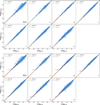 |
Fig. 2 Predicted versus true magnitudes for the test set with three missing photometric bands using the imputation models. Panel a: predicted versus true magnitudes (KNN). Panel b: same as (a) but for the SAITS model. We show the predicted values as a function of the true values. The dashed green line marks mag predict = mag true, and the red line shows the linear fit. |
4.2.1 Drop rate of test dataset analysis
First, we evaluated the models’ robustness to varying degrees of missing data in the test set. For this experiment, we retained the training dataset described in Section 4.1 but generated three separate test datasets with global missing rates of 10, 20 and 30%, as detailed in Table 1. For hyperparameter tuning, we utilized validation datasets with missing rates matching their corresponding test sets. Finally, each of these test sets was imputed using both the KNN and SAITS models.
The results presented in Figure 3 confirm that both models are highly effective in recovering photo-z accuracy. When trained on a complete dataset, KNN’s performance is consistently on par with and marginally better than that of SAITS across all missingness levels. The impact is substantial: even at a high missing fraction of 30%, KNN imputation reduces the photo-z outlier fraction by a factor of seven compared to the nonimputed baseline.
 |
Fig. 3 Photo-z quality metrics for the KNN and SAITS models for test sets with different missing data rates. Blue bars show the SED fitting on nonimputed data, and pink and purple bars show results after KNN and SAITS imputation, respectively. |
4.2.2 Training sample size analysis
To evaluate how the training sample size influences imputation performance, we trained KNN and SAITS on seven distinct datasets ranging from 5000 to 120 000 samples (see Table 1). These models were then evaluated against a fixed test set containing a global missing fraction of 10%.
The results reveal distinct performance curves for the two models (Figure 4). For large training sets (≥90 000 samples), both models achieve excellent and comparable performance, with photo-z outlier fractions around 1.5%. As the training sample size decreases, however, KNN demonstrates superior data efficiency. Its performance degrades gracefully, with the outlier fraction remaining a low 1.7% even with only 5000 training samples. In contrast, SAITS’s performance degrades more sharply once the training sample size drops below 90 000, reaching an outlier fraction of 2.19% with a 5000 sample set. This is attributable to the inherent data hunger of DL models; the parameter-heavy Transformer architecture struggles to generalize from small training sets, leading to suboptimal performance compared to the simpler distance-based KNN. This demonstrates that when a complete training set is available, KNN is not only more accurate but also significantly more data-efficient than SAITS, maintaining high performance even with limited training data.
4.2.3 Training set with missing data analysis
A major real-world challenge is the limited availability of complete multiband training data. When compiling catalogs from multiple surveys, differences in band coverage and survey depth often lead to inconsistent photometric measurements across objects. In addition, flux-limited samples can produce systematic missingness within specific redshift ranges, meaning that restricting the analysis to fully observed sources may introduce selection bias. As a result, constructing a large and unbiased complete training set is not practical. To address this limitation, we evaluate the robustness of our top two models, KNN and SAITS, when trained on incomplete datasets.
We introduced MCAR missingness into the training set at global fractions of 10, 20, and 30%. The models were then trained on these incomplete sets and evaluated on the same three bands dropped test set as before. The results, shown in Figure 5, reveal a stark difference in robustness. KNN’s performance degrades rapidly as the missing rate of the training set increases, with a 30% missing rate, its photo-z outlier fraction rises to 22.36%. In contrast, SAITS demonstrates remarkable stability. Even when trained on data with a 30% missing rate, its outlier fraction increases only to 4.07%, which remains approximately six times better than having no imputation at all. These results indicate that KNN requires a complete training set to be effective, whereas SAITS can be reliably trained on highly incomplete data, a significant advantage for practical applications.
The degradation in KNN performance when applied to incomplete training sets can be attributed to fundamental limitations inherent to distance-based methods. KNN depends critically on accurate distance computations - most commonly Euclidean distance - to identify relevant neighbors. When training data contain missing values, distance calculations are necessarily restricted to the subset of features that are jointly observed, resulting in an effective contraction of the feature space. This contraction often leads to the selection of suboptimal neighbors that fail to reflect the true local structure of the data. In addition, incomplete training sets induce sparsification of the sample space, creating regions where meaningful analogs are absent. As a purely local estimator, KNN lacks mechanisms to compensate for such fragmentation.
In contrast, attention-based models such as SAITS are able to integrate information across features and data points to leverage global dependencies learned through masking-based self-supervision. From a probabilistic perspective, missing data imputation can be interpreted as a conditional inference problem, and the ability of attention mechanisms to selectively aggregate relevant observations may provide a structural advantage in this setting, particularly under irregular or high missingness patterns. Recent theoretical and empirical studies have demonstrated that, in controlled settings with known posteriors, transformer architectures can approximate Bayesian posterior updates with high fidelity (Agarwal et al. 2025). Although our experiments do not establish that attention-based models perform explicit Bayesian inference, their improved performance is consistent with the view that such architectures are better suited to approximate conditional relationships in incomplete sequential data than distance-based alternatives.
A key difference between the two models is that KNN is deterministic (always producing the same output for a given input), while SAITS is stochastic due to its training process and inherent model architecture. This means each training run of SAITS can produce a slightly different model, leading to variations in the imputed values. We conducted an experiment to quantify this model uncertainty, for each training set (with missing rates of 10, 20, and 30%), we trained the SAITS model ten separate times using the same hyperparameters but different random seeds. Each of the ten resulting models was then used to impute the same test set (with three bands missing). We then computed the mean and standard deviation of the resulting photo-z metrics across these ten runs. As shown in Table 4, the model is highly stable. The standard deviations for σNMAD and bias are exceptionally small (on the order of 10−6), indicating negligible variation in these metrics. While the standard deviation of the outlier fraction is larger, it remains small, confirming that the imputation results are consistent and reliable across different training runs. This demonstrates that despite its stochastic nature, SAITS provides robust and reproducible performance.
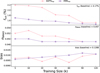 |
Fig. 4 Influence of training sample size on imputation performance. We show the photo-z metrics after imputation with the SAITS (pink) and KNN (purple) models for different training sample sizes. The nonimputed test set has a missing rate of 10%, and the corresponding metrics are shown in the upper-right corner of each panel. |
 |
Fig. 5 Influence of training sets with different missing rates on model performance. Training sets with missing rates of 10, 20, and 30% are used. Blue bars show baseline results from the nonimputed test set (with three bands removed), while pink and purple bars show results after imputation with the KNN and SAITS models, respectively. |
 |
Fig. 6 Spatial distribution of missing data for each photometric band in the input catalog. Gray points show all sources, while red points indicate sources with missing data in each band. A higher density of red points corresponds to a higher fraction of missing data. |
 |
Fig. 7 Magnitude distributions of the total source population (blue) and sources with missing data in the output catalog despite being present in the input catalog (pink).The dashed green line shows the magnitude limit of the corresponding CSST band. |
Evaluation metrics for photo-z estimations of the test set with three bands dropped after imputation with models trained on datasets with different missing rates.
5 Application on the missing data types of CSST
5.1 Missing data properties
Having established model performance under idealized MCAR conditions, we now turn to more complex and realistic missing data patterns found in simulated CSST catalogs. Such kind of data typically contains a mixture of all three missing types: MCAR, MAR, and MNAR.
First, the input simulated catalog contains predefined gaps. As illustrated by the spatial distribution in Figure 6, this missingness arises from two primary mechanisms. The first is the survey strategy, where edge regions of the footprint lack coverage, resulting in missing data that depends on sky coordinates; this is classified as MAR. The second mechanism involves detection limits, where the simulated observation depth aligns with the survey design. Sources fainter than the magnitude limits are intentionally marked as missing - a classic case of MNAR, as the missingness is inherently dependent on the brightness of the source. This is particularly notable in the NUV, u, and y bands, which have shallower depths. Overall, the predefined missing data in the input catalog is dominated by the MNAR mechanism.
Second, additional missingness is introduced in the final output catalog due to simulated observational image detection and pipeline processing. Figure 7 shows the magnitude distribution of sources that were present in the input simulation but were not detected in the output catalog, this missingness occurs for both faint and bright galaxies. Faint galaxies which fall below the signal-to-noise detection threshold are marginally detected, which again constitutes MNAR. For bright sources, however, the reasons for missingness are more complex, including image artifacts, source blending, or other stochastic processing failures. Since this type of missingness is independent of the source’s faintness, it is better described as a combination of MCAR and MAR. Based on an approximate estimate derived from the magnitude limits, MNAR-type missingness accounts for on the order of 30% of the additional missingness in the output catalog. However, after applying commonly sample selection criteria -retaining only galaxies with detections in more than three photometric bands and with S/N > 10 in the g or r band - this fraction is reduced to about 6%. Consequently, the additional missingness in the filtered dataset is dominated by MCAR and MAR components, with MNAR playing a relatively minor role.
 |
Fig. 8 Schematic illustration of the missing data processing in the input catalog based on the missing pattern of the output catalog. |
5.2 Data preparation
The dataset used here is no longer a complete subsample of the input catalog, but instead consists of all galaxies from the input catalog with high quality output photometry and detections in at least two bands. The final dataset contains 1 386 031 galaxies with an overall missing data fraction of 36%. This fraction rises to 44% when considering only the subset of galaxies with missing data. To create a realistic testbed for our imputation models, one that mirrors the complex missing data patterns of the final CSST survey while avoiding artifacts from the simulation pipeline, we devised a specific data preparation strategy. The core of this strategy is to map the missingness pattern from the output catalog onto the pristine input catalog. This approach allows us to work with the ground-truth photometry of the input simulation while testing the models against a realistic, multimechanism missing data pattern. The procedure is as follows:
Map missingness pattern: the missingness pattern from the output catalog is mapped onto the input catalog (Figure 8). This process generates two distinct flags for missing values. Values originally missing in the input catalog are marked as -99; these are primarily systematic MNAR cases resulting from magnitude limit cuts. Values present in the input catalog but missing in the output are marked as NAN; these represent the more stochastic MCAR/MAR cases arising from observational simulation and pipeline processing.
Partition dataset: the dataset is partitioned according to the logic illustrated in Figure 9. First, we divide the entire dataset into a complete subset (no missing values) and an incomplete subset (at least one band missing, the overall missing rate is 44%). The validation set is drawn exclusively from the complete subset, while the test set is drawn exclusively from the incomplete subset. The remaining data are combined to form a pool for constructing the training sets with different missing rates.
Training data sampling: constructed four distinct training sets from the training pool for our experiments: (a) a complete training set derived from the remaining complete data, and (b) three incomplete training sets with overall missing fractions of 10, 20, and 44% by mixing the remaining complete and incomplete dataset with different ratios.
 |
Fig. 9 Dataset partitioning scheme of the CSST mock data. The subsets and their missing rates are shown, with numbers in parentheses indicating the number of sources. |
 |
Fig. 10 Effect of training set missing rates on model performance for realistic CSST missing-pattern data. The missing rates of the training sets are set to 0, 10, 20, and 44%, respectively. Blue bars show the baseline results on nonimputed test set (44% missing rate), while pink and purple bars display results after KNN and SAITS imputation, respectively. |
5.3 Results analysis
In this section, we evaluate the performance of the imputation models on a fixed test set with an overall missing data fraction of 44%, consistent with the estimated missing rate from the CSST observational simulation. To investigate how the missing rate of the training dataset affects the model performance, we train both the KNN and SAITS models on four distinct training datasets described in Section 5.2.
The results, presented in Figure 10, reveal an crucial insight that differs from the trend observed in our idealized experiments in Section 4. In those experiments, where the datasets contain only MCAR-type missing values, lower missing rates consistently lead to higher photo-z accuracy (Figure 5). In contrast, under the more realistic setting considered here, where the data exhibit a mixture of MCAR, MAR, and MNAR missing patterns, training on incomplete data yields significantly better imputation performance than training on fully complete datasets. The optimal performance is achieved when the training set’s missing fraction matches that of the test set (44%). In this scenario, SAITS reduces the photo-z outlier fraction by nearly half, from a baseline of 55.83% for the nonimputed data down to 28.38%, and consistently outperforms KNN. These results demonstrate that, for real-world applications, training an imputation model on data that statistically mirrors the target dataset, in terms of both the quantity and the pattern of missingness, is crucial for achieving optimal performance.
To investigate the imputation performance on different missing data patterns, we first filtered the test set to include only galaxies with detections in more than three bands photometry and S/N > 10 in the g or r band, and classified the subset into three mutually exclusive groups based on their missing data flags described in Section 5.2:
MCAR/MAR group (Only NAN flag): galaxies where all missing bands were pipeline-induced.
MNAR group (Only -99 flag): galaxies where all missing bands were predefined by the magnitude limit.
Mix group: galaxies that contain both missing types. The results of the best-performing SAITS model, summarized in Table 5, are notable. For the MCAR/MAR group, the imputation is highly effective, reducing the outlier fraction by a factor of two compared to the baseline. Conversely, for the MNAR group, imputation is detrimental, slightly degrading the photo-z accuracy to a level worse than the nonimputed data. Because a large fraction of missingness is driven by the survey magnitude limit, the overall outlier fraction decreases by only 5.6%.
This finding suggests a clear optimal strategy: selectively impute only the data known to be MCAR or MAR. We tested this hybrid strategy by imputing only the NAN-flagged values, while leaving the -99 values missing. As shown in Figure 11, this method yields the best overall performance, reducing the outlier fraction for these sources from 10.01% (with full imputation) to a superior 8.7%. This improvement arises because MNAR values, which are often driven by magnitude limits, tend to be imputed with artificially brighter fluxes, leading to systematically underestimated redshifts. This effect is visible at the high-redshift end of the middle panel in Figure 11, where missing measurements are more likely driven by the depth of the survey rather than random absence. These results demonstrate that although imputation is effective for MCAR/MAR missingness, it is preferable to avoid imputing values that are missing due to physical limits (MNAR), where the absence of information is itself informative for photo-z estimation.
For further investigation, we group galaxies by the number of missing bands and compute photo-z metrics for each subset separately. The results, presented in Table 6, show that galaxies with three missing bands exhibit substantially degraded photo-z performance in both the nonimputed and imputed cases. Therefore, for statistical analysis requiring high photo-z accuracy, it is conservative to restrict the sample to galaxies with fewer than three missing bands.
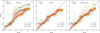 |
Fig. 11 Photo-z versus true values for test set galaxies with detections in more than three photometric bands and g or r band S/N > 10. The left panel shows results for the nonimputed test set. The middle panel shows results after SAITS imputation. The right panel shows results where “NAN” and “Mix” missing types are imputed with SAITS, while values flagged as “-99” are not imputed. |
Photo-z metrics for sources with different missing types.
6 Conclusions
This study presents a systematic evaluation of data imputation methods to improve photo-z estimation accuracy. Our investigation began by assessing a suite of ML and DL models to identify the top performers. We then subjected these leading models, KNN and SAITS, to comprehensive robustness tests, varying both the training sample size and the missing data rate. Finally, we evaluated their performance on a realistic testbed designed to represent the complex, mixed-mechanism missing data pattern of the CSST survey, providing a practical validation under real observational conditions.
Under idealized MCAR conditions with a complete training set, the deterministic KNN model provides the best overall imputation performance, closely followed by the attention-based SAITS model. Both models are remarkably data-efficient, maintaining high accuracy even with training datasets as small as 5000 samples. This specific finding reflects a broader trend among the different architectural foundations tested: among ML category, distance-based models such as KNN outperformed tree-based models, while in DL approaches, transformer-based models such as SAITS were superior.
The robustness of the models to incomplete training data differs starkly. KNN’s performance degrades sharply as the missing fraction of the training set increases. In contrast, SAITS demonstrates exceptional robustness, maintaining high performance even when trained on highly incomplete data.
When tested on the realistic, mixed-mechanism CSST missing data pattern, the performance ranking differs: SAITS consistently outperforms KNN, optimal results are achieved when the missing data pattern of the training set statistically mirrors that of the test set. This highlights a crucial principle for any supervised learning approach: maintaining domain consistency between training and testing samples, where the distributions of both features and targets are aligned, is critical for regression-based tasks such as imputation.
Although creating domain-consistent datasets is relatively straightforward for an imputation task, it is considerably more challenging for many other regression problems in astronomy. Practical observational datasets are often highly imbalanced and subject to complex selection biases, which must be carefully assessed when deploying supervised learning techniques. Consequently, a model trained and validated on a domain-consistent dataset is likely to experience performance degradation when applied to real-world scenarios where a “domain shift” exists. Researchers must be cautious about this issue and consider strategies such as domain adaptation to address its impact. Otherwise, accuracy assessments derived from idealized test datasets may not serve as reliable indicators of real-world performance.
For the mixed types of missing data common in practical observations, we find that while general imputation models such as SAITS are highly effective for MCAR and MAR data, they are detrimental for MNAR data. In multiband photometry, MNAR data primarily arise from magnitude-limited observations, meaning the missingness itself contains physical information. Statistical models such as SAITS are designed to minimize the reconstruction error based on the available data distribution, which is often biased toward brighter sources in supervised training sets.
A straightforward and effective strategy is therefore to impute only MAR and MCAR data, while leaving MNAR values untouched. Implementing this requires forced photometry that can distinguish between stochastic missingness (MCAR/MAR) and nondetection (MNAR). We also attempted to teach the model the MNAR pattern by training on deep-field data, but this strategy was ineffective, demonstrating that the MNAR pattern is not a purely statistical phenomenon that can be learned by proxy.
This inherent characteristic of astronomical data is difficult to incorporate as a constraint into general-purpose imputation models. We therefore recommend the development of specialized architectures capable of disentangling these distinct missingness mechanisms. Such models should treat stochastic gaps (MCAR/MAR) through traditional reconstruction while incorporating magnitude limits as informative priors for MNAR, thereby preserving the physical integrity of the completed catalog.
Photo-z metrics for test set galaxies missing 1-3 bands with detections in more than three photometric bands and g- or r-band S/N > 10.
Acknowledgements
This work is supported by the China Manned Space Project with Grant NO. CMS-CSST-2021-A07, No. CMS-CSST-2021-A01, and NO. CMS-CSST-2025-A05, Z.C. and L.P.F. acknowledge support from NSFC grant No. 12541302, No. 12141302, and the Innovation Program of Shanghai Municipal Education Commission (Grant No. 2025GDZKZD04).
References
- Abdalla, F. B., Banerji, M., Lahav, O., & Rashkov, V. 2011, MNRAS, 417, 1891 [NASA ADS] [CrossRef] [Google Scholar]
- Agarwal, S. 2013, in 2013 International Conference on Machine Intelligence and Research Advancement, 203 [Google Scholar]
- Agarwal, N., Dalal, S. R., & Misra, V. 2025, arXiv e-prints [arXiv:2512.22471] [Google Scholar]
- Akiba, T., Sano, S., Yanase, T., Ohta, T., & Koyama, M. 2019, in Proceedings of the 25th ACM SIGKDD International Conference on Knowledge Discovery and Data Mining [Google Scholar]
- Ban, Z., Li, X.-B., Yang, X., et al. 2026, Res. Astron. Astrophys., 26, 024002 [Google Scholar]
- Bolzonella, M., Miralles, J. M., & Pelló, R. 2000, A&A, 363, 476 [NASA ADS] [Google Scholar]
- Brammer, G. B., van Dokkum, P. G., & Coppi, P. 2008, ApJ, 686, 1503 [Google Scholar]
- Breiman, L. 2001, J. Clinical Microbiol., 2, 199 [Google Scholar]
- Cao, W., Wang, D., Li, J., et al. 2018a, in Advances in Neural Information Processing Systems (New York: Curran Associates, Inc.), 31 [Google Scholar]
- Cao, Y., Gong, Y., Meng, X.-M., et al. 2018b, MNRAS, 480, 2178 [Google Scholar]
- Cao, Y., Gong, Y., Zheng, Z.-Y., & Xu, C. 2022, Res. Astron. Astrophys., 22, 025019 [CrossRef] [Google Scholar]
- Carrasco Kind, M., & Brunner, R. J. 2013, MNRAS, 432, 1483 [Google Scholar]
- Chartab, N., Mobasher, B., Cooray, A. R., et al. 2023, ApJ, 942, 91 [Google Scholar]
- Cole, S., Percival, W. J., Peacock, J. A., et al. 2005, MNRAS, 362, 505 [Google Scholar]
- Conroy, C., Gunn, J. E., & White, M. 2009, ApJ, 699, 486 [Google Scholar]
- Conselice, C. J. 2014, ARA&A, 52, 291 [CrossRef] [Google Scholar]
- Cover, T., & Hart, P. 1967, IEEE Trans. Inform. Theory, 13, 21 [CrossRef] [Google Scholar]
- CSST Collaboration (Gong, Y., et al.) 2026, Sci. China Phys. Mech. Astron., 69, 239501 [Google Scholar]
- Demirtas, H. 2018, J. Stat. Softw. Book Rev., 85, 1 [Google Scholar]
- Desprez, G., Paltani, S., Coupon, J., et al. 2020, A&A, 644, A31 [NASA ADS] [CrossRef] [EDP Sciences] [Google Scholar]
- Dey, A., Schlegel, D. J., Lang, D., et al. 2019, AJ, 157, 168 [Google Scholar]
- Du, W., Côté, D., & Liu, Y. 2023a, Expert Syst. Appl., 219, 119619 [Google Scholar]
- Du, W., Yang, Y., Qian, L., Wang, J., & Wen, Q. 2023b, arXiv e-prints [arXiv:2305.18811] [Google Scholar]
- Euclid Collaboration (Tucci, M., et al.) 2025, A&A, accepted [arXiv:2503.15306] [Google Scholar]
- Feldmann, R., Carollo, C. M., Porciani, C., et al. 2006, MNRAS, 372, 565 [NASA ADS] [CrossRef] [Google Scholar]
- Fortuin, V., Baranchuk, D., Raetsch, G., & Mandt, S. 2020, in Proceedings of Machine Learning Research, 108, Proceedings of the Twenty Third International Conference on Artificial Intelligence and Statistics, ed. S. Chiappa & R. Calandra (PMLR), 1651 [Google Scholar]
- Fotopoulou, S., & Paltani, S. 2018, A&A, 619, A14 [NASA ADS] [CrossRef] [EDP Sciences] [Google Scholar]
- Gong, Y., Liu, X., Cao, Y., et al. 2019, ApJ, 883, 203 [NASA ADS] [CrossRef] [Google Scholar]
- Graham, J. W. 2009, Ann. Rev. Psychol., 60, 549 [Google Scholar]
- Han, J., Li, M., Jiang, W., et al. 2025, Sci. China Phys. Mech. Astron., 68, 109511 [Google Scholar]
- Ilbert, O., Arnouts, S., McCracken, H. J., et al. 2006, A&A, 457, 841 [NASA ADS] [CrossRef] [EDP Sciences] [Google Scholar]
- Ivezić, Z., Kahn, S. M., Tyson, J. A., et al. 2019, ApJ, 873, 111 [NASA ADS] [CrossRef] [Google Scholar]
- Keerin, P., & Boongoen, T. 2022, Inform. Process. Management, 59, 102881 [Google Scholar]
- Koo, D. C. 1985, AJ, 90, 418 [NASA ADS] [CrossRef] [Google Scholar]
- La Torre, V., Sajina, A., Goulding, A. D., et al. 2024, AJ, 167, 261 [Google Scholar]
- Laureijs, R., Amiaux, J., Arduini, S., et al. 2011, arXiv e-prints [arXiv:1110.3193] [Google Scholar]
- Little, R., & Rubin, D. 2019, Statistical Analysis with Missing Data, 3rd edn. (Hoboken: Wiley) [Google Scholar]
- Liu, D. Z., Meng, X. M., Er, X. Z., et al. 2023, A&A, 669, A128 [NASA ADS] [CrossRef] [EDP Sciences] [Google Scholar]
- Liu, Y., Hu, T., Zhang, H., et al. 2024, in The Twelfth International Conference on Learning Representations [Google Scholar]
- Loh, E. D., & Spillar, E. J. 1986, ApJ, 303, 154 [NASA ADS] [CrossRef] [Google Scholar]
- LSST Science Collaboration (Abell, P. A., et al.) 2009, arXiv e-prints [arXiv:0912.0201] [Google Scholar]
- Luken, K. J., Padhy, R., & Wang, X. R. 2021, in Machine Learning for Physical Sciences workshop at NeurIPS 2021, 1 [Google Scholar]
- Luo, Z., Tang, Z., Chen, Z., et al. 2024, MNRAS, 531, 3539 [Google Scholar]
- Ma, Z., Tian, H., Liu, Z., & Zhang, Z. 2020, Appl. Soft Comput., 90, 106175 [Google Scholar]
- Miao, X., Wu, Y., Wang, J., et al. 2021, Proc. AAAI Conf. Artif. Intell., 35, 8983 [Google Scholar]
- Mo, H., van den Bosch, F. C., & White, S. 2010, Galaxy Formation and Evolution (Cambridge, UK: Cambridge University Press) [Google Scholar]
- Pedregosa, F., Varoquaux, G., Gramfort, A., et al. 2011, J. Mach. Learn. Res., 12, 2825 [Google Scholar]
- Percival, W. J., Nichol, R. C., Eisenstein, D. J., et al. 2007, ApJ, 657, 645 [NASA ADS] [CrossRef] [Google Scholar]
- Prokhorenkova, L., Gusev, G., Vorobev, A., Dorogush, A. V., & Gulin, A. 2018, in Proceedings of the 32nd International Conference on Neural Information Processing Systems, NIPS’18 (Red Hook, NY, USA: Curran Associates Inc.), 6639 [Google Scholar]
- Salvato, M., Ilbert, O., & Hoyle, B. 2019, Nat. Astron., 3, 212 [NASA ADS] [CrossRef] [Google Scholar]
- Schindler, J.-T., Fan, X., McGreer, I. D., et al. 2017, ApJ, 851, 13 [NASA ADS] [CrossRef] [Google Scholar]
- Tasca, L. A. M., Kneib, J. P., Iovino, A., et al. 2009, A&A, 503, 379 [NASA ADS] [CrossRef] [EDP Sciences] [Google Scholar]
- Van Buuren, S. 2000, Multivariate imputation by chained equations: MICE V1. 0 user’s manual (Leiden: TNO) [Google Scholar]
- Vaswani, A., Shazeer, N., Parmar, N., et al. 2017, in Advances in Neural Information Processing Systems, eds. I. Guyon, U. V. Luxburg, S. Bengio, H. Wallach, R. Fergus, S. Vishwanathan, & R. Garnett (New York: Curran Associates, Inc.), 30 [Google Scholar]
- Venkatraman, R., & Khaitan, S. K. 2015, in 2015 IEEE Power & Energy Society General Meeting, 996 [Google Scholar]
- Veronika Dorogush, A., Ershov, V., & Gulin, A. 2018, arXiv e-prints [arXiv:1810.11363] [Google Scholar]
- Wang, A., Chen, Y., An, N., et al. 2019, IEEE/ACM Trans. Comput. Biol. Bioinform., 16, 980 [Google Scholar]
- Wei, C.-L., Li, G.-L., Fang, Y.-D., et al. 2026a, Res. Astron. Astrophys., 26, 024001 [Google Scholar]
- Wei, C.-L., Luo, Y., Tian, H., et al. 2026b, Res. Astron. Astrophys., 26, 024004 [Google Scholar]
- Xian, J.-T., Lin, L., Fang, Y.-D., et al. 2026, Res. Astron. Astrophys., 26, 024005 [Google Scholar]
- Yoon, J., Jordon, J., & Schaar, M. 2018, in International conference on machine learning, PMLR, 5689 [Google Scholar]
- Yoon, J., Zame, W. R., & van der Schaar, M. 2019, IEEE Trans. Biomed. Eng., 66, 1477 [Google Scholar]
- Zhan, H. 2011, Scientia Sinica Physica, Mechanica & Astronomica, 41, 1441 [Google Scholar]
- Zhan, H. 2021, Chinese Sci. Bull., 66, 1290 [CrossRef] [Google Scholar]
Appendix A Imputation performance validation of the model in the output catalog
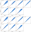 |
Fig. A.1 Same as Figure 2, but for the output catalog. Panel a: Predicted versus true magnitudes (KNN). Panel b: Same as (a) but for the SAITS model. |
All Tables
Number of model parameters and training time per epoch for different numbers of missing bands.
Evaluation metrics for photo-z estimations of the test set with three bands dropped after imputation with models trained on datasets with different missing rates.
Photo-z metrics for test set galaxies missing 1-3 bands with detections in more than three photometric bands and g- or r-band S/N > 10.
All Figures
|
Fig. 1 Flux-error relations across bands. Input flux versus predicted flux errors (pink) and output catalog values (blue). |
| In the text | |
|
Fig. 2 Predicted versus true magnitudes for the test set with three missing photometric bands using the imputation models. Panel a: predicted versus true magnitudes (KNN). Panel b: same as (a) but for the SAITS model. We show the predicted values as a function of the true values. The dashed green line marks mag predict = mag true, and the red line shows the linear fit. |
| In the text | |
|
Fig. 3 Photo-z quality metrics for the KNN and SAITS models for test sets with different missing data rates. Blue bars show the SED fitting on nonimputed data, and pink and purple bars show results after KNN and SAITS imputation, respectively. |
| In the text | |
|
Fig. 4 Influence of training sample size on imputation performance. We show the photo-z metrics after imputation with the SAITS (pink) and KNN (purple) models for different training sample sizes. The nonimputed test set has a missing rate of 10%, and the corresponding metrics are shown in the upper-right corner of each panel. |
| In the text | |
|
Fig. 5 Influence of training sets with different missing rates on model performance. Training sets with missing rates of 10, 20, and 30% are used. Blue bars show baseline results from the nonimputed test set (with three bands removed), while pink and purple bars show results after imputation with the KNN and SAITS models, respectively. |
| In the text | |
|
Fig. 6 Spatial distribution of missing data for each photometric band in the input catalog. Gray points show all sources, while red points indicate sources with missing data in each band. A higher density of red points corresponds to a higher fraction of missing data. |
| In the text | |
|
Fig. 7 Magnitude distributions of the total source population (blue) and sources with missing data in the output catalog despite being present in the input catalog (pink).The dashed green line shows the magnitude limit of the corresponding CSST band. |
| In the text | |
|
Fig. 8 Schematic illustration of the missing data processing in the input catalog based on the missing pattern of the output catalog. |
| In the text | |
|
Fig. 9 Dataset partitioning scheme of the CSST mock data. The subsets and their missing rates are shown, with numbers in parentheses indicating the number of sources. |
| In the text | |
|
Fig. 10 Effect of training set missing rates on model performance for realistic CSST missing-pattern data. The missing rates of the training sets are set to 0, 10, 20, and 44%, respectively. Blue bars show the baseline results on nonimputed test set (44% missing rate), while pink and purple bars display results after KNN and SAITS imputation, respectively. |
| In the text | |
|
Fig. 11 Photo-z versus true values for test set galaxies with detections in more than three photometric bands and g or r band S/N > 10. The left panel shows results for the nonimputed test set. The middle panel shows results after SAITS imputation. The right panel shows results where “NAN” and “Mix” missing types are imputed with SAITS, while values flagged as “-99” are not imputed. |
| In the text | |
|
Fig. A.1 Same as Figure 2, but for the output catalog. Panel a: Predicted versus true magnitudes (KNN). Panel b: Same as (a) but for the SAITS model. |
| In the text | |
Current usage metrics show cumulative count of Article Views (full-text article views including HTML views, PDF and ePub downloads, according to the available data) and Abstracts Views on Vision4Press platform.
Data correspond to usage on the plateform after 2015. The current usage metrics is available 48-96 hours after online publication and is updated daily on week days.
Initial download of the metrics may take a while.