| Issue |
A&A
Volume 709, May 2026
|
|
|---|---|---|
| Article Number | A126 | |
| Number of page(s) | 17 | |
| Section | Stellar structure and evolution | |
| DOI | https://doi.org/10.1051/0004-6361/202659115 | |
| Published online | 12 May 2026 | |
Cyclic light variations and accretion disk evolution in the Large Magellanic Cloud eclipsing binary OGLE-LMC-DPV-062
1
Universidad de Concepción, Departamento de Astronomía, Casilla 160-C, Concepción, Chile
2
Astronomical Observatory, Volgina 7, 11060 Belgrade, Serbia
3
Issac Newton Institute of Chile, Yugoslavia Branch, 11060 Belgrade, Serbia
4
Instituto de Física y Astronomía, Universidad de Valparaíso, Gran Bretaña 1111, Playa Ancha, Valparaíso, Chile
5
Dipartimento di Fisica, Sapienza Università di Roma, Piazzale Aldo Moro 5, 00185, Rome, Italy
6
Astronomical Observatory, University of Warsaw, Al. Ujazdowskie 4, 00-478 Warszawa, Poland
★ Corresponding author: This email address is being protected from spambots. You need JavaScript enabled to view it.
Received:
24
January
2026
Accepted:
16
March
2026
Abstract
Context. Many intermediate-mass close binaries exhibit photometric cycles longer than their orbital periods, likely linked to variations in their accretion disks. Previous studies suggest that analyzing historical light curves provides key insights into disk evolution and may help track changes in mass transfer rates in such systems.
Aims. Our research explores short- and long-term fluctuations in the eclipsing system OGLE-LMC-DPV-062, focusing on the variability of its long cycle. We aim to clarify the role of the accretion disk in these modulations, especially those spanning hundreds of days, and to determine the system’s evolutionary status to better understand its stellar components.
Methods. We analyzed 32.3 years of photometric time series from the Optical Gravitational Lensing Experiment (OGLE) in the I and V bands, and from the MAssive Compact Halo Objects (MACHO) project in BM and RM bands. Using data from multiple epochs, we modeled the accretion disk across 20 equally spaced phases of the long cycle. To solve the inverse problem, we implemented an optimized simplex algorithm to determine the best parameters for the stars, their orbit, and the disk. The Modules for Experiments in Stellar Astrophysics (MESA) code was employed to assess the system’s evolutionary stage and predict its past and future development.
Results. We find an orbital period of 6.d904858(15) and a long cycle of 229.d7. Our orbital solutions reproduce the light curves, but the quasi-conservative mass transfer scenario yields rates that are too high for the orbital period stability. We find a consistency with the observed orbital-to-long-period ratio under the magnetic dynamo hypothesis. The normalized mass transfer rate follows the long cycle, reaching a maximum when brightness is minimum. At that phase, the disk’s inner edge thickens, obscuring more of the gainer star. Disk variability mainly occurs in its vertical extension, with a standard deviation of 69% the mean value at the inner border, with minor changes in the outer radius and temperature of 7% and 5%, respectively.
Key words: accretion / accretion disks / binaries close / binaries: eclipsing / binaries: general / stars: evolution
© The Authors 2026
 Open Access article, published by EDP Sciences, under the terms of the Creative Commons Attribution License (https://creativecommons.org/licenses/by/4.0), which permits unrestricted use, distribution, and reproduction in any medium, provided the original work is properly cited.
This article is published in open access under the Subscribe to Open model. This email address is being protected from spambots. You need JavaScript enabled to view it. to support open access publication.
1. Introduction
Interacting binary stars serve as intricate natural laboratories for exploring a wide array of astrophysical processes. These processes include accretion disk physics, stellar winds, gas dynamics in mass transfer, angular momentum loss and redistribution, stellar rotation, and tidal interactions. A substantial fraction of stars are thought to belong to multiple systems, with close gravitational interactions between stellar components being a common occurrence across the Universe. Some of the most energetic events observed to date – such as black hole or neutron star mergers – are interpreted as the end products of binary evolution involving previous episodes of mass exchange and angular momentum loss. The study of interacting close binaries is rooted in the foundational framework established by Paczyński (1971), who described the key evolutionary processes governing mass exchange in such systems. The geometrical constraints imposed by Roche-lobe overflow are commonly quantified using the widely adopted approximation of Eggleton (1983), while the interpretation of eclipsing-binary light curves has long relied on the formalism introduced by Wilson & Devinney (1971). Together, these works provide the basic theoretical and methodological context for analyzing semidetached interacting binaries. A comprehensive review of binary star evolution can be found in Eggleton (2021).
Among the diverse family of interacting binary stars, a particularly intriguing subclass – known as double periodic variables (DPVs) – exhibits two distinct photometric periodicities: an orbital period and a longer, quasi-cyclic variability whose origin remains unresolved (Mennickent et al. 2003; Mennickent 2017; Garcés et al. 2025). These long cycles typically exceed the orbital period by a factor of 20–40, with amplitudes around 0.1–0.2 mag in the I band. DPVs are semidetached binaries comprising a B-type main-sequence star (the gainer) surrounded by an optically thick accretion disk, which is sustained by mass transfer from a less massive, Roche-lobe-filling late-type giant star (the donor) with a typical mass of around one solar mass. The B-type component has been “rejuvenated” by the accretion of hydrogen-rich material from its companion (Rosales et al. 2024).
More than 200 DPVs have been identified in the Milky Way and the Magellanic Clouds (Mennickent et al. 2003, 2016; Poleski et al. 2010; Pawlak et al. 2013; Rojas et al. 2021; Głowacki et al. 2024). Detailed studies show that these systems tend to exhibit higher luminosities and effective temperatures than typical Algol-type binaries, likely reflecting different evolutionary states or mass transfer histories (Mennickent et al. 2016). Notable Galactic examples of DPVs include RX Cas (Gaposchkin 1944), AU Mon (Lorenzi 1980), β Lyrae (Guinan 1989), V 360 Lac (Hill et al. 1997), and CX Dra (Koubsky et al. 1998).
The nature of the long photometric cycle remains an open question. One of the most promising hypotheses invokes a magnetic dynamo operating within the convective envelope of the donor star (Schleicher & Mennickent 2017). This mechanism could modulate the star’s quadrupole moment, producing periodic variations in the mass transfer rate and, consequently, in the structure and brightness of the accretion disk. In this scenario, the observed photometric changes during the long cycle arise from alterations in the disk’s radial and vertical dimensions. While this model is supported by correlations between the long-cycle phase and disk properties in several systems (e.g., Garcés et al. 2018; Mennickent et al. 2025; Mennickent & Djurašević 2025), direct evidence of such a stellar dynamo is still lacking. Further observational and theoretical studies are required to confirm its existence and fully characterize the long-term variability of DPVs.
In this paper we present the first combined photometric analysis of OGLE-LMC-DPV-062, covering 30 years of data, to study the disk variability along the long cycle and its evolutionary implications. This binary is also known as OGLE-LMC-ECL-12848, OGLE J051941.10−693117.1, and MACHO 78.6343.81 (Graczyk et al. 2011; Pawlak et al. 2016). The astrometric and photometric properties of the system include α2000 = 05:19:41.00, δ2000 = −69:31:17.0, B = 15.960 mag, V = 15.925 mag, R = 15.863 mag and I= 15.823 mag and V = 18.001 mag1. The Gaia DR3 catalog provides mean magnitudes of G = 15.9879 ± 0.0095 mag, BP = 15.9160 ± 0.0238, RP = 15.7616 ± 0.0228 mag, and BP − RP = 0.1544 ± 0.0329 mag2. The same source provides an extinction of AG = 0.6391 (0.6317,0.6468) mag. The target was classified as a DPV with an orbital period of 6 9044 ± 0
 0010 and a long period of 226 ± 13 days (Mennickent et al. 2003). Later, the reported orbital period was improved to 6
 904830 ± 0
 000015 and the long period to 229
 080 ± 0
 062 (Poleski et al. 2010).
OGLE-LMC-DPV-062 was selected for this study because of its relatively large photometric variability produced by the combined orbital and long-term cycles. In addition, its long-term modulation is traced across more than three decades of photometry, enabling a quantitative test of the hypothesis that changes in the disk structure produce the long-term cycle.
2. Data and methodology
2.1. Photometric data
The photometric time series analyzed in this study consists of 8942 I-band data points and 495 V-band data points obtained by the Optical Gravitational Lensing Experiment (OGLE, Udalski et al. 2015). The I-band light curve shows the typical variability of an eclipsing binary, plus a remarkable long-term variability (Fig. 1). In addition, we study 1606 BM and 1557 RM data points obtained by the MAssive Compact Halo Objects (MACHO) project3. The two MACHO passbands are nonstandard. The blue band covers 437–590 nm with an effective wavelength of about 520 nm, and the red band covers 590–780 nm with an effective wavelength of about 690 nm. A detailed description of the MACHO photometric system is given by Alcock et al. (1997). The whole dataset, summarized in Table 1, spans a time interval of 32.3 yr.
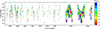 |
Fig. 1. Section of the OGLE I-band light curve of OGLE-LMC-DPV-062. Colors indicate different orbital phases. |
Photometric observations.
2.2. Time series analysis
We used phase dispersion minimization (PDM, Stellingwerf 1978) and the generalized Lomb Scargle software (GLS, Zechmeister & Kürster 2009) to detect periodicities in the light curve. Long-term tendencies were studied with the weighted wavelet Z transform WWZ as defined by Foster (1996). Each I and RM light curve was shifted to a common mean magnitude before applying this transform. The WWZ works in a similar way to the Lomb-Scargle periodogram providing information about the periods of the signal and the time associated with those periods. It is very suitable for the analysis of nonstationary signals and has advantages for the analysis of local time-frequency characteristics. In order to search for the long-term cycle length, we removed the contribution of the orbital cycle from the observed light curve by fitting a Fourier series to the photometry. This fit was performed using the orbital phase, calculated from the system’s ephemeris, and the observed magnitude as a function of phase. The Fourier function included 16 harmonics, which allowed for an accurate reproduction of the orbital light curve morphology. The fit was carried out using the curve-fit function from scipy.optimize, optimizing the coefficients of the Fourier series. Once the optimal parameters were obtained, the fit model was calculated, and the observed magnitudes were subtracted, yielding the residuals that entered into the WWZ algorithm.
2.3. The light curve model
The inverse problem was solved using a sophisticated simplex algorithm (Dennis & Torczon 1991), allowing us to fit the observed light curve by optimizing the parameters of the star−orbit−disk configuration. The foundations of this method and the procedure for generating synthetic light curves are extensively described in the literature (Djurašević 1992, 1996), with further enhancements reported by Djurašević et al. (2008). This modeling approach has been successfully applied in the analysis of numerous interacting binaries (e.g., Mennickent & Djurašević 2013; Rosales 2018; Mennickent et al. 2020b).
The total flux from the system was modeled as the sum of the stellar contributions plus the emission from an optically thick accretion disk surrounding the more luminous component, with projection effects modulated by the orbital inclination. The disk’s emission was calculated using local Planck functions at characteristic temperatures, neglecting detailed radiative transfer. Nonetheless, the model accounts for reflection effects, limb darkening, and gravity darkening of the stars.
The accretion disk is described by its radius, Rd, its vertical semi-thicknesses at the center and outer edge (dc and de, respectively), and a radially varying temperature profile (e.g., Brož et al. 2021):
 (1)
(1)
where Td denotes the temperature at the disk’s outer rim (r = Rd) and aT is the radial temperature gradient exponent, constrained to aT ≤ 0.75. When aT = 0.75, the profile corresponds to a steady-state configuration. This temperature law reflects a hotter inner disk region that gradually cools toward the outer edge.
The model also includes two localized active regions at the disk rim: the hot spot, placed near the expected impact site of the gas stream from the inner Lagrangian point, and the bright spot, located at a different azimuth. Both regions are assumed to be hotter and vertically more extended than the surrounding disk, in agreement with Doppler tomography and hydrodynamical studies of interacting binaries (e.g., Albright & Richards 1996; Bisikalo et al. 2000; Atwood-Stone et al. 2012). Similar structures have also been inferred in the DPV β Lyrae from light-curve modeling, interferometry, and polarimetry (Mennickent & Djurašević 2013; Lomax et al. 2012; Mourard et al. 2018). While the hot spot is naturally associated with the interaction between the stream and the disk, the bright spot may arise from gas that has crossed the shock discontinuity region between the stream and the disk (the so-called hot line) and then flows along the outer disk rim with enhanced vertical motion. Hydrodynamical calculations show that this process can produce vertical oscillations and secondary thickened regions at other azimuths, providing a plausible physical origin for the bright spot (Kaigorodov et al. 2017).
Each spot is characterized by a relative temperature, Ahs ≡ Ths/Td for the hot spot and Abs ≡ Tbs/Td for the bright spot, their angular extents (θhs and θbs), and azimuthal positions with respect to the line of centers in the direction of orbital motion (λhs and λbs). The parameter θrad denotes the angle between the local disk surface normal and the direction of peak radiation from the hot spot.
We acknowledge that the model described above is a simplified representation of the disk rather than a comprehensive physical simulation. Nevertheless, as we shall demonstrate later, it enables the extraction of certain physical parameters and the description of the system photometric variability in terms of variations in disk parameters.
For gravity darkening, the coefficients are set to β1 = 0.25 and β2 = 0.08, corresponding to radiative and convective envelopes, respectively, while the albedos are A1 = 1.0 and A2 = 0.5, in line with von Zeipel’s law for radiative flux redistribution (von Zeipel 1924). Limb darkening was modeled using the four-coefficient nonlinear law of Claret (2000), with the passband-specific coefficients recalculated at each iteration by bilinear interpolation in Teff and log g from tabulated values for the relevant photometric bands; the same prescription was also applied to the disk (Djurašević et al. 2010).
In addition, we calculated the relative mass transfer rate, Ṁ, using the approximation given by Mennickent & Djurašević (2021)
![Mathematical equation: $$ \begin{aligned} \frac{\dot{M}_{2,f}}{\dot{M}_{2,i}}= \frac{ {{R}^2_{\rm disk,f}} [A_{\rm hs,f}T_{\rm disk,f}]^{4} d_{\rm e,f} \theta _{\rm hs,f} }{{{R}^2_{\rm disk,i}} [A_{\rm hs,i}T_{\rm disk,i}]^{4} d_{\rm e,i} \theta _{\rm hs,i}}. \end{aligned} $$](/articles/aa/full_html/2026/05/aa59115-26/aa59115-26-eq11.gif) (2)
(2)
This formula assumes a hot spot along the disk border whose luminosity is due to the release of gravitational energy when the gas stream coming from the inner Lagrangian point impacts its surface. This approximation enables us to calculate the relative mass transfer rates at various times, denoted by epochs i and f, within a specific system.
2.4. The evolutionary code
For the calculation of the evolution of the possible DPV062 progenitor binary systems, the MESA (Modules for Experiments in Stellar Astrophysics) code (Paxton et al. 2011, 2013, 2015; Paxton et al. 2018) was used, in revision 10398. This code calculates the detailed evolution of both stars. The stellar wind mass loss rate of each star is calculated according to Vink et al. (2001) for stars with a surface abundance of hydrogen above 0.4 and Nugis & Lamers (2000) for a hydrogen abundance below 0.4. The matter lost due to the stellar wind has the specific orbital angular momentum of its star. The mass transfer rate is calculated according to Ritter (1988). The composition of accreted material is identical to the donor’s current surface composition. The metallicity is set to the Large Magellanic Cloud (LMC) value of 0.006 (Eggenberger et al. 2021).
3. Results
3.1. Period analysis
Using the I band photometry and the PDM algorithm, we found the following ephemeris for the occultation of the cooler star:
 (3)
(3)
This finding was confirmed applying the GLS and it is consistent with the previous value given by Poleski et al. (2010). The analysis of the minima of the light curve confirmed that, for all practical purposes, the orbital period is constant.
We find that the WWZ transform for the I-band and RM time series suggests a rather stable long-term cycle length of around 230 days (Fig. 2). We determined the following ephemeris for the maximum of the long cycle:
 (4)
(4)
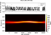 |
Fig. 2. WWZ transform showing a strong signal around 230 days. The orbital period was removed before the analysis. |
We note that this long period is longer than that reported by (Poleski et al. 2010), which may be attributable to the longer time series analyzed in the present study along with possible changes on a long-term variability timescale. We find that the shape of the orbital light curve changes according to the long-term cycle phase (Fig. 3). The overall system brightness follows the long-term cycle and the secondary minimum shifts around long-cycle phase 0.5. Changes are observed in the overall shape of the orbital light curve at different long-term cycle phases. The long-term cycle is revealed in slices of data taken at quadrature and primary eclipse (Fig. 4). While at quadrature the light curve shows a smooth oscillatory pattern, the data at main eclipse show a much larger scatter.
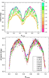 |
Fig. 3. Orbital light curve colored with the long-term cycle phase of the data. Magnitudes subtracting the minimum magnitude of the respective dataset are shown in the graph below. |
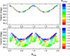 |
Fig. 4. I-band magnitudes taken at orbital phases [0.2–0.3; up] and [0.9–1.1; down] phased with the long-term cycle phase. |
3.2. MACHO colors and extinction
The MACHO light curve follows the behavior shown by the OGLE light curves but with a higher scatter (Fig. B.1). The photometry reveals that, except for eclipses, the main color trends are observed during the long cycle, not during the orbital cycle, and that these variations are of a rather small amplitude (Fig. B.2). The data also show that, in general, the system is redder when brighter, i.e., usually near the maximum of the long cycle. In addition, a color loop is observed. The rising branch shows bluer colors compared to the declining branch (Fig. 5), something also reported in the DPV OGLE05155332-6925581 (Mennickent et al. 2008).
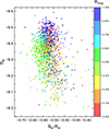 |
Fig. 5. MACHO BM − RM color versus orbital and long-term cycle phases. |
For the coordinates of OGLE-LMC-DPV-062, we obtained E(V − I) = 0.073 ± 0.100 following extinction maps in the LMC (Skowron et al. 2021). The extinction, AI, can generally be estimated as AI = 1.5 × E(V − I) (Iwanek et al. 2021). In our case, this is AI = 1.5 × 0.073 = 0.11 ± 0.15. Using AV = (2.5 ± 0.2) × E(V − I) (Iwanek et al. 2021), we get AV = 0.183 ± 0.015. We did not found extinction transformation coefficients for the MACHO R or B bands. Due to the complex nature and uncertainties involved in the MACHO photometry and the atypical bandpass filters (Alcock et al. 1999), we considered MACHO photometry only for the light curve models and eclipse timings.
3.3. The stellar parameters
The absence of spectroscopic data limits the accuracy of our knowledge of the stellar parameters; however, we can still obtain preliminary estimates, bearing in mind that spectroscopic studies are required to confirm them. Nevertheless, the general trends and patterns derived from the analysis of the long cycle are expected to remain robust against small variations in the adopted stellar parameters.
If the main eclipse is total, then the color observed at this epoch corresponds to the donor. As our system shows partial eclipses, the gainer (and eventually the disk) also contributes to the flux at minimum. This means that only an upper limit for the donor effective temperature can be derived from the system color at main eclipse. After a careful inspection of the I − V band light curves during main eclipse (between Φo = 0.95 and 1.05) around different long-term phases (Φl = 0.0, 0.4, 0.6, 0.7 and 0.8), we find V − I = 0.039 ± 0.023. Introducing the aforementioned reddening correction, we arrived at the un-reddened color (V − I)0 = −0.0338 ± 0.1019. Using the color–temperature calibration described in Mennickent et al. (2020a), we got the upper limit T2(upper limit) = 10 111 ± 308 K (Fig. 6).
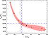 |
Fig. 6. Dereddened colors and effective temperatures for giant (red dots) and dwarfs (black dots). The best third-order polynomial fit is shown, along with 95% confidence and prediction bands indicated by strong and soft colors, respectively. We show the observed colors of OGLE-LMC-DPV-062 during main eclipse in five long-cycle phases as vertical lines, while the solid dashed line shows the average color and the horizontal line the upper limit for the donor temperature, viz., 10 111 ± 308 K (see text for details). |
In the analysis of overcontact or semidetached binary systems based solely on photometric time series and lacking spectroscopic data, the q-search method is widely used to estimate the mass ratio of the system. This technique is particularly reliable for eclipsing binaries showing total eclipses (Terrell & Wilson 2005), and might be considered an approximation for high-inclination binaries, although resulting uncertainties may still be underestimated. By applying this method, we obtained convergent solutions for a range of mass ratios defined as q = M2/M1, where subscripts 2 and 1 refer to the cooler and hotter components, respectively. We selected dataset 1 for this analysis, as it best represents the orbital light curve with minimal brightness attenuation due to disk obscuration of the primary star. The q search was conducted over the range q = 0.20 − 0.40, with a variable step size typically of 0.01. A mass ratio of q = 0.261 yielded the best agreement with the observed data (Fig. 7). This mass ratio is consistent with previous results for DPVs, where an average value of q = 0.23 ± 0.05 (standard deviation) has been reported (Mennickent et al. 2016). We notice that the minimum of the fourth-order polynomial fit is found at 0.271 ± 0.005, obtained with the bootstrapping technique and 1000 iterations. Considering the asymmetrical shape of the fit, we consider the mass ratio of q = 0.26 ± 0.04 to be the most reasonable value. From our analysis we also determined that the fits are sensitive to the adopted inclination and that the best fit is found at an inclination angle of about 78 degrees.
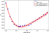 |
Fig. 7. Parameter S = Σ (O–C)2 for the fits done to the light curve of dataset 1, as a function of mass ratio. The best fourth-order polynomial fit is also shown along with a vertical line showing the minimum at q = 0.261. |
We calculated the stellar and orbital parameters by keeping the mass ratio fixed and starting with a donor temperature of 10 kK and then searching for the best fit of the light curve of dataset 1, varying the gainer temperature. The results were compared with the evolutionary track obtained with the MESA code (Section 4), with some mismatches being found that were solved by lowering the donor temperature and the overall system mass. The adopted parameters are listed in Table 3 and their errors are based on the estimates provided in Appendix A.
Datasets used in this paper.
Summary of stellar and orbital parameters and their formal errors.
3.4. Light curve models
In this section, we present our modeling of the light curve focused on OGLE-IV photometry, as the uncertainties associated with MACHO data are approximately an order of magnitude higher. To investigate photometric variability, the full dataset was partitioned into 20 subsamples, each representing consecutive phases of the long cycle (Table 2).
We calculated the mass transfer rate according to Eq. (2). To standardize the values of Ṁ we obtained, we referenced the minimum value, which was recorded at dataset 18. These values are displayed in Table 2. The normalized mass transfer rates calculated in this way have a mean value of 5.45× with a standard deviation of 4.29×, and maximum and minimum values of 16.25× and 1×. An uncertainty for Ṁ on the order of 25% was estimated considering the scatter of the fit to the long-term tendency discussed in Section 3.4. By contrast, the uncertainty obtained through error propagation may reach 40%. The variability of Ṁ is treated qualitatively in this paper and is not constrained by these limits.
The stellar and orbital parameters derived in the above section were held fixed for all datasets, allowing us to focus the analysis on the variability of the accretion disk properties. The full results from the light curve fitting are presented in Table 4. Parameter uncertainties were estimated from the 95% confidence bands of the fits of the parameters during the long-term cycle, discussed later in this section, they are consistent with uncertainties estimated from numerical trials of the parameters around the best-model values.
Light curve fit parameters for the data segments at the I band along with formal errors, mean, and standard deviation. Mean results are also given for the analysis of the BM and RM bands.
Orbital light curve fits for individual datasets are shown in Figs. B.3 and B.4 illustrating measurement uncertainties, typical orbital features, long-term variability, fit quality, and the corresponding visual representations of the system. Discrepancies beyond the formal errors of individual data points may reflect underestimated uncertainties or model limitations. For example, the model does not consider possible additional light sources. Furthermore, since some light curves span multiple orbital periods, long-term variations may also affect the fits. To mitigate this, we applied a low-degree sliding polynomial to each light curve segment and determined magnitudes at orbital phases 0.25 using the corresponding phase values from the polynomial fits (see Table 2).
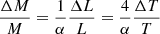
Our analysis reveals that the disk radius varies between 13.31 R⊙ and 17.77 R⊙, while the disk temperature ranges from 4788 K to 5830 K. The outer vertical thickness of the disk spans 2.48−5.37 R⊙, and the inner vertical thickness varies between 0.49 and 4.95 R⊙. The temperature of the hot spot is, on average, 2.21 ± 0.09 times higher than the surrounding disk, while the bright spot is 1.77 ± 0.10 times hotter than its surroundings.
The hot and bright spots are located at 323 3 ± 5
3 ± 5 7 and 56
 6 ± 5
6 ± 5 4, respectively, measured from the line connecting the stellar centers (from the donor to the gainer), in the direction of orbital motion. Their angular extents along the outer edge of the disk are 24
 9 ± 1
9 ± 1 4 for the hot spot and 50
 5 ± 6
5 ± 6 9 for the bright spot.
The MACHO B and R light curves show similar tendencies, but with much larger noise. We show the average values for their fits in Table 4.
We find that the mass transfer rate is maximum at the long cycle phase 0.5, coinciding with the minimum of the magnitude at orbital phase 0.25 and roughly with the minimum of the disk radius revealed by their fit function (Fig. 8). Most notably, the minimum brightness is found when the inner vertical disk extension is maximum, i.e., at a larger gainer occultation. This finding shows that in this system, the long cycle is mostly driven by cyclic occultations of the gainer by a disk of variable thickness.
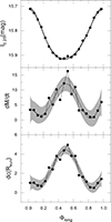 |
Fig. 8. Magnitude, normalized mass transfer rate and disk thickness at the central edge, as a function of the long-term cycle phase. Sixth-order polynomial fits along with the 95% confidence bands are shown. The parameters of these fits are given in Table 4. |
In addition, the angular positions of the hot and bright spots are constrained to well-defined regions during the cycle (Fig. 9). The average radius and temperature of the disk are consistent considering the fits for the I, RM and BM bandpasses.
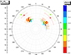 |
Fig. 9. Radial position and angular extension of hot spot (solid circles) and bright spot (squares) at different long-cycle phases. Colors indicate the normalized mass transfer rate. |
The correlation matrix confirms the previous results and indicates that no parameter degeneracies are present (Fig. B.5). We considered as statistically significant those correlations with a p value equal to or under 0.05, i.e., with a probability equal or lower than 0.05 that the correlation (or anticorrelation) is nonexistent. The analysis reveals that θbs and λhs correlate with aT and system brightness, respectively. The parameters Ahs and Abs are anticorrelated with de. The matrix also confirms the strong correlation between the disk’s inner edge thickness and the system brightness.
Interestingly, the positions of the main and secondary eclipses, measured with Gaussian fits, follow systematic tendencies with the long-term cycle. These changes are reproduced by the models and could indicate changes in the photo-center, as is suggested by the behavior of the hot and bright spots during the long cycle (Fig. 10).
 |
Fig. 10. Top: Minima of Gaussian fits to the main and secondary eclipses for datasets of Table 2. Bottom: Position of the hot and bright spots during the long cycle and the best third-order polynomial fits, along with their 95% prediction and confidence bands. |
4. The evolutionary stage
We simulated the evolution of the binary system OGLE-LMC-DPV-062 with MESA following Rosales et al. (2019). The simulation initiates at the zero-age main sequence (ZAMS) under a quasi-conservative mass transfer regime, which is maintained until the helium-4 mass fraction in the donor star’s core (X4He, c) drops below 0.2. To identify the optimal model, we extensively explored the parameter space: the initial orbital period (Pi, o) was varied from 1.0 to 6.0 days (steps of 0.1 d); the initial stellar masses were explored with Mi, d ranging from 6.0 to 9.0 M⊙ and, conversely, Mi, g from 9.0 to 6.0 M⊙ (steps of 0.1 M⊙); and a metallicity of Z = 0.006 was fixed, consistent with the assumed chemical composition of the LMC. Key nonconservative mass loss parameters were optimized: the α parameter (fraction of mass lost from the donor as a fast Jeans-type wind) was explored from 9 × 10⁻⁸ to 9 × 10⁻¹, and the β parameter (fraction of mass ejected as a fast isotropic wind from the vicinity of the accretor after reemission) was optimized, maintaining β > α. To independently modulate the envelope structure and evolutionary rate of both stellar components, we varied the mixing length parameter (αML), which governs the efficiency of convective energy transport in MESA via the mixing length theory (MLT). αML is defined as the ratio between the mixing length and the star’s pressure scale height. A high αML (e.g., ≥1.0) implies efficient convection (near-adiabatic gradient), while a very low value simulates inefficient convection, significantly affecting the stellar radius and evolution. As a reference, αML varies systematically in the range of 1.7–2.4 for stars of solar metallicity (Magic et al. 2015). However, uncertainties remain for stars quite different from the Sun (e.g., low metallicity, evolved giants, very low or high mass), limiting the predictive reliability of 1D evolutionary models in those regimes. In this study, we varied the αML value from 0.0001 to 4.0 for the donor star, keeping the value for the gainer at 1.8.
The determination of the best-fitting initial parameters was achieved through a rigorous minimization analysis using the chi-squared (χ2) statistic. This method compares the theoretical outputs from the MESA simulations with the observed physical parameters. To refine the fitting process, a weighted χ2 function was implemented, whereby individual contributions from the observed parameters were scaled using weight factors (wi), with certain observables (such as mass and orbital period) being prioritized over others (such as luminosity and temperature).
The best model, which yielded the lowest chi-squared value of χ2 = 0.1486, converged with the following initial conditions: a donor mass of Mi, d = 6.3 M⊙, an accretor mass of Mi, g = 5.9 M⊙, and an initial orbital period of Pi, o = 2.5 d. The corresponding mass transfer parameters were α = 8 × 10⁻⁵ M⊙/yr and β = 1 × 10⁻⁴ (the δ mode was set to 0). The donor αML parameter required for convergence was 4.0. This value is high for the standards, and could be influenced by the fact that the upper levels of the donor atmosphere are being affected by the mass transfer. We notice that lower values fail in reproducing well the position of the donor in the luminosity–temperature diagram. The best fit model at the present age (47.92 Myr) is characterized by Mg = 9.34 M⊙, Md = 2.83 M⊙, Rg = 5.16 R⊙, Rd = 10.21 R⊙, Tg = 26 662 K, and Md = 6973 K.
The evolutionary tracks of the gainer and donor are shown in Fig. 11, with labels indicating the evolutionary stages described in Table 5. Variations in the central helium and hydrogen abundances reflect hydrogen depletion and helium enrichment in the cores of both stars. However, at the current evolutionary stage, the gainer exhibits a rejuvenation effect, resulting from the increase in its central hydrogen content supplied by the donor during mass transfer, with the accreted hydrogen being efficiently mixed from the surface into the stellar interior (see Fig. 11).
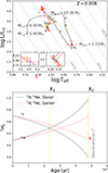 |
Fig. 11. Top: evolutionary tracks for the best quasi-conservative model. Blue dots with error bars are the observed values and the triangles are the model’s values. The labels correspond to the evolutionary stages given in Table 5. Bottom: central abundance of hydrogen and helium for the gainer and donor. X1 corresponds to the inversion of the 1H/4He ratio and X2 to the current stage. |
Evolutionary stages of DPV062.
5. Discussion
Before we proceed with the interpretation of our results, it is important to be aware of the limitations of our model. A key simplification is our focus exclusively on circumstellar material within the disk, overlooking any light contributions originating from regions above or below the disk plane. Additionally, we have assumed that the gainer is surrounded by an accretion disk, disregarding other potential light sources such as jets, winds, and outflows. Nonetheless, the model allows for the possibility of accounting for variations in disk emissivity that are dependent on azimuthal position through the inclusion of two disk spots. Despite these constraints, and drawing on prior research on algols with disks, our model likely captures the principal light sources for the continuum light. This is evidenced by the close correspondence between the model light curve and the orbital and long-term light curves over the span of 32.3 years of observation (the time covered by the I-band OGLE time series). This finding that the long cycle of OGLE-LMC-DPV-062 is a consequence of its variable accretion disk is consistent with recent claims that DPV cycles represent the disk’s cyclic structural changes (e.g., Garcés et al. 2018, 2025). In this section, we discuss the evolutionary stage of the binary and also provide a test for the magnetic dynamo hypothesis of the long-term cycle.
5.1. The disk size and mass transfer rate
We ran evolutionary models and found the one that best reproduces the present state of the system. Although the match is not perfect, we can certainly infer that the system is a product of the evolution of a stellar pair that experiences strong mass transfer in a semidetached stage with Roche lobe overflow (RLOF).
The fractional radius of the gainer is R1/a = 0.143. This value reveals a tangential impact system, where the gas stream hits the gainer almost tangentially, provoking the formation of an accretion disk (Lubow & Shu 1975).
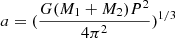
In principle, the disk can be stable until the last nonintersecting orbit defined by the tidal radius (Paczynski 1977; Warner 1995, Eq. (2.61))
 (5)
(5)
We get Rt/aorb = 0.476, or Rt = 17.10 R⊙. We observe that during all observing epochs (except set 6 when is 17.8) the disk outer radius keeps inside the volume defined by the tidal radius. This discards the possible influences of tidal forces in shaping the outer parts of the disk.
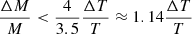
The value of the mass transfer rate of 9.7 × 10⁻⁵ M⊙/yr must be consistent with the constancy of the orbital period. For a binary system ongoing conservative mass transfer, we should expect a change in the orbital period of (Huang 1963)
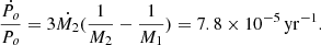 (6)
(6)
This means a change of 5.42 × 10⁻⁴ days per year, or 0.01750 days during the whole observing window. This is almost 45 times larger than the period error of 0.000393 days. As is not observed, the actual mass transfer rate is much smaller than 9.7 × 10⁻⁵ M⊙/yr or systemic mass loss is important for the system angular momentum balance. The mass transfer rate compatible with the constancy of the orbital period should be lower than 2.2 × 10⁻⁶ M⊙/yr. In the case of important systemic mass loss in the past, the system total mass should be smaller than calculated.
In principle, mass loss in a semidetached binary undergoing RLOF can occur through the outer Lagrangian points L2 and L3, via stellar winds, or even through a jet of material directed roughly perpendicular to the orbital plane. These mechanisms are either theoretically predicted (Scherbak et al. 2025) or have been observationally reported in some DPVs (Mennickent et al. 2012; Harmanec et al. 1996). However, the evolutionary pathways of Roche-lobe overflowing binaries remain highly uncertain, as key processes such as the efficiency of accretion onto the gainer and the resulting spin-up are still poorly constrained. Consequently, modeling nonconservative evolution during episodes of systemic mass loss remains a major theoretical challenge (Marchant & Bodensteiner 2024), although recent results indicate predominantly conservative cases in a subset of 16 Be+sdOB binaries (Lechien et al. 2025).
5.2. Test for the magnetic dynamo model
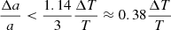
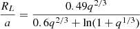
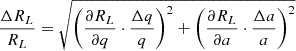
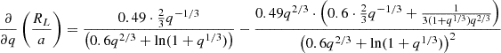
Assuming that the magnetic dynamo mechanism acting on the donor star is the origin of the long cycle, it is possible to estimate the theoretical duration of this cycle from the relations between the Keplerian period (PKep), the convective velocity (vc), and the Rossby number (Ro). The latter can be evaluated, following Schleicher & Mennickent (2017), as
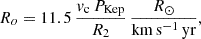
where R2 is the radius of the donor star. In addition, the Rossby number is linked to the dynamo number (D) through  , so that the duration of the magnetic cycle acting on the donor can be estimated from (Schleicher & Mennickent 2017, and references therein):

where γ has typical values of between 1/3 and 5/6 and the equation shows the link between the rotational period of a single star (assumed here to be equal to the orbital period) and the cycle length of its magnetic dynamo (Soon et al. 1993; Baliunas et al. 1996).
Following this approach, and using the physical parameters of the donor obtained from the best evolutionary model computed with MESA, we can trace the temporal evolution of the ratio Pcycle/Porb as the radius, luminosity, and stellar mass of the donor change during the RLOF phase.
In Fig. 12 we note a good agreement between the theoretical value of Pcycle/Porb and the observed ratio, Plong/Porb. This fit is achieved by adopting a value of γ = 0.27 ± 0.01, slightly below than the γ = 0.31 predicted for DPVs, but within the expected range for active stars (∼0.25 − 0.83; Schleicher & Mennickent 2017).
 |
Fig. 12. Top: mass-transfer rate and evolution of the donor star mass. Bottom: evolution of the theoretical value of Pcycle/Porb considering γ = 0.27 ± 0.01 (blue region), together with the estimated dynamo number. The horizontal line shows the observed relation Plong/Porb = 33.2. In both panels, the vertical line indicates the age, according to the best MESA evolutionary model, at which the system reaches an orbital period of |

We confirm a pronounced variation in the donor’s dynamo number during the mass-transfer episode as reported by San (2019). These variations are linked to structural changes in the donor star, particularly in its radius and rotational velocity. It is therefore plausible that the conditions required for a magnetic dynamo operate only within a limited time window during the overall mass-transfer phase, a period compatible with the observed DPV γ values. However, the observation that the long-term cycle could change or even disappear on very short timescales, as occurs in AU Mon (Celedón et al. 2025), indicates that other mechanisms beside changes in the internal donor structure influence the long-term cycles.
5.3. Comparison with other DPVs
OGLE-LMC-DPV-062 shows stellar parameters in the range exhibited by other DPVs. In terms of the long-term cycle, it shows a behavior similar to OGLE-BLG-ECL-157529, OGLE-LMC-ECL-14413, and RX Cas; an increase in the mass transfer rate produces a thicker disk and a fainter system (Mennickent & Djurašević 2021; Mennickent et al. 2022, 2025). However, in OGLE-LMC-DPV-097 the disk radius is the primary factor governing the brightness at both maximum and minimum light (Garcés et al. 2018), whereas in OGLE-LMC-DPV-065, which shows a double-hump long-term light curve, the disk central thickness decreases at maximum brightness, and both the disk temperature and radius display complex cyclic variations (Mennickent & Djurašević 2025). It is clear that the behavior is not necessarily the same for all DPVs and that more research is needed to understand how the disk reacts to changes in the mass transfer rate.
6. Conclusion
We have analyzed the remarkable long-term light curve of the DPV system OGLE-LMC-DPV-062, covering a timespan of 32.3 years, and have obtained, for the first time, a physical description of the whole system. Our model successfully reproduces the overall I-band variability, accounting for both the orbital modulation with a period of 6 90 and the long-term DPV cycle of 229
 7.
7.
We find that the system consists of a B-type main-sequence star, of approximately spectral type B1.5, accreting matter from a cooler A9-F0 type giant, according to the classification scheme of Harmanec (1988). Our study traces the system’s evolutionary path, indicating that it is currently undergoing an episode of rapid mass transfer as the donor fills its Roche lobe. We estimated the fundamental stellar parameters of the binary. The components have masses of 10.36 ± 1.14 M⊙ and 2.73 ± 0.30 M⊙, radii of 5.14 ± 0.98 R⊙ and 9.71 ± 0.56 R⊙, and effective temperatures of 24 400 ± 2400 K and 7100 ± 700 K, respectively. The orbital separation is 35.9 ± 1.4 R⊙, and the surface gravities are log g = 4.03 ± 0.17 and 2.90 ± 0.07. These estimates should be treated with caution, since the possibility of nonconservative mass transfer, along with related uncertainties not considered here, cannot be excluded.
Our model incorporates the contribution of an accretion disk with an average radius of 14.5 R⊙ and includes two hot shock regions at the disk’s outer edge. We detect substantial variations in the disk’s vertical structure, suggesting that turbulence and large-scale motions may play a role in sustaining its thickness.
We find that the normalized mass-transfer rate varies in accordance with the long-term cycle, reaching at maximum 16 times its minimum value, when the system’s total brightness is at its minimum. At this stage, the disk attains its greatest vertical thickness at the inner edge, of almost 5 R⊙, obscuring a larger portion of the gainer. In our model, the disk’s variability is primarily expressed through changes in vertical extension, while its radius and the temperature at the outer rim exhibit only minor variations throughout the long-term cycle. Additionally, hot and bright spots are present on the disk surface at roughly constant azimuths, located opposite the donor star. Although no direct evidence of magnetism is found, a good match is observed between the prediction of the magnetic dynamo model of Schleicher & Mennickent (2017) and the observed ratio between the orbital and long-term cycle periods.
Acknowledgments
We thank the anonymous referee for the useful comments and suggestions on the first version of this manuscript. We acknowledge support by the ANID BASAL project Centro de Astrofísica y Tecnologías Afines ACE210002 (CATA). This work has been co-funded by the National Science Centre, Poland, grant No. 2022/45/B/ST9/00243.
References
- Alcock, C., Allsman, R. A., Alves, D., et al. 1997, ApJ, 486, 697 [NASA ADS] [CrossRef] [Google Scholar]
- Alcock, C., Allsman, R. A., Alves, D. R., et al. 1999, PASP, 111, 1539 [NASA ADS] [CrossRef] [Google Scholar]
- Albright, G. E., & Richards, M. T. 1996, ApJ, 459, L99 [NASA ADS] [Google Scholar]
- Atwood-Stone, C., Miller, B. P., Richards, M. T., Budaj, J., & Peters, G. J. 2012, ApJ, 760, 134 [NASA ADS] [CrossRef] [Google Scholar]
- Baliunas, S. L., Nesme-Ribes, E., Sokoloff, D., & Soon, W. H. 1996, ApJ, 460, 848 [Google Scholar]
- Bisikalo, D. V., Harmanec, P., Boyarchuk, A. A., Kuznetsov, O. A., & Hadrava, P. 2000, A&A, 353, 1009 [NASA ADS] [Google Scholar]
- Brož, M., Mourard, D., Budaj, J., et al. 2021, A&A, 645, A51 [EDP Sciences] [Google Scholar]
- Celedón, L., Mennickent, R. E., Barría, D., Garcés, J., & Jurković, M. 2025, A&A, 700, A217 [NASA ADS] [CrossRef] [EDP Sciences] [Google Scholar]
- Claret, A. 2000, A&A, 363, 1081 [NASA ADS] [Google Scholar]
- Dennis, J. E., & Torczon, V. 1991, SIAM J. Optim., 1, 448 [Google Scholar]
- Djurašević, G. 1992, Ap&SS, 196, 267 [Google Scholar]
- Djurašević, G. 1996, Ap&SS, 240, 317 [Google Scholar]
- Djurašević, G., Vince, I., & Atanacković, O. 2008, AJ, 136, 767 [Google Scholar]
- Djurašević, G., Latković, O., Vince, I., & Cséki, A. 2010, MNRAS, 409, 329 [CrossRef] [Google Scholar]
- Eggleton, P. P. 1983, ApJ, 268, 368 [Google Scholar]
- Eggenberger, P., Ekström, S., Georgy, C., et al. 2021, A&A, 652, A137 [NASA ADS] [CrossRef] [EDP Sciences] [Google Scholar]
- Eggleton, P. Evolutionary Processes in Binary and Multiple Stars (Cambridge, UK: Cambridge University Press) [Google Scholar]
- Foster, G. 1996, AJ, 112, 1709 [NASA ADS] [CrossRef] [Google Scholar]
- Gaposchkin, S. 1944, ApJ, 100, 230 [NASA ADS] [CrossRef] [Google Scholar]
- Garcés, L. J., Mennickent, R. E., Djurašević, G., Poleski, R., & Soszyński, I. 2018, MNRAS, 477, L11 [CrossRef] [Google Scholar]
- Garcés, J., Mennickent, R. E., Petrovíc, J., et al. 2025, A&A, 701, A90 [NASA ADS] [CrossRef] [EDP Sciences] [Google Scholar]
- Głowacki, M., Soszyński, I., Udalski, A., et al. 2024, AcA, 74, 241 [Google Scholar]
- Graczyk, D., Soszyński, I., Poleski, R., et al. 2011, AcA, 61, 103 [Google Scholar]
- Guinan, E. F. 1989, Space Sci. Rev., 50, 35 [NASA ADS] [CrossRef] [Google Scholar]
- Harmanec, P. 1988, Bull. Inst. Czechoslovakia, 39, 329 [Google Scholar]
- Harmanec, P., Morand, F., Bonneau, D., et al. 1996, A&A, 312, 879 [Google Scholar]
- Hill, G., Harmanec, P., Pavlovski, K., et al. 1997, A&A, 324, 965 [NASA ADS] [Google Scholar]
- Huang, S.-S. 1963, ApJ, 138, 471 [NASA ADS] [CrossRef] [Google Scholar]
- Iwanek, P., Soszyński, I., & Kozłowski, S. 2021, ApJ, 919, 99 [NASA ADS] [CrossRef] [Google Scholar]
- Kaigorodov, P. V., Bisikalo, D. V., & Kurbatov, E. P. 2017, Astron. Rep., 61, 639 [NASA ADS] [CrossRef] [Google Scholar]
- Koubsky, P., Harmanec, P., Bozic, H., et al. 1998, Hvar Obs. Bull., 22, 17 [Google Scholar]
- Lang, K. 1993, Astronomy, 21, 95 [Google Scholar]
- Lechien, T., de Mink, S. E., Valli, R., et al. 2025, ApJ, 990, L51 [Google Scholar]
- Lomax, J. R., Hoffman, J. L., Elias, N. M., Bastien, F. A., & Holenstein, B. D. 2012, ApJ, 750, 59 [CrossRef] [Google Scholar]
- Lorenzi, L. 1980, A&A, 85, 342 [NASA ADS] [Google Scholar]
- Lubow, S. H., & Shu, F. H. 1975, ApJ, 198, 383 [NASA ADS] [CrossRef] [Google Scholar]
- Magic, Z., Weiss, A., & Asplund, M. 2015, A&A, 573, A89 [NASA ADS] [CrossRef] [EDP Sciences] [Google Scholar]
- Marchant, P., & Bodensteiner, J. 2024, ARA&A, 62, 21 [NASA ADS] [CrossRef] [Google Scholar]
- Mennickent, R. E. 2017, Serb. Astron. J., 194, 1 [NASA ADS] [CrossRef] [Google Scholar]
- Mennickent, R. E., & Djurašević, G. 2013, MNRAS, 432, 799 [NASA ADS] [CrossRef] [Google Scholar]
- Mennickent, R. E., & Djurašević, G. 2021, A&A, 653, A89 [NASA ADS] [CrossRef] [EDP Sciences] [Google Scholar]
- Mennickent, R. E., & Djurašević, G. 2025, A&A, 698, A56 [NASA ADS] [CrossRef] [EDP Sciences] [Google Scholar]
- Mennickent, R. E., Pietrzyński, G., Diaz, M., & Gieren, W. 2003, A&A, 399, 47 [Google Scholar]
- Mennickent, R. E., Kołaczkowski, Z., Michalska, G., et al. 2008, MNRAS, 389, 1605 [NASA ADS] [CrossRef] [Google Scholar]
- Mennickent, R. E., Kołaczkowski, Z., Djurasevic, G., et al. 2012, MNRAS, 427, 607 [NASA ADS] [CrossRef] [Google Scholar]
- Mennickent, R. E., Otero, S., & Kołaczkowski, Z. 2016, MNRAS, 455, 1728 [NASA ADS] [CrossRef] [Google Scholar]
- Mennickent, R. E., Garcés, J., Djurašević, G., et al. 2020a, A&A, 641, A91 [NASA ADS] [CrossRef] [EDP Sciences] [Google Scholar]
- Mennickent, R. E., Djurašević, G., Vince, I., et al. 2020b, A&A, 642, A211 [NASA ADS] [CrossRef] [EDP Sciences] [Google Scholar]
- Mennickent, R. E., Djurašević, G., Petrović, J., et al. 2022, A&A, 666, A51 [NASA ADS] [CrossRef] [EDP Sciences] [Google Scholar]
- Mennickent, R. E., Djurašević, G., Rosales, J. A., et al. 2025, A&A, 693, A217 [NASA ADS] [CrossRef] [EDP Sciences] [Google Scholar]
- Mourard, D., Brož, M., Nemravová, J. A., et al. 2018, A&A, 618, A112 [NASA ADS] [CrossRef] [EDP Sciences] [Google Scholar]
- Nugis, T., & Lamers, H. J. G. L. M. 2000, A&A, 360, 227 [NASA ADS] [Google Scholar]
- Paczyński, B. 1971, ARA&A, 9, 183 [Google Scholar]
- Paczynski, B. 1977, ApJ, 216, 822 [CrossRef] [Google Scholar]
- Pawlak, M., Graczyk, D., Soszyński, I., et al. 2013, Acta Astron., 63, 323 [NASA ADS] [Google Scholar]
- Pawlak, M., Soszyński, I., Udalski, A., et al. 2016, Acta Astronomika, 66, 421 [Google Scholar]
- Paxton, B., Bildsten, L., Dotter, A., et al. 2011, ApJS, 192, 3 [Google Scholar]
- Paxton, B., Cantiello, M., Arras, P., et al. 2013, ApJS, 208, 4 [Google Scholar]
- Paxton, B., Marchant, P., Schwab, J., et al. 2015, ApJS, 220, 15 [Google Scholar]
- Paxton, B., Schwab, J., Bauer, E. B. 2018, ApJS, 234, 34 [NASA ADS] [CrossRef] [Google Scholar]
- Poleski, R., Soszyński, I., Udalski, A., et al. 2010, Acta Astron., 60, 179 [NASA ADS] [Google Scholar]
- Ritter, H. 1988, A&A, 202, 93 [NASA ADS] [Google Scholar]
- Rojas, García G., Mennickent, R., Iwanek, P., et al. 2021, ApJ, 922, 30 [Google Scholar]
- Rosales, Guzmán J. A., Mennickent R. E., Djurašević G., Araya I., Curé M., 2018, MNRAS, 476, 3039 [Google Scholar]
- Rosales, J. A., Mennickent, R. E., Schleicher, D. R. G., & Senhadji, A. A. 2019, MNRAS, 483, 862 [Google Scholar]
- Rosales, J. A., Petrović, J., Mennickent, R. E., Schleicher, D. R. G., Djurašević, G., & Leigh, N. W. C. 2024, A&A, 689, A154 [NASA ADS] [CrossRef] [EDP Sciences] [Google Scholar]
- San, Martín-Pérez R. I., Schleicher D. R. G., Mennickent R. E., Rosales J. A., 2019, Boletín de la Asociación Argentina de Astronomía, 61, 107 [Google Scholar]
- Scherbak, P., Lu, W., & Fuller, J. 2025, ApJ, 990, 172 [Google Scholar]
- Schleicher, D. R. G., & Mennickent, R. E. 2017, A&A, 602, A109 [NASA ADS] [CrossRef] [EDP Sciences] [Google Scholar]
- Skowron, D. M., Skowron, J., Udalski, A., et al. 2021, ApJS, 252, 23 [Google Scholar]
- Stellingwerf, R. F. 1978, ApJ, 224, 953 [Google Scholar]
- Soon, W. H., Baliunas, S. L., & Zhang, Q. 1993, ApJ, 414, L33 [Google Scholar]
- Terrell, D., & Wilson, R. E. 2005, Ap&SS, 296, 221 [NASA ADS] [CrossRef] [Google Scholar]
- Udalski, A., Szymański, M. K., & Szymański, G. 2015, Acta Astron., 65, 1 [NASA ADS] [Google Scholar]
- Vink, J. S., de Koter, A., & Lamers, H. J. G. L. M. 2001, A&A, 369, 574 [NASA ADS] [CrossRef] [EDP Sciences] [Google Scholar]
- von Zeipel, H. 1924, MNRAS, 84, 702 [Google Scholar]
- Warner, B. 1995, Cataclysmic Variable Stars, Cambridge Astrophysics Series, 28 [Google Scholar]
- Wilson, R. E., & Devinney, E. J. 1971, ApJ, 166, 605 [Google Scholar]
- Zechmeister, M., & Kürster, M. 2009, A&A, 496, 577 [CrossRef] [EDP Sciences] [Google Scholar]
Appendix A: Error estimates
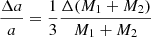
We estimate the errors of mass, radius and orbital separation assuming an uncertainty in the temperature and using an analytical approach. The luminosity follows the Stefan-Boltzmann law:
 (A.1)
(A.1)
where R is the radius of the star, σ is the Stefan-Boltzmann constant, and T is the effective temperature. Now, an error in the temperature, ΔT, affects the luminosity due to the dependence L ∝ T4. If we make an error ΔT in measuring the effective temperature of the star, the relative error in the luminosity will be:
 (A.2)
(A.2)
Given that for a main sequence star L ∝ Mα, an error in the luminosity, ΔL, translates into an error in the mass, ΔM, as follows:
 (A.3)
(A.3)
If we use α≈ 3.5 for a main sequence star, and consider that for a giant star the exponent should be larger because of the increasing radius, the relative error in the mass of the donor would be:
 (A.4)
(A.4)
On the other hand, the orbital separation in a binary system is given by Kepler’s third law:
 (A.5)
(A.5)
An error in the stellar masses affects the orbital separation as follows:
 (A.6)
(A.6)
Assuming the relative error is similar for both stars, we can write:
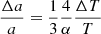 (A.7)
(A.7)
For α > 3.5:
 (A.8)
(A.8)
From the above equations, and assuming a temperature uncertainty of 10%, we get masses with uncertainty of less than 11% and orbital separation with uncertainty of less than 4%.
To calculate the error in the radius of the giant star filling its Roche lobe, we need to consider how the errors in the mass ratio (q = M1/M2) and the orbital separation (a) affect the error in the Roche lobe radius (RL).
Recall that the Roche lobe radius is given by the empirical Eggleton formula:
 (A.9)
(A.9)
To find the error in RL (the Roche lobe radius, which will approximately be the radius of the giant star), we applied the formula for error propagation. This allows us to calculate the error in RL as a function of the errors in q and a.
Since RL depends on two variables, q and a, the error in RL, denoted as ΔRL, can be computed using the following error propagation formula:
 (A.10)
First we calculate the partial derivative with respect to q:
 (A.11)
Then, we calculate the partial derivative with respect to a. The dependence of RL on a is straightforward, as RL ∝ a. Thus:
 (A.12)
For q = 0.26 with an associated error of 0.04, and assuming a 4% relative error in the orbital separation, we obtain a relative error of 4.1% for the Roche Lobe radius, which also corresponds to the donor star’s radius.
If the gainer follows a mass-radius relationship M ∝ Rβ with β between 0.57 and 0.7, we get the fractional error in the gainer radius less than 1.75 times the fractional error in the gainer mass. If this last is 11%, then the gainer fractional radius uncertainty is less than 19%.
Finally, the surface gravity in solar units is given by:
 (A.13)
where log g⊙ is the solar surface gravity. The error is given by:
 (A.14)
Using the fractional errors quoted above, we derive the errors for log g given in Table 3, viz. 4% por the gainer and 2% for the donor.
Appendix B: Additional material
 |
Fig. B.1. MACHO BM (colored) and RM light curves. |
 |
Fig. B.2. MACHO BM-RM color versus orbital and long-term cycle phases. |
 |
Fig. B.3. Orbital light curve fits for individual datasets 1-10. |
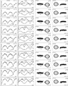 |
Fig. B.4. Orbital light curve fits for individual datasets 11-20. |
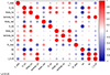 |
Fig. B.5. Correlation matrix for the fit’s parameters showing with asterisks those cases with p-value equal or under 0.05. The right vertical color scale shows the correlation coefficient. |
Coefficients for the fits shown in Fig.8.
All Tables
Light curve fit parameters for the data segments at the I band along with formal errors, mean, and standard deviation. Mean results are also given for the analysis of the BM and RM bands.
All Figures
|
Fig. 1. Section of the OGLE I-band light curve of OGLE-LMC-DPV-062. Colors indicate different orbital phases. |
| In the text | |
|
Fig. 2. WWZ transform showing a strong signal around 230 days. The orbital period was removed before the analysis. |
| In the text | |
|
Fig. 3. Orbital light curve colored with the long-term cycle phase of the data. Magnitudes subtracting the minimum magnitude of the respective dataset are shown in the graph below. |
| In the text | |
|
Fig. 4. I-band magnitudes taken at orbital phases [0.2–0.3; up] and [0.9–1.1; down] phased with the long-term cycle phase. |
| In the text | |
|
Fig. 5. MACHO BM − RM color versus orbital and long-term cycle phases. |
| In the text | |
|
Fig. 6. Dereddened colors and effective temperatures for giant (red dots) and dwarfs (black dots). The best third-order polynomial fit is shown, along with 95% confidence and prediction bands indicated by strong and soft colors, respectively. We show the observed colors of OGLE-LMC-DPV-062 during main eclipse in five long-cycle phases as vertical lines, while the solid dashed line shows the average color and the horizontal line the upper limit for the donor temperature, viz., 10 111 ± 308 K (see text for details). |
| In the text | |
|
Fig. 7. Parameter S = Σ (O–C)2 for the fits done to the light curve of dataset 1, as a function of mass ratio. The best fourth-order polynomial fit is also shown along with a vertical line showing the minimum at q = 0.261. |
| In the text | |
|
Fig. 8. Magnitude, normalized mass transfer rate and disk thickness at the central edge, as a function of the long-term cycle phase. Sixth-order polynomial fits along with the 95% confidence bands are shown. The parameters of these fits are given in Table 4. |
| In the text | |
|
Fig. 9. Radial position and angular extension of hot spot (solid circles) and bright spot (squares) at different long-cycle phases. Colors indicate the normalized mass transfer rate. |
| In the text | |
|
Fig. 10. Top: Minima of Gaussian fits to the main and secondary eclipses for datasets of Table 2. Bottom: Position of the hot and bright spots during the long cycle and the best third-order polynomial fits, along with their 95% prediction and confidence bands. |
| In the text | |
|
Fig. 11. Top: evolutionary tracks for the best quasi-conservative model. Blue dots with error bars are the observed values and the triangles are the model’s values. The labels correspond to the evolutionary stages given in Table 5. Bottom: central abundance of hydrogen and helium for the gainer and donor. X1 corresponds to the inversion of the 1H/4He ratio and X2 to the current stage. |
| In the text | |
|
Fig. 12. Top: mass-transfer rate and evolution of the donor star mass. Bottom: evolution of the theoretical value of Pcycle/Porb considering γ = 0.27 ± 0.01 (blue region), together with the estimated dynamo number. The horizontal line shows the observed relation Plong/Porb = 33.2. In both panels, the vertical line indicates the age, according to the best MESA evolutionary model, at which the system reaches an orbital period of |
| In the text | |
|
Fig. B.1. MACHO BM (colored) and RM light curves. |
| In the text | |
|
Fig. B.2. MACHO BM-RM color versus orbital and long-term cycle phases. |
| In the text | |
|
Fig. B.3. Orbital light curve fits for individual datasets 1-10. |
| In the text | |
|
Fig. B.4. Orbital light curve fits for individual datasets 11-20. |
| In the text | |
|
Fig. B.5. Correlation matrix for the fit’s parameters showing with asterisks those cases with p-value equal or under 0.05. The right vertical color scale shows the correlation coefficient. |
| In the text | |
Current usage metrics show cumulative count of Article Views (full-text article views including HTML views, PDF and ePub downloads, according to the available data) and Abstracts Views on Vision4Press platform.
Data correspond to usage on the plateform after 2015. The current usage metrics is available 48-96 hours after online publication and is updated daily on week days.
Initial download of the metrics may take a while.