| Issue |
A&A
Volume 709, May 2026
|
|
|---|---|---|
| Article Number | A112 | |
| Number of page(s) | 12 | |
| Section | Stellar structure and evolution | |
| DOI | https://doi.org/10.1051/0004-6361/202659031 | |
| Published online | 12 May 2026 | |
Two hot pre-white dwarfs inside the red giant branch planetary nebula Pa 13
Double-core evolution or common-envelope-induced rejuvenation
1
Zentrum für Astronomie der Universität Heidelberg, Landessternwarte, Königstuhl 12, D-69117 Heidelberg, Germany
2
Instituto de Astrofísica de Canarias, E-38205 La Laguna, Tenerife, Spain
3
Departamento de Astrofísica, Universidad de La Laguna, E-38206 La Laguna, Tenerife, Spain
4
Department of Physics and Astronomy, Valparaiso University, Valparaiso, IN 46383, USA
5
Instituto de Astrofísica de La Plata, UNLP-CONICET, La Plata, 1900 Buenos Aires, Argentina
6
Institut für Physik und Astronomie, Universität Potsdam, Haus 28, Karl-Liebknecht-Str. 24/25, D-14476 Potsdam-Golm, Germany
7
Department of Astronomy, University of Geneva, Chemin d’Ecogia 16, 1290 Versoix, Switzerland
★ Corresponding author: This email address is being protected from spambots. You need JavaScript enabled to view it.
Received:
19
January
2026
Accepted:
16
March
2026
Abstract
The close binary central stars of planetary nebulae (PNe) offer a unique window for investigating the conditions that immediately follow the ejection of a common envelope (CE). Double-eclipsing and double-lined double systems are particularly valuable as they provide minimally model-dependent constraints on fundamental binary parameters. In this context, we report that the nucleus of Pa 13 (P = 0.3988 d) belongs to this rare class of systems and we present a comprehensive analysis of its double-degenerate binary. We performed a two-component nonlocal thermodynamic equilibrium spectral analysis based on phase-resolved X-shooter spectroscopy, multiband light-curve modeling, spectral energy distribution fitting, and a kinematic analysis. Both stars are found to be hot pre-white dwarfs, with Star 1 being cooler but larger (Teff = 50.0 kK, R = 0.40 R⊙) than Star 2 (Teff = 75.0 kK, R = 0.16 R⊙). The weakness of the spectral lines of Star 2 made both the atmospheric and radial velocity (RV) analyses challenging, and we uncovered a strong sensitivity of the assumed surface ratio to its derived RV curve. However, the RV curve and Kiel mass of Star 1 (M1 = 0.41 ± 0.02 M⊙) could be determined precisely, which allowed for a dynamical mass determination of Star 2 (M2 = 0.39 ± 0.04 M⊙). Moreover, we uncovered that Pa 13 exhibits a small but significant orbital eccentricity (e = 0.02 ± 0.01), which makes it only the second post-CE binary central star with a measured eccentricity. Our kinematic analysis shows that Pa 13 belongs to the Galactic halo, implying a system age of ≈11 Gyr. We conclude that Pa 13 provides the strongest evidence so far that PNe can be observed around post-red giant branch stars. Immediately after the CE ejection, Star 1 likely still filled its Roche lobe, which suggests that Pa 13 is a more evolved, detached descendant of over-contact double-degenerate systems such as Hen 2-428. Since the mass ratio of Pa 13 is close to unity, the system may have formed through double-core CE evolution. Alternatively, there must exist an efficient CE-induced rejuvenation mechanism capable of reheating the cool white dwarf in the binary, as already indicated by the Hen 2-428 system.
Key words: stars: atmospheres / binaries: close / binaries: eclipsing / binaries: spectroscopic
© The Authors 2026
 Open Access article, published by EDP Sciences, under the terms of the Creative Commons Attribution License (https://creativecommons.org/licenses/by/4.0), which permits unrestricted use, distribution, and reproduction in any medium, provided the original work is properly cited.
This article is published in open access under the Subscribe to Open model. This email address is being protected from spambots. You need JavaScript enabled to view it. to support open access publication.
1. Introduction
The study of close double-degenerate binaries is of considerable importance as these systems serve as powerful sources of gravitational waves (Evans et al. 1987; Lipunov et al. 1987; Hils et al. 1990; Nelemans et al. 2001a; Burdge et al. 2019; Li et al. 2020), and contribute to our understanding of the progenitors of Type Ia supernovae (Webbink 1984) and the origin of hyper-velocity stars (Neunteufel et al. 2019; Shen 2025). Moreover, double degenerates constitute essential laboratories for investigating close binary evolution, including the common envelope (CE) phase (Nelemans & Tout 2005; Nelemans et al. 2025). Beyond their role as potential progenitors of thermonuclear supernovae, double-degenerate mergers may also give rise to ultramassive white dwarfs (WDs, Wu et al. 2022), highly magnetic WDs García-Berro et al. (2012), and a variety of other exotic stars (Zhang & Jeffery 2012b,a; Werner & Rauch 2015; Kawka et al. 2020; Dorsch et al. 2022; Mackensen et al. 2025).
Close binary central stars (CSs) of planetary nebulae (PNe) provide one of the best means of observationally exploring CE evolution and assessing current CE models. This is because the ejected envelope is still visible (the PN) and the post-CE binary can be examined prior to the onset of significant subsequent evolutionary processes, such as mass transfer or magnetic and gravitational braking. For instance, several post-CE systems have been found in which the PN symmetry axis lies perpendicular to the binary orbital plane (Hillwig et al. 2016b; Munday et al. 2020), which is consistent with theoretical predictions (e.g., García-Segura et al. 2018). Furthermore, it has been shown that in post-CE systems that contain a main-sequence star, the main-sequence companion is almost always hotter and larger than expected for an isolated main-sequence star of the same mass (Jones et al. 2015, 2020a, 2022). The observed heating and/or inflation is generally attributed to the companion’s incomplete thermal readjustment following the brief but intense episode of accretion that immediately precedes the CE phase, yet the extreme irradiation from the hot CS may also play a role (De Marco et al. 2008; Jones et al. 2022). This inflation is not observed in older post-CE systems in which the PN has already dissipated and the primary has entered the WD cooling sequence (Parsons et al. 2010). Consequently, post-CE central stars of planetary nebulae (CSPNe) constitute particularly valuable systems for investigating the immediate response of a companion to the CE phase. Another notable result from detailed analyses of post-CE CSPNe that host irradiated low-mass main-sequence companions is the emergence of observational evidence indicating that some PNe originate from a CE phase that occurred on the red giant branch (RGB; Afsar & Ibanoǧlu 2008; Hillwig et al. 2016a, 2017; Jones et al. 2020a, 2022). This finding challenges the classical paradigm, which predicts that only post–asymptotic giant branch (AGB) stars can become CSPNe.
Currently, about 100 strong candidate post-CE CSPNe have been detected via photometric variability1. The majority (≈66%) of them are irradiation-effect systems that contain a hot CS and an irradiated low-mass main-sequence star. Such systems are easily detected in photometric surveys due to the large-amplitude variations that arise from the high temperature contrast between the irradiated and nonirradiated hemispheres of the low-mass companion. In about 30% of the photometrically variable post-CE CSPNe binary candidates, ellipsoidal variability is observed, which is thought to be caused by the tidal deformation of the hot CSs by a close compact companion. Additional evidence for close, double-degenerate CSPNe systems comes from a handful of single-lined binaries (Rodríguez-Gil et al. 2010; Boffin et al. 2012; Miszalski et al. 2018, 2019b,a,c).
To make solid statements about the current, past, and future conditions of the binary, the system parameters need to be known accurately. In most cases the atmospheric parameters of the hot CSs are derived from optical spectroscopy, but in the case of very hot CSs (Teff ⪆ 70 kK) these can often involve large systematic uncertainties (e.g., Reindl et al. 2014; Werner et al. 2018). This often entails a mismatch of the spectroscopic and Gaia distances or equivalently a mismatch of the Kiel and gravity masses2 (Napiwotzki et al. 2001; Schönberner et al. 2018; Schönberner & Steffen 2019; Frew et al. 2016; Reindl et al. 2023, 2024). Conclusions regarding the nature of the companion are typically drawn from the interpretation and modeling of the system’s light curve, ideally in combination with the radial velocity (RV) curves of both stars. In this regard, double-lined and double-eclipsing systems are most valuable since the period and inclination angle can be derived from light-curve modeling, and phase-resolved spectroscopy can provide the RV semi-amplitudes, K1 and K2, of both stars. With those values, the dynamical masses of both stars can be determined, which – together with the radii from the light-curve fitting – provide valuable and independent tests for stellar evolutionary calculations and the mass-radius relationship of WDs (Parsons et al. 2017; Higl & Weiss 2017).
However, since both stars are required to have comparable luminosities and must be observed at a high inclination angle, the chances of detecting a double-eclipsing, double-lined, and double-degenerate system are considered very low. Among the approximately 359 000 WDs (Gentile Fusillo et al. 2021), only 13 double WD systems are known that are both double-eclipsing and double-lined (Munday et al. 2024; Antunes Amaral et al. 2024), corresponding to a detection rate of 0.003%. Among pre-WD systems that lack a PN, the only known double-eclipsing, double-lined, double-degenerate system is the double hot subdwarf binary SDSS,J135713.14-065913.7 (Finch et al. 2019). Given the 61 585 hot subdwarf candidates (Culpan et al. 2022), this implies a detection rate of 0.002%. Among CSPNe, the only known double-eclipsing, double-lined, double-degenerate binary is the nucleus of the PN Hen 2-428. This system is an overcontact binary, meaning that both stars still share a CE, which makes spectral analysis challenging (Santander-García et al. 2015; Reindl et al. 2020). Considering that there are currently 3962 Galactic PN candidates listed in the Hong Kong/ Australian Astronomical Observatory/Strasbourg Hα (HASH) PN database, this corresponds to a relative fraction of 0.03%.
Here we announce the discovery of the double-lined nature of the double-degenerate and double-eclipsing nucleus of the PN Pa 13 (PNG 041.4−09.6). The PN was discovered by Kronberger et al. (2014) and is listed as a true PN in the HASH database, with a diameter of 29 arcsec. The centrally located nucleus itself was identified in the second Gaia data release as Gaia DR2 4289787771600957824 by Chornay & Walton (2020). Utilizing archival photometric data from the Zwicky Transient Facility (ZTF) survey, Chen et al. (2025) found a consistent period of 0.3988 d in the g-band and r-band light curves of the CS. They reported that the light curve is dominated by two eclipses with different minima, and that there seems to be some ellipsoidal modulation present. The double-eclipsing nature of the ZTF light curves of Pa 13 was also found by Bhattacharjee et al. (2025), who reported the same period.
2. Observations
2.1. Photometry
We obtained ZTF light curves (Bellm et al. 2019; Masci et al. 2019) from data release 23 for Pa 13. They provide 413 and 1013 data points in the g and r band, respectively.
Further g-band photometry, which targeted primary and secondary eclipses, was obtained on the nights of 12–14 July 2021 using the Wide Field Camera (WFC) instrument mounted on the 2.5-m Isaac Newton Telescope (Program ID: 96-INT19/21A). In total, 230 exposures of 45s were obtained and the data were reduced using standard astropy routines before performing differential aperture photometry against nonvariable field stars. The data were then normalised to the same apparent magnitude scale as the ZTF data.
Similarly, a total of 70 i-band exposures of 300s were obtained using the 1m SARA-La Palma Telescope (formerly the Jacobus Kapteyn Telescope, Keel et al. 2017) on the nights of 28 May and 11 August 2021. These data were reduced using standard Image Reduction and Analysis Facility (IRAF) routines with differential photometry calculated against nonvariable field stars.
Combining the data, we derive an ephemeris of
 (1)
(1)
where HJDmin is the Heliocentric Julian date of the mid-point of the deeper eclipse and E is an integer that represents the number of complete orbits since the first time of minimum.
2.2. Spectroscopy
After we independently discovered the double-eclipsing nature of the nucleus of Pa 13, we requested classification spectroscopy in order to check if the system is potentially also double lined. Two epochs of spectroscopy were obtained under Director’s discretionary time (ProgID: GTC05-21ADDT, PI: Jones) with the 10.4 m Gran Telescopio Canarias (GTC) using the Optical System for Imaging and low Resolution Integrated Spectroscopy (OSIRIS). The spectra were obtained with R2000B grating and a 0.6″ slit resulting in a resolving power of R ≈ 2165 over the wavelength range 3950 ≲ λ ≲ 5700 Å. The spectra were obtained on the nights 10 July 2021 and 10 August 2021, with three consecutive spectra each with an exposure time of 900 s taken on both nights. The data were reduced using the PypeIt PYTHON package (Prochaska et al. 2020).
In addition, we obtained another spectrum close to the expected maximum RV separation at the twin 8.4 m Large Binocular Telescope (LBT) using the Multi-Object Double Spectrographs (MODS; Pogge et al. 2010) on 9 June 2021 using an exposure time of 2 × 900 s (ProgID: RDS-2021B-004, PI: Reindl). MODS provides two-channel grating spectroscopy by using a dichroic that splits the light at ≈5650 Å into separately optimized red and blue channels. The spectra cover the wavelength region 3330–5800 Å and 5500–10 000 Å with a resolving power of R ≈ 1850 and 2300, respectively. We reduced the spectra using the modsccdred3 PYTHON package (Pogge 2019) for basic 2D CCD reductions, and the modsidl4 pipeline (Croxall & Pogge 2019) to extract 1D spectra and apply wavelength and flux calibrations. Based on these GTC/OSIRIS and LBT/MODS spectra, we found that the nucleus of Pa 13 is double lined, as evident from He IIλ 4686 Å.
Subsequently, we requested phase-resolved spectroscopy with the X-shooter instrument (Vernet et al. 2011) at the European Southern Observatory’s (ESO’s) Very Large Telescope (VLT). The spectra cover the wavelength range 3000–10 000 Å and have a resolving power of R ≈ 10 000. The first attempt was carried out on 8 July 2022 (ProgID: 0109.D-0237(A); PI: Reindl). These data were reduced using the ESO Reflex pipeline. However, due to poor weather conditions during that night, only eight spectra could be obtained and with a relatively poor signal-to-noise ratio (S/N). On 9 July 2023 a second and successful attempt was made to obtain phase-resolved spectroscopy with X-shooter (ProgID: 0111.D-2143(A); PI: Reindl). We downloaded the extracted, wavelength-calibrated, and flux-calibrated 1D spectra from the ESO science archive.
The X-shooter ultraviolet-blue (UVB) arm spectra display photospheric lines of H I and He II, as well as a weak He Iλλ 4471 Å line. The photospheric H β, γ, δ, and He IIλ 4686 Å are blended by residual nebular emission lines. In addition nebular lines of [Ne III] λ 3869 Å and [O III] λλ 4363, 4959, 5007 ÅÅ, and a weak diffuse interstellar band (DIB) at λ 4430 Å, along with the interstellar Ca H & K absorption are visible in the UVB arm (see also Fig. A.1). In Table 1 we provide an overview of the UVB spectra and list the HJD at the middle of the exposure, the exposure time, and S/N as measured between 5100–5300Å for each observation. The visible (VIS) arm spectra only display the interstellar Na I doublet absorption lines and a weak He Iλ 5876 Å line, which is, however, blended with a nebular line. Depending on the S/N of the observation, the absorption wings of photospheric H α are apparent, but in most cases the line is dominated by nebular emission. Consequently, we restricted ourselves to the UVB arm observation for the spectral analysis. We also exclude the MODS and OSIRIS data for the spectral analysis to avoid zeropoint offsets between the different instruments. Furthermore, the relatively low spectral resolution of the OSIRIS and MODS data, combined with the weakness of the spectral lines of Star 2, makes them unsuitable for precise RV measurements.
X-shooter observations of Pa 13.
3. Spectral analysis
3.1. System velocity
To evaluate possible residual zeropoint shifts within the individual X-shooter exposures and runs, we determined the system velocity for each exposure. This was done by deriving the RVs from [Ne III] λ 3869 Å and [O III] λ 4363 Å, which are some of the few residual nebular lines located near the center of the UVB arm, which was also used to determine the photospheric RVs. In addition these lines are narrow and not blended with photospheric absorption lines. The [O III] λλ 4959, 5007 ÅÅ lines appear double peaked – probably as a result of the background subtraction – and were not employed for the determination of the system velocity. The system velocity was then derived by fitting a Voigt profile to the observed nebular emission line in each spectrum. By that we find vsys = 33.7 ± 0.8 km/s. We also note, the system velocity derived from the spectra obtained in 2022 (vsys = 34.1 ± 1.7 km/s) agrees with the one derived from the 2023 spectra (vsys = 33.5 ± 1.8 km/s). We therefore conclude that wavelength calibration uncertainties do not dominate the RV error budget.
3.2. Atmospheric parameters and radial velocities
We employed the metal-free nonlocal thermodynamic equilibrium (NLTE) model grid calculated by Reindl et al. (2016) and performed two-component χ2 spectral fits to the X-shooter UVB spectra. Several absorption lines of H and He were considered in the fit, but we removed the line cores of He IIλ 4686 Å and the Balmer lines (i.e., ±2 Å from the line center) that show very weak residual nebular emission. Since the spectral fits are not sensitive to the surface ratio, we kept the latter fixed at a value predicted by the light-curve fitting. The initial light-curve fit predicted a surface ratio of (R2/R1)2 = 0.1, however, this value increased as we included the results from the spectroscopic analysis (atmospheric parameters and RVs) in the light-curve fitting. Therefore, the atmospheric parameters and RVs were determined iteratively by taking into account the results from the light-curve fitting. In the fit we then derived the effective temperatures, surface gravities, and He abundances from all X-shooter spectra simultaneously. The RVs were allowed to vary freely within the individual exposures. We note that we also kept the surface ratio fixed for exposures affected by the eclipse, since the eclipses are very shallow (≈0.2 mag) and the derived atmospheric parameter of both stars were found to be insensitive to such minor changes in the surface ratio.
For Star 1 – which has the stronger lines – the atmospheric parameters as well as the RVs could be constrained precisely and did not depend strongly on the range of surface ratios ((R2/R1)2 = 0.1 − 0.23) that were considered. We derive  kK, log g = 4.85 ± 0.07, and log(He/H) = −1.14 ± 0.06, which is about solar. The formal fitting errors are small, thus we determined the errors by considering the results from the various surface ratios that were assumed.
However, we found that the atmospheric parameters of Star 2 – which has the weaker lines – are very sensitive to the starting parameters of the fit, as well as the assumed light-curve ratio. Fixing logg to the value predicted by the light-curve models resulted in a Teff for Star 2 similar to that of Star 1. However, since the difference in the depths of the eclipses clearly indicates distinct effective temperatures for both stars, we fixed the effective temperature of Star 2 to the value predicted by the light-curve model and only allowed logg and the He abundance to vary freely. The derived values for the He abundance stayed close to the solar value (log(He/H) = −1.00 ± 0.30), but the spectroscopically determined value for logg always remained 0.3 − 0.5 dex below the value derived from the light-curve fit (log g = 5.5). We speculate that this problem might be related to the Balmer line problem, which occurs for stars whose Teff exceeds ≈70 kK and describes the failure to achieve a consistent fit to all Balmer (and He II) lines simultaneously (Werner 1996). In some cases this problem can be overcome by the inclusion of metal opacities in the model atmosphere calculations, and several studies using such models have shown that the resulting values for Teff and logg can be significantly different from an analysis that uses metal-free models (e.g., Filiz et al. 2024).
For Star 1 the systematic error based on the surface ratio on the derived RV semi-amplitude, K1, is only a few kilometers per second, i.e., K1 varies between 124 and 135 km/s if a circular orbit is assumed. However, we found a drastic effect of the assumed surface ratio on the derived RVs of Star 2 and consequently on K2. Assuming a circular orbit, we derive K2 = 163 km/s for a surface ratio of (R2/R1)2 = 0.1, which implies M1 > M2, and for (R2/R1)2 = 0.17, we derive K2 = 143 km/s (implying M1 ≈ M2), while for (R2/R1)2 = 0.23, K2 drops down to 78 km/s (implying M1 < M2). This dependency becomes understandable when looking at Fig. 1, where the best-fitting line profiles for the He IIλλ 4686, 5412 Å lines that result from surface ratios of 0.17 (top panel) and 0.23 (bottom panel) are shown for two different phases (0.84 and 0.33). For an increasing surface ratio, the lines of Star 2 (shown in blue) become stronger, and consequently the RV shift that is needed to reproduce the observation becomes lower. Thus, K2 naturally decreases with increasing surface ratio.
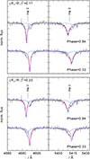 |
Fig. 1. Two example X-shooter spectra (gray) taken close to maximum RV separation. Light gray regions indicate the location of a weak residual nebular line; these have been excluded from the fit. The red and blue lines represent the contribution of Star 1 and Star 2, respectively, and the dashed purple line shows the combined fit. Top panel: Predicted line profiles assuming a surface ratio of 0.17. Bottom panel: Line profiles assuming a surface ratio of 0.23. Applying a consistent approach to all spectra, the resulting derived RV semi-amplitudes of Star 2 are K2 = 143 km/s and K2 = 78 km/s for an assumed surface ratio of 0.17 and 0.23, respectively. |
We conclude that neither the atmospheric parameters nor the RV curves of Star 2 can be determined reliably based on the current spectroscopic observations. Therefore, we adopt the parameters obtained from the light-curve analysis for Star 2. For the strong-lined Star 1, we adopt the spectroscopically determined atmospheric parameters and RV curve. We also point out that Star 1 does not display the Balmer line problem; this can be seen in Fig. A.1, where we show the UVB X-shooter spectrum taken at phase 0.84 compared to our best-fitting Tübingen NLTE Model-Atmosphere Package (TMAP5, Werner et al. 2012) models. The atmospheric parameters of both stars, including their errors, are summarized in Table 2 and the RVs as determined assuming a surface ratio of 0.17 are listed in Table 1.
Orbital and stellar parameters of Pa 13.
3.3. Kiel mass
In Fig. 2 we show the position of the two binary CSs of Pa 13 in a Kiel diagram compared to H-shell burning post-AGB tracks (black lines) from Miller Bertolami (2016) and post-RGB tracks (dashed gray lines) from Hall et al. (2013). Star 1 clearly lies in the post-RGB region. Using the post-RGB evolutionary sequences from Hall et al. (2013) and the griddata (linear) interpolation function in SCIPY (Virtanen et al. 2020), we derived a Kiel mass of 0.41 ± 0.02 M⊙ for Star 1.
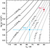 |
Fig. 2. Kiel diagram showing the position of the two CSs of Pa 13 compared to the H-shell burning post-AGB tracks (black lines) from Miller Bertolami (2016) and post-RGB tracks (dashed gray lines) from Hall et al. (2013). |
4. Light- and RV-curve fitting
Simultaneous light- and RV-curve modeling of the CSs of Pa 13 was carried out using PHOEBE2 (Prša et al. 2016; Jones et al. 2020b; Conroy et al. 2020). The spectrum and limb-darkening of both stars were approximated using the same atmosphere models used in Sect. 3.2 as implemented in PHOEBE2 (Jones et al. 2022, 2026), with the effective temperature, surface gravity, and He abundance of Star 1 fixed to the values derived there. For Star 2, we also fixed the He abundance to the value determined previously, but its Teff and logg were allowed to vary freely over a wide range of values.
Given the large relative uncertainty on the Gaia (E)DR3 distance, the fitting was not performed in absolute units, meaning that the fitting accounts for the depths and shapes of the eclipses but not the different brightnesses in the different filters (i.e., only the light-curve morphology not the implied spectral energy distribution). As both stars are clearly hot and compact, extinction will have a minimal impact on the light-curve morphology, nevertheless it was fixed in our modeling to the value determined in Sect. 5.
Via Markov chain Monte Carlo (MCMC) sampling of the model light and RV curves, we derived a best-fitting model. Initially, we fit the RV curves of both stars, and let the radii and masses of both stars, Teff and log g of Star 2, the binary orbital inclination, and the system velocity vary freely. The derived Teff and log g of Star 2 as well as the surface ratio, (R2/R1)2, were then fed back into the spectroscopic analysis.
Upon recognizing the sensitivity of the RV curve of Star 2 to the surface ratio adopted in the spectral fitting (see Sect. 3.2), we revised our modeling strategy. We stress that the surface ratio cannot be independently constrained from the light curves alone, but only the sum of their fractional radii (R1 + R2)/a, where a is the semimajor axis of the binary orbit. Because of this subtle coupling between the surface ratio and the RV curve of Star 2, we consequently fixed the mass, temperature, and surface gravity of Star 1 to the values determined in Sect. 3.2. This includes using the Kiel mass of 0.41 ± 0.02 M⊙ (equivalent to a radius of 0.40 ± 0.04 R⊙) determined by interpolating evolutionary tracks. Similarly, we fit the RV curves derived under the assumption of a surface ratio of (R2/R1)2 = 0.17. This is well justified as the atmospheric parameters and the RV curve of Star 1 showed no significant variation across the individual spectroscopic fits employing different assumed surface ratios, and thus the model mass of Star 2 is principally dependent on the assumed Kiel mass of Star 1 and the inclination (constrained by the light curves).
Our best-fitting model is shown overlaid on the data in Fig. 3, with the parameters listed in Table 2. In this final fit, we derive a binary orbital inclination of  °, and RV semi-amplitudes of K1 = 129 ± 9 km/s and K2 = 136 ± 5 km/s for Star 1 and Star 2, respectively. For Star 2 we find a mass of M2 = 0.39 ± 0.04 M⊙, an effective temperature of
  kK, and a surface gravity of
  (equivalent to a radius of
  ). The resulting surface ratio (0.17) matches the one assumed in the spectroscopic fit (0.17). In addition, the predicted RV curve for Star 2 that is obtained from our final PHOEBE2 model (dashed blue line in the bottom panel of Fig. 3), agrees well with the RV curve determined for Star 2 in the spectroscopic fit assuming (R2/R1)2 = 0.17 (blue crosses in the bottom panel of Fig. 3). Notably, also the system velocity obtained from the RV-curve fitting (vsys = 33.8 ± 6.0 km/s) is in excellent agreement with the systemic velocity inferred from the nebular emission lines in Sect. 3.1 (vsys = 33.7 ± 0.8 km/s). This consistency provides an important sanity check and supports the reliability of the RV curve (see also Reindl et al. 2020).
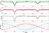 |
Fig. 3. Top three panels: Our best fit eccentric PHOEBE model (black) compared to the observed ZTF g- (green) and r-band (red) and SARA i-band (brown) light curves. The gray line indicates our best model that does not account for eccentricity in the fit. Bottom panel: RVs of Star 1 (red crosses) and Star 2 (blue crosses) as measured assuming a surface ratio of 0.17. The formal fitting error bars for the assumed surface ratio (0.17) are smaller than the symbol sizes. The red and the pink lines indicate the best fit to the RV curve of Star 1 from the eccentric and circular model, respectively. For Star 2 the predicted RV curves from our best fit eccentric and circular model are indicated by the dashed blue and cyan lines, respectively. The gray dashed-dotted line indicates the system velocity. |
Intriguingly, an eccentricity of e = 0.02 is required to fit the light curve; this is highlighted by the fact that the primary and secondary eclipses are not separated by exactly 0.5 in phase. This is particularly apparent in the secondary eclipse (during which Star 1 is obscured) as shown in Fig. 3. The black line represents our best-fitting model, which includes the eccentricity of 0.02, whereas the light-gray curve shows the best-fitting model assuming a circular orbit (note that all parameters other than the eccentricity are within one sigma of the best-fitting model, which allows for eccentricity). The circular model clearly predicts a secondary eclipse that occurs precisely at phase 0.5, appreciably earlier than observed. The impact of the eccentricity on the primary eclipse as well as the RV curves is less obvious. It is important to note that, given the long time coverage of the ZTF light curve and the excellent agreement with the RVs, it is highly unlikely that the implied eccentricity is a phasing issue due to an incorrect orbital period. Rømer delay can also result in eclipses not being separated by 0.5 in phase; however, the clearly similar masses (as implied by the RV curves) imply a negligible delay (Barlow et al. 2012) – certainly not of the order of the observed delay (≈230s or 0.07 in phase). Finally, we note that our best-fitting model does show mild ellipsoidal modulation, just as proposed by Chen et al. (2025).
5. Spectral energy distribution
We performed a two-component fit to the observed spectral energy distribution (SED, see Fig. 4) and employed the χ2 SED fitting routine described in Heber et al. (2018) and Irrgang et al. (2021). We used photometry from Gaia/(E)DR3 (Gaia Collaboration 2021a,b), Skymapper (Onken et al. 2019), and the United Kingdom Infrared Telescope Hemisphere Survey (UHS, Schneider et al. 2025). In the fit we assumed a surface ratio of 0.17, kept the atmospheric parameters fixed, and only let the angular diameter, Θ, and the color excess, E(44 − 55)6, vary freely. Interstellar reddening was accounted for by using the reddening law of Fitzpatrick et al. (2019)7 with RV = 3.1. To compute the Gaia/distance, a Gaussian distributed array of parallaxes was generated, with the distance being the median of this distribution (see Irrgang et al. 2021 for further details). The Gaia parallax was corrected for the zeropoint bias using the Python code provided by Lindegren et al. (2021)8 and the parallax uncertainties are corrected by Eq. (16) in El-Badry et al. (2021).
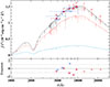 |
Fig. 4. Two-component spectral energy distribution fit. Top panel: Filter-averaged fluxes converted from observed magnitudes are shown in different colors (Gaia: blue, Skymapper: red, UHS: pink). The light red and blue lines correspond to the flux contribution of Star 1 and Star 2, respectively, and the gray line is the combined best fit to the observation. The model fluxes are degraded to a spectral resolution of 6 Å. To reduce the steep SED slope, the flux is multiplied by the wavelength cubed. Bottom panel: Uncertainty-scaled difference between synthetic and observed magnitudes. |
We derive a reddening of EB − V = 0.405 ± 0.005 mag, which is higher than what is suggested by the 2D dust map of Schlafly & Finkbeiner (2011), which predicts EB − V = 0.339 ± 0.011 mag. This indicates that the PN contributes to the reddening of the system.
From the angular diameter and parallax, the radii of the two stars can be calculated via R = Θ/2ϖ. By that we obtain  and
and  , which agree well with the radii obtained from the light-curve fitting.
6. Kinematic analysis
Pa 13 is located at  kpc below the Galactic plane, i.e., in a region where the thick disk dominates (Kordopatis et al. 2011). To further characterize the Galactic population membership of Pa 13, we calculated the space velocities (U points away from the Galactic centre, V points in the direction of Galactic rotation, and W points toward Galactic north). This was done by using the system velocity derived in Sect. 3.1, along with the proper motions and parallaxes from the Gaia (E)DR3. From the Toomre diagram, which is shown in Fig. 5, it becomes clear that Pa 13 exhibits typical halo kinematics.
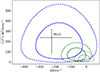 |
Fig. 5. Toomre diagram showing the location of Pa 13. The solid and dashed lines indicate the one- and two-sigma contours, respectively, of the U, V, and W velocity distributions of main-sequence stars from Kordopatis et al. (2011). The gray, green, and blue lines indicate the velocity distribution of thin disk, thick disk, and Galactic halo stars, respectively. |
7. Discussion
7.1. Eccentricity
We reported that Pa 13 shows clear evidence of an eccentric orbit (e = 0.02 ± 0.01). Similar levels of eccentricity have been found in several other post-CE systems containing more evolved WDs or hot subdwarf stars that lack a PN (Kruckow et al. 2021). Among CSPNe, the only other system that shows evidence of eccentricity is NGC 6026. By modeling its light and RV curves, Hillwig et al. (2010) found that the photometric variability is consistent with ellipsoidal modulation, where the CS nearly fills its Roche lobe and the companion is likely a hot WD. The light curves show unequal maxima, which – in the case of ellipsoidal variability – only happens at this amplitude for a noncircular orbit9. Hillwig et al. (2010) showed that the CS light curve in NGC 6026 could be reproduced with an eccentricity in the range e = 0.01 − 0.03.
The eccentricities observed in some post–CE binaries are thought to arise either from the pre-existing eccentricity (Glanz & Perets 2021) or it may have been generated during the CE due to gravitational drag (Szölgyén et al. 2022; Röpke & De Marco 2023). One- and three-dimensional hydrodynamic simulations of CE evolution show that even if the pre-CE binary is initially circular, the resulting post-CE binary may have a nonzero eccentricity of the order of e ≈ 10−2 (Sand et al. 2020; Bronner et al. 2024), i.e., exactly what is observed for Pa 13 and NGC 6026.
Interestingly, the first two eccentric double-WD post-CE binaries have only recently been reported by van Roestel et al. (2025). Those authors find for GALEX J023834.9+093301 and ZTF J175812.85+764216.8 eccentricities of e = (1.55 ± 0.08)×10−3 and e = (1.75 ± 0.15)×10−3, respectively, which are about one order of magnitude lower than what is found for the two eccentric CSPNe. The cooling ages of the two eccentric double WDs are of the order of 108 yr, i.e., roughly four orders of magnitude larger than the post-CE ages of the eccentric CSPNe. The extreme rarity of eccentric double WDs compared to younger, eccentric double-degenerate systems, may therefore reflect the progressive circularization of post-CE binaries over time.
7.2. Formation of the system
Our kinematic analysis has shown that Pa 13 most likely belongs to the Galactic halo. The age of the inner Galactic halo is estimated to be 10.9 ± 0.4 Gyr (Kilic et al. 2019), which then should also correspond to the age of the Pa 13 binary system. With this information, we can exclude that both stars are low-mass (≈0.33 − 0.5 M⊙) CO-core WDs. This is because the initial mass range to produce low-mass CO-core WDs is between approximately 1.8 − 3.0 M⊙ (Prada Moroni & Straniero 2009). The corresponding main-sequence lifetimes of such stars at Z = 0.001 is smaller than one Gyr according to BaSTI evolutionary models10, i.e., about an order of magnitude smaller than the age of the inner Galactic halo.
Furthermore, we can rule out the possibility that the initially more massive star (from now on Star A) evolved first to become a He-core WD and that the other, initially less massive Star B recently turned into a low-mass CO-core pre-WD. Let us assume Star A with initial mass, MA, first evolves into ≈0.4 M⊙ He-core WD. If we further presume that mass transfer was conservative, Star B (with initial mass, MB), would have a post-mass-transfer mass of  . We require
  for the formation of a low-mass CO-core WD, which again implies a main-sequence lifetime of less than one Gyr. In order to match the age of the inner Galactic halo, Star A then would need to have had a main-sequence lifetime of ≈10 Gyr, which would require MA ≈ 0.9 M⊙ according to BaSTI evolutionary models. However, this would then imply Star A was not able to transfer enough mass to obtain
  .
.
Therefore, we conclude that the star that initiated the final CE episode must be a He-core pre-WD. If so, the PN must have been ejected by an RGB star. This provides the strongest evidence so far that the PNe phenomenon is not restricted to AGB stars, but that it can also be witnessed around post-RGB objects (Jones et al. 2023).
Now, let us consider that both CSs of Pa 13 harbor a He-core. He-core WDs evolve from binaries in which both components had an initial mass of ⪅2.3 M⊙ and filled their Roche lobes before helium ignition occurred in its degenerate core. Such systems may either form through “double spiral-in” – also called double-core CE evolution – or following two mass transfer episodes (Nelemans et al. 2001b).
7.2.1. Double-core CE evolution
For double-core CE evolution to occur, the components of the binary must possess almost equal initial masses. The reason for that is that the secondary must have left the main-sequence by the time the primary fills its Roche lobe, while the primary must do so before reaching the tip of the RGB (Brown 1995; Nelemans et al. 2001b; Dewi et al. 2006; Justham et al. 2011). Initially, the system undergoes stable mass transfer, but when the secondary expands due to accretion, it ultimately overfills its Roche lobe. This prompts both stars to enter a CE phase at the same time and the successful ejection of the envelope leaves behind a compact binary consisting of the stripped cores of both components. Although double-core CE evolution is thought to be very rare given the highly constrained parameter space, recent observations have revealed a strong candidate for a progenitor system for this scenario (BD+20 5391, Kurpas et al. 2025).
The mass ratio of Pa 13 is indeed close to unity, which indicates that it may be a viable candidate for the double-core CE evolution scenario. Given the short lifetimes of PNe (≈104 yr), additional confirmation would be valuable for constraining the frequency of double-core evolution. We also note that this may not simply be a fortunate detection as an observational bias is expected among double-lined systems. Detecting double-lined, double-degenerate binaries generally requires both components to have comparable luminosities and post-RGB or post-AGB lifetimes, which in turn implies similar masses.
7.2.2. Two mass transfer episodes with subsequent rejuvenation
The more common case to form a close double He-core WD pair involves two mass transfer episodes. The initially more massive star evolves first, expands to fill its Roche lobe, and transfers mass to its companion. The physics of the first mass transfer episode remains poorly constrained. Nelemans et al. (2025) show that the commonly adopted prescriptions for stable mass transfer and CE evolution in binary population models do not simultaneously reproduce the observed double He-core WD population, which indicates that the treatment of angular-momentum loss during these phases remains uncertain. In this scenario Star A evolves first into a He-core WD and cools until Star B starts to fill its Roche lobe. Mass loss then proceeds on a dynamical timescale that is expected to trigger dynamically unstable mass transfer and the formation of a CE. This results in a drastic shrinkage of the orbit and the formation of a close, double He-core WD pair (Nelemans et al. 2001b).
Note that we cannot completely rule out the possibility of Star A being a low-mass CO WD or hybrid He-CO WD (Zenati et al. 2019) that formed after the first mass transfer episode. This would, however, imply a large difference between the main-sequence lifetimes of both stars (ΔτMS ≈ 10 Gyr) given that they belong to the Galactic halo (see also above). This in turn would imply that Star A then already had enough time to cool down to log L/L⊙ ⪅ −4.0 and Teff ⪅ 6000 K (Prada Moroni & Straniero 2009).
Regardless of whether Star A is a He- or CO-core WD, a central prerequisite for the two mass transfer episodes scenario is that the initially more massive Star A needs to be effectively rejuvenated after the CE ejection, enabling it to evolve once again into a pre–WD configuration and to also stay in this configuration during the PN phase. Such a rejuvenation process of the WD that formed after the first mass transfer episode was also proposed for Hen 2-428, the only other double-lined, double-eclipsing, double-pre-WD system inside a PN. The formation of the system was explained by an initial stable mass transfer episode that resulted in a 0.35 M⊙ He-core WD and a 2.5 M⊙ main-sequence star (Reindl et al. 2020). After about 500 Myr, the latter evolved up the early AGB, a CE was formed, and later ejected. This implies that the He-core WD had enough time to cool down to ≈0.3 L⊙ and Teff ≈ 25 kK (Hall et al. 2013), yet it is also found in a pre-WD configuration with Teff = 40 kK and L = 665 L⊙.
In the case of Pa 13, even if Star B evolved away from the main sequence soon after the first mass transfer event, it would take the red giant between 100 Myr and ≈1 Gyr to form a He core of ≈0.4 M⊙ (Miller Bertolami 2016). During this time the core of Star A would have already cooled and faded down significantly. Consequently, we expect the rejuvenated WD to harbor a much cooler core than those of freshly born post-RGB stars. These rejuvenated objects with cold cores are known to be brighter, and evolve faster, than “normal” post-RGB stars (e.g., Miller Bertolami et al. 2011; Althaus et al. 2013; Istrate et al. 2014). The higher Teff of Star 2 in Pa 13 makes it the most likely candidate for the rejuvenated star in the system (i.e., Star A). If this is the case, then Star 1 in Pa 13 would be the last to evolve (i.e., Star B) and the one with a normal post-RGB core.
7.3. Post-CE evolutionary state and envelope masses
A reliable characterization of the evolutionary status of both stars based solely on their surface parameters (Teff, logg, and log L) is not possible due to the current lack of understanding of the CE event. Thermal equilibrium models such as those computed by Hall et al. (2013) can predict the post-RGB heating and contracting timescales (as well as the corresponding tracks) robustly for stars with a young (hot) He-core11, but the starting point of the post-CE evolution (Teff0, g0, R0) in the Hertzsprung–Russell or Kiel diagram depends on the mass of the H envelope that survives the CE. Current models of the CE event do not provide us with this quantity. It is worth of note that, in the case of Pa 13, the presence of a PN around the system might help us to shed light on the immediate post-CE conditions.
Assuming a distance of 6.9 kpc, a PN diameter of 29 arcsec (as listed in the HASH database), and a typical expansion velocity of 20 km/s (Schönberner et al. 2018), a kinematical age of 24 kyrs can be calculated for the PN. For the typical inferred mass of both stars (≈0.4 M⊙), the 0.403 M⊙ track from Hall et al. (2013) predicts a rather constant heating rate of dTeff/dt ≃ 0.65 K/yr (during the evolution at constant luminosity). This, together with the derived post-CE age from the PN would imply that the effective temperatures of the stars in Pa 13 immediately after the CE (Teff0) have been ≈15.6 kK lower than today. Notably, if this is the case, it would mean that immediately afterwards the CE Star 1 in Pa 13 had a radius of R0 ≃ 0.8 R⊙, which is exactly the size of its Roche lobe at its current separation (a = 2.1 R⊙, q ≃ 1, Eggleton 1983).
Therefore, it is possible to speculate that when the PN was ejected during the CE approximately 24 kyr ago, both stars were still filling their Roche lobes in an over-contact configuration (with Teff0 ≈ 35 kK). The system subsequently became detached as both components contracted, with Star 2 contracting faster due to its possibly rejuvenated nature. Within this picture, detached systems such as Pa 13 would be more evolved analogs of over-contact systems like Hen 2-428.
Interestingly, the derived immediate post-CE effective temperatures, Teff0, can be used to estimate the envelope masses immediately after the CE. This is because, for a given core mass, the starting point of the post-CE evolution in the Kiel or Hertzsprung–Russell diagram (Teff0, g0, R0) of a thermal equilibrium remnant is solely determined by its envelope mass. As envelope masses are not provided by Hall et al. (2013) for their post-RGB models, we computed our own 0.4 M⊙ post-RGB model using the LPCODE code (Miller Bertolami 2016; Miller Bertolami et al. 2022). Our 0.4 M⊙ model reproduces the post-RGB evolution computed by Hall et al. (2013) very closely. These models predict that Star 1 and Star 2 were left with H-rich envelopes of masses  and
and  , respectively, immediately after the CE event12.
It is worthwhile mentioning that these envelopes of masses are well below the critical “peel-off” masses13 for these stars ( for a star departing the RGB at 5000 K, see Hall et al. 2013 for a detailed discussion). This indicates that envelope masses after the CE are very likely smaller than the peel-off mass. Consequently, characterizing double-degenerate CSPNe offers an interesting avenue to constrain the mass ejection process during the CE.
However, these estimations should not be taken at face value for two main reasons. Firstly, within current uncertainties in the mass, heating timescales can vary by a factor of two. For example Hall et al. (2013) predict heating rates of dTeff/dt ≃ 1.2 K/yr and 0.32 K/yr for their 0.427 M⊙ and 0.378 M⊙ post-RGB models, respectively. This will affect the estimation of the immediate post-CE effective temperatures. Moreover, if one of the two CSs is a rejuvenated object, the use of post-RGB models with hot cores will lead to an underestimation of the heating rate. Rejuvenated post-RGB-like structures – such as He-core WDs undergoing a H-shell flash – have a burning shell on top of a more compact He-core. These objects are known to be brighter and harbor thinner H-rich envelopes, which in turn leads to much faster heating rates (e.g., Miller Bertolami et al. 2011; Althaus et al. 2013; Istrate et al. 2014; Althaus et al. 2025).
Regardless of these uncertainties, the previous discussion highlights the fact that young post-CE systems that are still surrounded by a PN might allow us to infer critical information on the CE event itself. In particular, in the case of Pa 13 at least one of the two stars has to be a young post-RGB star (i.e., one that is properly described by the models computed by Hall et al. 2013) that was left after the CE with an envelope mass significantly less massive than the peel-off mass. This result offers a key constraint for hydrodynamical models of the CE ejection.
7.4. Fate of the system
Last but not least, we would like to comment on the fate of the system. Since the eccentricity of the system is small, we calculate the Peters’ timescale, τP (Peters 1964, see also Zwick et al. 2020) to estimate the time the orbit will decay due to the radiation of gravitational waves via
 (2)
(2)
where c is the speed of light, G the gravitational constant, q = M2/M1 ≤ 1 the mass ratio of the system, M the total system mass, a0 the initial Keplerian semimajor axis, and f(e0) the correction of the merger time due to the initial eccentricity of the orbit, e0, which can be calculated via
 (3)
(3)
Using this equation we estimate a merger time of  Gyr. This implies that the system will not merge within a Hubble time, which is also illustrated in Fig. 6.
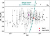 |
Fig. 6. Total mass plotted against logarithmic period of DD systems. Pa 13 is shown in red and Hen 2-428 in purple. The black dots are close double WD systems compiled by Munday et al. (2024). The teal dashed-dotted line indicates which systems will merge within a Hubble time, and the black dashed line indicates the Chandrasekhar mass limit. |
However, when the system eventually merges, a possible outcome is the formation of a highly magnetic (≈200 − 500 kG) He-sdO. Strikingly, all known magnetic He-sdOs have inferred masses of about 0.8 M⊙ (Dorsch et al. 2022, 2024; Pelisoli et al. 2022), which is close to the maximum mass expected from the merger of two He-core WDs and about the total mass of the CSs of Pa 13. About one percent of all He-sdOs exhibit magnetic fields stronger than 100 kG, and it has been suggested that this small fraction may be linked to the requirement that the progenitor He-WDs have coeval masses (Pakmor et al. 2024).
8. Conclusion
In this work we reported that Pa 13 is the second double-eclipsing and double-lined, pre-WD system inside a PN, but the first detached system of this type. Furthermore, we found that Pa 13 provides the strongest evidence so far that the PN phenomenon is not restricted to post-AGB stars, but can also be observed around post-RGB stars. The high quality light curves allowed us to derive an orbital eccentricity of 0.02 ± 0.01, making Pa 13 the second post-CE binary CS with a measured eccentricity.
Since the mass ratio of Pa 13 is close to unity, the system may have formed through double-core CE evolution. Alternatively, the system may have formed following two mass transfer episodes. In the latter case, systems like Pa 13 and Hen 2-428 would indicate that there must exist an efficient CE-induced rejuvenation mechanism capable of reheating the cool WD in the binary, possibly an extreme analog to the observed heating and inflation observed in main-sequence star companions of post-CE CSPNe.
Assuming a kinematical age of 24 kyr, we infer that immediately after the CE ejection the effective temperatures of both components of Pa 13 were ≈15.6 kK lower than today and that Star 1 in Pa 13 must still have filled its Roche lobe. This suggests that Pa 13 represents a more evolved, detached descendant of over-contact double-degenerate systems such as Hen 2-428.
The inferred immediate post-CE effective temperatures, Teff0, also allowed us to place direct constraints on the hydrogen-envelope masses of the two components in Pa 13, since Teff0 of post-RGB models of a given mass is mainly dictated by the residual envelope mass. We estimated post-CE envelope masses that are about a factor of two smaller than the typical peel-off mass for a post-RGB remnant. This demonstrates that double-degenerate systems still embedded within PNe offer particularly powerful constraints on the system’s immediate post-CE configuration (e.g., Teff0, g0, R0) and a direct means of assessing envelope masses. Expanding observational efforts to identify and characterize additional double-degenerate systems inside PNe is thus strongly encouraged.
For Pa 13, higher S/N spectroscopic observations, higher cadence and S/N light curves, and a framework capable of simultaneously fitting spectra, light curves, and RV curves would help to better constrain the system parameters in the future. Follow-up imaging and spectroscopy of the PN are also encouraged to resolve its morphology and to determine its expansion velocity and chemistry. In addition, evolutionary models capable of reproducing the formation of this system would be highly desirable.
Acknowledgments
We thank the Anonymous Referee for their careful review and valuable suggestions. We thank Stephan Geier for helpful discussion. N.R. is supported by the Deutsche Forschungsgemeinschaft (DFG) through grant RE3915/2-1. T.H. acknowledges support from the National Science Foundation: this material is based upon work supported by the National Science Foundation under Award No. AST2107768. Any opinions, findings and conclusions or recommendations expressed in this material are those of the authors and do not necessarily reflect the views of the National Science Foundation. D.J. acknowledges support from the Agencia Estatal de Investigación del Ministerio de Ciencia, Innovación y Universidades (MCIU/AEI) under grant “Nebulosas planetarias como clave para comprender la evolución de estrellas binarias” and the European Regional Development Fund (ERDF) with reference PID-2022-136653NA-I00 (DOI:10.13039/501100011033). DJ also acknowledges support from the Agencia Estatal de Investigación del Ministerio de Ciencia, Innovación y Universidades (MCIU/AEI) under grant “Revolucionando el conocimiento de la evolución de estrellas poco masivas” and the European Union NextGenerationEU/PRTR with reference CNS2023-143910 (DOI:10.13039/501100011033). M3B acknowledges support from CONICET and Agencia I+D+i through grants PIP-2971 and PICT 2020-03316, as well as from the CONICET-DAAD 2022 bilateral cooperation grant number 80726. Based on observations made with the GTC telescope, in the Spanish Observatorio del Roque de los Muchachos of the Instituto de Astrofísica de Canarias, under Director’s Discretionary Time. This paper uses data taken with the MODS spectrographs built with funding from NSF grant AST-9987045 and the NSF Telescope System Instrumentation Program (TSIP), with additional funds from the Ohio Board of Regents and the Ohio State University Office of Research. Based on observations collected at the European Organisation for Astronomical Research in the Southern Hemisphere under ESO programmes 0109.D-0237(A) and 0111.D-2143(A). IRAF is distributed by the National Optical Astronomy Observatory, which is operated by the Association of Universities for Research in Astronomy (AURA) under a cooperative agreement with the National Science Foundation. This work has made use of BaSTI web tools. This research has made use of the HASH PN database at http://hashpn.space. This research made use of the SIMBAD database, operated at CDS, Strasbourg, France; the VizieR catalogue access tool, CDS, Strasbourg, France. This research has made use of the services of the ESO Science Archive Facility. This work has made use of data from the European Space Agency (ESA) mission Gaia (https://www.cosmos.esa.int/gaia), processed by the Gaia Data Processing and Analysis Consortium (DPAC, https://www.cosmos.esa.int/web/gaia/dpac/consortium). Funding for the DPAC has been provided by national institutions, in particular the institutions participating in the Gaia Multilateral Agreement. Based on observations obtained with the Samuel Oschin 48-inch Telescope at the Palomar Observatory as part of the Zwicky Transient Facility project. ZTF is supported by the National Science Foundation under Grant No. AST-1440341 and a collaboration including Caltech, IPAC, the Weizmann Institute for Science, the Oskar Klein Center at Stockholm University, the University of Maryland, the University of Washington, Deutsches Elektronen-Synchrotron and Humboldt University, Los Alamos National Laboratories, the TANGO Consortium of Taiwan, the University of Wisconsin at Milwaukee, and Lawrence Berkeley National Laboratories. Operations are conducted by COO, IPAC, and UW.
References
- Afsar, M., & Ibanoǧlu, C. 2008, MNRAS, 391, 802 [Google Scholar]
- Althaus, L. G., Miller Bertolami, M. M., & Córsico, A. H. 2013, A&A, 557, A19 [NASA ADS] [CrossRef] [EDP Sciences] [Google Scholar]
- Althaus, L. G., Calcaferro, L. M., Córsico, A. H., & Brown, W. R. 2025, A&A, 699, A280 [NASA ADS] [CrossRef] [EDP Sciences] [Google Scholar]
- Antunes Amaral, L., Munday, J., Vučković, M., et al. 2024, A&A, 685, A9 [NASA ADS] [CrossRef] [EDP Sciences] [Google Scholar]
- Barlow, B. N., Wade, R. A., & Liss, S. E. 2012, ApJ, 753, 101 [NASA ADS] [CrossRef] [Google Scholar]
- Bellm, E. C., Kulkarni, S. R., Graham, M. J., et al. 2019, PASP, 131, 018002 [Google Scholar]
- Bhattacharjee, S., Kulkarni, S. R., Kong, A. K. H., et al. 2025, PASP, 137, 024201 [Google Scholar]
- Boffin, H. M. J., Miszalski, B., Rauch, T., et al. 2012, Science, 338, 773 [Google Scholar]
- Bronner, V. A., Schneider, F. R. N., Podsiadlowski, P., & Röpke, F. K. 2024, A&A, 683, A65 [NASA ADS] [CrossRef] [EDP Sciences] [Google Scholar]
- Brown, G. E. 1995, ApJ, 440, 270 [NASA ADS] [CrossRef] [Google Scholar]
- Burdge, K. B., Coughlin, M. W., Fuller, J., et al. 2019, Nature, 571, 528 [Google Scholar]
- Chen, P., Fang, X., Chen, X., & Liu, J. 2025, ApJ, 980, 227 [Google Scholar]
- Chornay, N., & Walton, N. A. 2020, A&A, 638, A103 [NASA ADS] [CrossRef] [EDP Sciences] [Google Scholar]
- Conroy, K. E., Kochoska, A., Hey, D., et al. 2020, ApJS, 250, 34 [Google Scholar]
- Croxall, K. V., & Pogge, R. W. 2019, https://doi.org/10.5281/zenodo.2561424 [Google Scholar]
- Culpan, R., Geier, S., Reindl, N., et al. 2022, A&A, 662, A40 [NASA ADS] [CrossRef] [EDP Sciences] [Google Scholar]
- De Marco, O., Hillwig, T. C., & Smith, A. J. 2008, AJ, 136, 323 [Google Scholar]
- Dewi, J. D. M., Podsiadlowski, P., & Sena, A. 2006, MNRAS, 368, 1742 [NASA ADS] [CrossRef] [Google Scholar]
- Dorsch, M., Reindl, N., Pelisoli, I., et al. 2022, A&A, 658, L9 [NASA ADS] [CrossRef] [EDP Sciences] [Google Scholar]
- Dorsch, M., Jeffery, C. S., Philip Monai, A., et al. 2024, A&A, 691, A165 [NASA ADS] [CrossRef] [EDP Sciences] [Google Scholar]
- Eggleton, P. P. 1983, ApJ, 268, 368 [Google Scholar]
- El-Badry, K., Rix, H.-W., & Heintz, T. M. 2021, MNRAS, 506, 2269 [NASA ADS] [CrossRef] [Google Scholar]
- Evans, C. R., Iben, I., Jr, & Smarr, L. 1987, ApJ, 323, 129 [NASA ADS] [CrossRef] [Google Scholar]
- Filiz, S., Werner, K., Rauch, T., & Reindl, N. 2024, A&A, 691, A290 [NASA ADS] [CrossRef] [EDP Sciences] [Google Scholar]
- Finch, N. L., Braker, I. P., Reindl, N., et al. 2019, ASP Conf. Ser., 519, 231 [NASA ADS] [Google Scholar]
- Fitzpatrick, E. L., Massa, D., Gordon, K. D., Bohlin, R., & Clayton, G. C. 2019, ApJ, 886, 108 [Google Scholar]
- Frew, D. J., Parker, Q. A., & Bojičić, I. S. 2016, MNRAS, 455, 1459 [Google Scholar]
- Gaia Collaboration (Brown, A. G. A., et al.) 2021a, A&A, 649, A1 [NASA ADS] [CrossRef] [EDP Sciences] [Google Scholar]
- Gaia Collaboration (Brown, A. G. A., et al.) 2021b, A&A, 650, C3 [EDP Sciences] [Google Scholar]
- García-Berro, E., Lorén-Aguilar, P., Aznar-Siguán, G., et al. 2012, ApJ, 749, 25 [CrossRef] [Google Scholar]
- García-Segura, G., Ricker, P. M., & Taam, R. E. 2018, ApJ, 860, 19 [CrossRef] [Google Scholar]
- Gentile Fusillo, N. P., Tremblay, P. E., Cukanovaite, E., et al. 2021, MNRAS, 508, 3877 [NASA ADS] [CrossRef] [Google Scholar]
- Glanz, H., & Perets, H. B. 2021, MNRAS, 507, 2659 [NASA ADS] [CrossRef] [Google Scholar]
- Gordon, K. D., Clayton, G. C., Decleir, M., et al. 2023, ApJ, 950, 86 [CrossRef] [Google Scholar]
- Hall, P. D., Tout, C. A., Izzard, R. G., & Keller, D. 2013, MNRAS, 435, 2048 [Google Scholar]
- Heber, U., Irrgang, A., & Schaffenroth, J. 2018, Open Astron., 27, 35 [Google Scholar]
- Higl, J., & Weiss, A. 2017, A&A, 608, A62 [NASA ADS] [CrossRef] [EDP Sciences] [Google Scholar]
- Hillwig, T. C., Bond, H. E., Afşar, M., & De Marco, O. 2010, AJ, 140, 319 [Google Scholar]
- Hillwig, T. C., Bond, H. E., Frew, D. J., Schaub, S. C., & Bodman, E. H. L. 2016a, AJ, 152, 34 [NASA ADS] [CrossRef] [Google Scholar]
- Hillwig, T. C., Jones, D., De Marco, O., et al. 2016b, ApJ, 832, 125 [NASA ADS] [CrossRef] [Google Scholar]
- Hillwig, T. C., Frew, D. J., Reindl, N., et al. 2017, AJ, 153, 24 [Google Scholar]
- Hils, D., Bender, P. L., & Webbink, R. F. 1990, ApJ, 360, 75 [CrossRef] [Google Scholar]
- Irrgang, A., Geier, S., Heber, U., et al. 2021, A&A, 650, A102 [NASA ADS] [CrossRef] [EDP Sciences] [Google Scholar]
- Istrate, A. G., Tauris, T. M., Langer, N., & Antoniadis, J. 2014, A&A, 571, L3 [NASA ADS] [CrossRef] [EDP Sciences] [Google Scholar]
- Jones, D., Boffin, H. M. J., Rodríguez-Gil, P., et al. 2015, A&A, 580, A19 [NASA ADS] [CrossRef] [EDP Sciences] [Google Scholar]
- Jones, D., Boffin, H. M. J., Hibbert, J., et al. 2020a, A&A, 642, A108 [NASA ADS] [CrossRef] [EDP Sciences] [Google Scholar]
- Jones, D., Conroy, K. E., Horvat, M., et al. 2020b, ApJS, 247, 63 [Google Scholar]
- Jones, D., Munday, J., Corradi, R. L. M., et al. 2022, MNRAS, 510, 3102 [CrossRef] [Google Scholar]
- Jones, D., Hillwig, T. C., Reindl, N., et al. 2023, in Highlights on Spanish Astrophysics XI, eds. M. Manteiga, L. Bellot, P. Benavidez, et al., 216 [Google Scholar]
- Jones, D., Corradi, R. L. M., García Pérez, G. A., et al. 2026, A&A, 707, A169 [NASA ADS] [CrossRef] [EDP Sciences] [Google Scholar]
- Justham, S., Podsiadlowski, P., & Han, Z. 2011, MNRAS, 410, 984 [CrossRef] [Google Scholar]
- Kawka, A., Vennes, S., & Ferrario, L. 2020, MNRAS, 491, L40 [Google Scholar]
- Keel, W. C., Oswalt, T., Mack, P., et al. 2017, PASP, 129, 015002 [Google Scholar]
- Kilic, M., Bergeron, P., Dame, K., et al. 2019, MNRAS, 482, 965 [Google Scholar]
- Kordopatis, G., Recio-Blanco, A., de Laverny, P., et al. 2011, A&A, 535, A107 [NASA ADS] [CrossRef] [EDP Sciences] [Google Scholar]
- Kronberger, M., Jacoby, G. H., Acker, A., et al. 2014, in Asymmetrical Planetary Nebulae VI Conference, eds. C. Morisset, G. Delgado-Inglada, & S. Torres-Peimbert, 48 [Google Scholar]
- Kruckow, M. U., Neunteufel, P. G., Di Stefano, R., Gao, Y., & Kobayashi, C. 2021, ApJ, 920, 86 [NASA ADS] [CrossRef] [Google Scholar]
- Kurpas, M., Dorsch, M., Geier, S., et al. 2025, A&A, 702, A200 [NASA ADS] [CrossRef] [EDP Sciences] [Google Scholar]
- Li, Z., Chen, X., Chen, H.-L., et al. 2020, ApJ, 893, 2 [NASA ADS] [CrossRef] [Google Scholar]
- Lindegren, L., Bastian, U., Biermann, M., et al. 2021, A&A, 649, A4 [EDP Sciences] [Google Scholar]
- Lipunov, V. M., Postnov, K. A., & Prokhorov, M. E. 1987, A&A, 176, L1 [NASA ADS] [Google Scholar]
- Mackensen, N., Reindl, N., Werner, K., Dorsch, M., & Tan, S. 2025, A&A, 700, A24 [NASA ADS] [CrossRef] [EDP Sciences] [Google Scholar]
- Masci, F. J., Laher, R. R., Rusholme, B., et al. 2019, PASP, 131, 018003 [Google Scholar]
- Miller Bertolami, M. M. 2016, A&A, 588, A25 [NASA ADS] [CrossRef] [EDP Sciences] [Google Scholar]
- Miller Bertolami, M. M., Althaus, L. G., Olano, C., & Jiménez, N. 2011, MNRAS, 415, 1396 [Google Scholar]
- Miller Bertolami, M. M., Battich, T., Córsico, A. H., Althaus, L. G., & Wachlin, F. C. 2022, MNRAS, 511, L60 [NASA ADS] [CrossRef] [Google Scholar]
- Miszalski, B., Manick, R., Mikołajewska, J., et al. 2018, MNRAS, 473, 2275 [Google Scholar]
- Miszalski, B., Manick, R., Rauch, T., et al. 2019a, PASA, 36, e042 [CrossRef] [Google Scholar]
- Miszalski, B., Manick, R., Van Winckel, H., & Escorza, A. 2019b, PASA, 36, e018 [Google Scholar]
- Miszalski, B., Manick, R., Van Winckel, H., & Mikołajewska, J. 2019c, MNRAS, 487, 1040 [Google Scholar]
- Munday, J., Jones, D., García-Rojas, J., et al. 2020, MNRAS, 498, 6005 [Google Scholar]
- Munday, J., Pelisoli, I., Tremblay, P. E., et al. 2024, MNRAS, 532, 2534 [NASA ADS] [CrossRef] [Google Scholar]
- Napiwotzki, R., Christlieb, N., Drechsel, H., et al. 2001, Astron. Nachr., 322, 411 [NASA ADS] [CrossRef] [Google Scholar]
- Nelemans, G., & Tout, C. A. 2005, MNRAS, 356, 753 [NASA ADS] [CrossRef] [Google Scholar]
- Nelemans, G., Yungelson, L. R., & Portegies Zwart, S. F. 2001a, A&A, 375, 890 [NASA ADS] [CrossRef] [EDP Sciences] [Google Scholar]
- Nelemans, G., Yungelson, L. R., Portegies Zwart, S. F., & Verbunt, F. 2001b, A&A, 365, 491 [NASA ADS] [CrossRef] [EDP Sciences] [Google Scholar]
- Nelemans, G., Preece, H., Temmink, K., Munday, J., & Pols, O. 2025, A&A, 700, A219 [NASA ADS] [CrossRef] [EDP Sciences] [Google Scholar]
- Neunteufel, P., Yoon, S. C., & Langer, N. 2019, A&A, 627, A14 [EDP Sciences] [Google Scholar]
- Onken, C. A., Wolf, C., Bessell, M. S., et al. 2019, PASA, 36, e033 [Google Scholar]
- Pakmor, R., Pelisoli, I., Justham, S., et al. 2024, A&A, 691, A179 [NASA ADS] [CrossRef] [EDP Sciences] [Google Scholar]
- Parsons, S. G., Marsh, T. R., Copperwheat, C. M., et al. 2010, MNRAS, 402, 2591 [Google Scholar]
- Parsons, S. G., Gänsicke, B. T., Marsh, T. R., et al. 2017, MNRAS, 470, 4473 [Google Scholar]
- Pelisoli, I., Dorsch, M., Heber, U., et al. 2022, MNRAS, 515, 2496 [NASA ADS] [CrossRef] [Google Scholar]
- Peters, P. C. 1964, Phys. Rev., 136, 1224 [Google Scholar]
- Pogge, R. 2019, https://doi.org/10.5281/zenodo.2647501 [Google Scholar]
- Pogge, R. W., Atwood, B., Brewer, D. F., et al. 2010, SPIE Conf. Ser., 7735, 77350A [Google Scholar]
- Prada Moroni, P. G., & Straniero, O. 2009, A&A, 507, 1575 [NASA ADS] [CrossRef] [EDP Sciences] [Google Scholar]
- Prochaska, J. X., Hennawi, J. F., Westfall, K. B., et al. 2020, J. Open Source Softw., 5, 2308 [NASA ADS] [CrossRef] [Google Scholar]
- Prša, A., Conroy, K. E., Horvat, M., et al. 2016, ApJS, 227, 29 [Google Scholar]
- Reindl, N., Rauch, T., Werner, K., Kruk, J. W., & Todt, H. 2014, A&A, 566, A116 [NASA ADS] [CrossRef] [EDP Sciences] [Google Scholar]
- Reindl, N., Geier, S., Kupfer, T., et al. 2016, A&A, 587, A101 [NASA ADS] [CrossRef] [EDP Sciences] [Google Scholar]
- Reindl, N., Schaffenroth, V., Miller Bertolami, M. M., et al. 2020, A&A, 638, A93 [NASA ADS] [CrossRef] [EDP Sciences] [Google Scholar]
- Reindl, N., Islami, R., Werner, K., et al. 2023, A&A, 677, A29 [NASA ADS] [CrossRef] [EDP Sciences] [Google Scholar]
- Reindl, N., Bond, H. E., Werner, K., & Zeimann, G. R. 2024, A&A, 690, A366 [NASA ADS] [CrossRef] [EDP Sciences] [Google Scholar]
- Rodríguez-Gil, P., Santander-García, M., Knigge, C., et al. 2010, MNRAS, 407, L21 [NASA ADS] [Google Scholar]
- Röpke, F. K., & De Marco, O. 2023, Liv. Rev. Comput. Astrophys., 9, 2 [CrossRef] [Google Scholar]
- Sand, C., Ohlmann, S. T., Schneider, F. R. N., Pakmor, R., & Röpke, F. K. 2020, A&A, 644, A60 [NASA ADS] [CrossRef] [EDP Sciences] [Google Scholar]
- Santander-García, M., Rodríguez-Gil, P., Corradi, R. L. M., et al. 2015, Nature, 519, 63 [Google Scholar]
- Schlafly, E. F., & Finkbeiner, D. P. 2011, ApJ, 737, 103 [Google Scholar]
- Schneider, A. C., Vrba, F. J., Bruursema, J., et al. 2025, AJ, 170, 86 [Google Scholar]
- Schönberner, D., & Steffen, M. 2019, A&A, 625, A137 [NASA ADS] [CrossRef] [EDP Sciences] [Google Scholar]
- Schönberner, D., Balick, B., & Jacob, R. 2018, A&A, 609, A126 [NASA ADS] [CrossRef] [EDP Sciences] [Google Scholar]
- Shen, K. J. 2025, ApJ, 982, 6 [Google Scholar]
- Szölgyén, Á., MacLeod, M., & Loeb, A. 2022, MNRAS, 513, 5465 [CrossRef] [Google Scholar]
- van Roestel, J., Burdge, K., Caiazzo, I., et al. 2025, A&A, accepted [arXiv:2505.15580] [Google Scholar]
- Vernet, J., Dekker, H., D’Odorico, S., et al. 2011, A&A, 536, A105 [NASA ADS] [CrossRef] [EDP Sciences] [Google Scholar]
- Virtanen, P., Gommers, R., Oliphant, T. E., et al. 2020, Nat. Methods, 17, 261 [Google Scholar]
- Webbink, R. F. 1984, ApJ, 277, 355 [NASA ADS] [CrossRef] [Google Scholar]
- Werner, K. 1996, ApJ, 457, L39 [Google Scholar]
- Werner, K., & Rauch, T. 2015, A&A, 584, A19 [NASA ADS] [CrossRef] [EDP Sciences] [Google Scholar]
- Werner, K., Dreizler, S., & Rauch, T. 2012, Astrophysics Source Code Library [record ascl:1212.015] [Google Scholar]
- Werner, K., Rauch, T., & Kruk, J. W. 2018, A&A, 616, A73 [NASA ADS] [CrossRef] [EDP Sciences] [Google Scholar]
- Wu, C., Xiong, H., & Wang, X. 2022, MNRAS, 512, 2972 [NASA ADS] [CrossRef] [Google Scholar]
- Zenati, Y., Toonen, S., & Perets, H. B. 2019, MNRAS, 482, 1135 [NASA ADS] [CrossRef] [Google Scholar]
- Zhang, X., & Jeffery, C. S. 2012a, MNRAS, 426, L81 [NASA ADS] [CrossRef] [Google Scholar]
- Zhang, X., & Jeffery, C. S. 2012b, MNRAS, 419, 452 [NASA ADS] [CrossRef] [Google Scholar]
- Zwick, L., Capelo, P. R., Bortolas, E., Mayer, L., & Amaro-Seoane, P. 2020, MNRAS, 495, 2321 [Google Scholar]
The gravity mass is defined as  , where gspec is the surface gravity derived from spectroscopy, RGaia the stellar radius obtained by spectral energy distribution fitting assuming the distance from the Gaia mission, and G is the gravitational constant.
Fitzpatrick et al. (2019) employed E(44 − 55), which is the monochromatic equivalent of the usual E(B − V), using the wavelengths 4400 Å and 5500 Å, respectively. For high effective temperatures, such as the nucleus of Pa 13, E(44 − 55) is identical to E(B − V).
We note that more recent reddening curves are available in Gordon et al. (2023).
Similarly appearing unequal maxima can occur in the case of Doppler boosting, but at amplitudes about ten times smaller than observed in NGC 6026.
By robustly we mean specifically that, as long as the object is in the so-called “thermal equilibrium”, and as long as the core has not cooled down from its RGB temperature, both the tracks and the heating rates will not deviate from those computed by Hall et al. (2013).
These masses are very likely underestimated since the post-RGB models were calculated for Z = 0.02 enabling a direct comparison with the models shared by P. D. Halls. At lower metallicity (which is expected for Pa 13), larger envelope masses are to be expected, yet they will still be significantly smaller than the corresponding peel-off mass.
The peel-off mass is defined as the maximum mass of a contracting thermal equilibrium remnant. A thermal equilibrium remnant with a mass greater than this is a red giant and expands as its core mass grows (Hall et al. 2013).
Appendix A: Figure
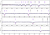 |
Fig. A.1. UVB X-shooter spectrum taken at phase 0.84 (gray) compared to our best-fitting TMAP models assuming a surface ratio of 0.17. Light gray regions indicate the location of a weak residual nebular and interstellar lines, which have been excluded from the fit. The red and blue lines represent the contribution of Star 1 and Star 2, respectively, and the dashed, purple line shows the combined fit. |
All Tables
All Figures
|
Fig. 1. Two example X-shooter spectra (gray) taken close to maximum RV separation. Light gray regions indicate the location of a weak residual nebular line; these have been excluded from the fit. The red and blue lines represent the contribution of Star 1 and Star 2, respectively, and the dashed purple line shows the combined fit. Top panel: Predicted line profiles assuming a surface ratio of 0.17. Bottom panel: Line profiles assuming a surface ratio of 0.23. Applying a consistent approach to all spectra, the resulting derived RV semi-amplitudes of Star 2 are K2 = 143 km/s and K2 = 78 km/s for an assumed surface ratio of 0.17 and 0.23, respectively. |
| In the text | |
|
Fig. 2. Kiel diagram showing the position of the two CSs of Pa 13 compared to the H-shell burning post-AGB tracks (black lines) from Miller Bertolami (2016) and post-RGB tracks (dashed gray lines) from Hall et al. (2013). |
| In the text | |
|
Fig. 3. Top three panels: Our best fit eccentric PHOEBE model (black) compared to the observed ZTF g- (green) and r-band (red) and SARA i-band (brown) light curves. The gray line indicates our best model that does not account for eccentricity in the fit. Bottom panel: RVs of Star 1 (red crosses) and Star 2 (blue crosses) as measured assuming a surface ratio of 0.17. The formal fitting error bars for the assumed surface ratio (0.17) are smaller than the symbol sizes. The red and the pink lines indicate the best fit to the RV curve of Star 1 from the eccentric and circular model, respectively. For Star 2 the predicted RV curves from our best fit eccentric and circular model are indicated by the dashed blue and cyan lines, respectively. The gray dashed-dotted line indicates the system velocity. |
| In the text | |
|
Fig. 4. Two-component spectral energy distribution fit. Top panel: Filter-averaged fluxes converted from observed magnitudes are shown in different colors (Gaia: blue, Skymapper: red, UHS: pink). The light red and blue lines correspond to the flux contribution of Star 1 and Star 2, respectively, and the gray line is the combined best fit to the observation. The model fluxes are degraded to a spectral resolution of 6 Å. To reduce the steep SED slope, the flux is multiplied by the wavelength cubed. Bottom panel: Uncertainty-scaled difference between synthetic and observed magnitudes. |
| In the text | |
|
Fig. 5. Toomre diagram showing the location of Pa 13. The solid and dashed lines indicate the one- and two-sigma contours, respectively, of the U, V, and W velocity distributions of main-sequence stars from Kordopatis et al. (2011). The gray, green, and blue lines indicate the velocity distribution of thin disk, thick disk, and Galactic halo stars, respectively. |
| In the text | |
|
Fig. 6. Total mass plotted against logarithmic period of DD systems. Pa 13 is shown in red and Hen 2-428 in purple. The black dots are close double WD systems compiled by Munday et al. (2024). The teal dashed-dotted line indicates which systems will merge within a Hubble time, and the black dashed line indicates the Chandrasekhar mass limit. |
| In the text | |
|
Fig. A.1. UVB X-shooter spectrum taken at phase 0.84 (gray) compared to our best-fitting TMAP models assuming a surface ratio of 0.17. Light gray regions indicate the location of a weak residual nebular and interstellar lines, which have been excluded from the fit. The red and blue lines represent the contribution of Star 1 and Star 2, respectively, and the dashed, purple line shows the combined fit. |
| In the text | |
Current usage metrics show cumulative count of Article Views (full-text article views including HTML views, PDF and ePub downloads, according to the available data) and Abstracts Views on Vision4Press platform.
Data correspond to usage on the plateform after 2015. The current usage metrics is available 48-96 hours after online publication and is updated daily on week days.
Initial download of the metrics may take a while.