| Issue |
A&A
Volume 709, May 2026
|
|
|---|---|---|
| Article Number | A122 | |
| Number of page(s) | 10 | |
| Section | Astronomical instrumentation | |
| DOI | https://doi.org/10.1051/0004-6361/202555748 | |
| Published online | 07 May 2026 | |
Applying vision transformers to the spectral analysis of astronomical objects
1
Harvard Extension School, Harvard University,
Cambridge,
MA
02138,
USA
2
John A. Paulson School of Engineering and Applied Science, Harvard University,
Cambridge,
MA
02138,
USA
3
Department of Computer Science, Universidad de Concepción,
Edmundo Larenas 219,
Concepción,
Chile
4
Center for Data and Artificial Intelligence, Universidad de Concepción,
Edmundo Larenas 310,
Concepción,
Chile
5
Millennium Institute of Astrophysics (MAS),
Nuncio Monseñor Sotero Sanz 100, Of. 104, Providencia,
Santiago,
Chile
6
Millennium Nucleus for Galaxies (MINGAL),
Chile
7
Heidelberg Institute for Theoretical Studies, Heidelberg,
Baden-Württemberg,
Germany
★ Corresponding author: This email address is being protected from spambots. You need JavaScript enabled to view it.
Received:
30
May
2025
Accepted:
1
March
2026
Abstract
We applied pretrained vision transformers (ViTs), originally developed for image recognition, to the analysis of astronomical spectral data. By converting traditional 1D spectra into 2D image representations, we enable ViTs to capture both local and global spectral features through spatial self-attention. We fine-tuned a ViT pretrained on ImageNet using millions of spectra from the Sloan Digital Sky Survey (SDSS; Kollmeier et al. 2019, in BAAS, 51, 274; Stoughton et al. 2002, AJ, 123, 485) and Large Sky Area Multi-Object Fiber Spectroscopic Telescope (LAMOST; Luo et al. 2015, Res. Astron. Astrophys., 15, 1095) surveys, represented as spectral plots. Our model is evaluated on key tasks including stellar object classification and redshift (z) estimation, where it demonstrates strong performance and scalability. We achieved classification accuracy higher than that of support vector machines and random forests, and we attain R2 values comparable to AstroCLIP’s spectrum encoder, even when generalizing across diverse object types. These results demonstrate the effectiveness of using pretrained vision models for spectroscopic data analysis. To our knowledge, this is the first application of ViTs to large-scale astronomical datasets, which also leverages real spectroscopic data and does not rely on synthetic inputs.
Key words: methods: data analysis / methods: statistical / techniques: miscellaneous / techniques: spectroscopic
© The Authors 2026
 Open Access article, published by EDP Sciences, under the terms of the Creative Commons Attribution License (https://creativecommons.org/licenses/by/4.0), which permits unrestricted use, distribution, and reproduction in any medium, provided the original work is properly cited.
This article is published in open access under the Subscribe to Open model. This email address is being protected from spambots. You need JavaScript enabled to view it. to support open access publication.
1 Introduction
Spectroscopy is a core observational technique in astrophysics for determining the physical and chemical properties of celestial objects, including radial velocities (e.g., for exoplanet detection), stellar oscillations (astroseismology), and the identification of chemically peculiar stars (Burrows & Orton 2010; Fischer & Valenti 2005; Chaplin & Miglio 2013; Preston 1974). By dispersing light into a spectrum, astronomers can extract information about an object’s composition, temperature, radial motion, and even aspects of its structure or environment (Gray 2005). Unlike direct imaging, which mainly provides spatial information, spectroscopic observations probe the underlying physical processes and conditions in astronomical objects such as stars, nebulae, and galaxies. Through spectral analysis, scientists can identify the elements present in them and discern how they exist or interact under extreme cosmic conditions that cannot be replicated in laboratories (Wahlgren 2011).
Spectral data are also essential for understanding the large-scale structure and evolution of the Universe. The redshift of spectral lines provides a key method for measuring cosmic expansion, allowing us to estimate distances to galaxies and trace the large-scale structure of the cosmos (Hubble 1929; Colless et al. 2001). However, galaxy evolution is not solely dictated by their positions and motions in an expanding Universe; their internal chemical composition also shapes it. Spectroscopy plays a crucial role in this aspect, revealing how elements are synthesized in stars, expelled into the interstellar medium, and recycled into subsequent generations of stars (Maiolino & Mannucci 2019). By studying absorption and emission lines, astronomers can track the abundance of elements essential for planetary formation and, ultimately, for the emergence of life (Wolfe et al. 2005).
Modern spectroscopic surveys such as the Sloan Digital Sky Survey (SDSS; Kollmeier et al. 2019; Stoughton et al. 2002) and the Large Sky Area Multi-Object Fiber Spectroscopic Telescope (LAMOST; Luo et al. 2015) have enabled access to datasets containing millions of spectra across diverse object types. These surveys are also making continuous data releases to the public, enabling ground-breaking research to take place. The volume of spectral data continues to grow, with surveys such as Maunakea Spectroscopic Explorer (MSE; Sheinis et al. 2023), 4-metre Multi-Object Spectroscopic Telescope (4MOST; de Jong et al. 2016), the Gaia Mission (Gaia Collaboration 2016), and the Dark Energy Spectroscopic Instrument (DESI; Hahn et al. 2023) now operational or in preparation.
Spectral redshift estimation and classification in surveys such as SDSS typically rely on template-fitting, where observed spectra are matched to composite templates derived from empirically defined object classes (Kügler et al. 2015). These templates are applied to each observed spectrum, allowing predefined properties such as the redshift to be computed by identifying the best fit. However, this approach simplifies the complexity of the data, limiting the precision of individual property estimates (Mészáros et al. 2013; Ness et al. 2015). Furthermore, the reliability of the results is sensitive to the selection and construction of the reference templates. While such automated pipelines improve efficiency over manual inspection, they still operate under constrained assumptions and leave room for more flexible, data-driven approaches that could capture finer-grained spectral features.
Manual inspection introduces uncertainty in redshift determination, which Yang et al. (2018) estimated as σz/(1 + z) < 0.001. One possible cause of this uncertainty is that up to 25% of the input targets in their analysis could be categorized as unreliable due to low S/Ns or ambiguous spectral features. So, even introducing manual inspection leaves possibilities for errors, and, with the size of the surveys, adding extra automated steps to help validate and cross-check means greater reliability with regard to the results.
Machine-learning models offer a promising alternative by learning generalizable spectral representations from datasets. Unlike manual inspection or traditional template-based approaches, these models can capture complex patterns in spectral data and generalize across different observational conditions. Vision transformers (ViTs; Dosovitskiy et al. 2021), a specific deep-learning architecture introduced for image recognition, are particularly promising for spectral analysis due to their ability to capture contextual information in a scalable manner that is also adaptable to multiple downstream tasks, making them suitable for a broad range of astrophysical experiments. Figure 1 shows the architecture of a ViT model.
Vision transformers are derived from transformer architectures, originally developed for natural language processing (Vaswani et al. 2017), which leverage self-attention mechanisms to efficiently model long-range dependencies. Unlike recurrent architectures (Hochreiter & Schmidhuber 1997; Cho et al. 2014) that process sequences sequentially, transformers simultaneously compute relationships between all tokens in parallel, enabling more efficient training and better scalability to long sequences and large datasets. The self-attention mechanism allows each token to assess the relevance of all other tokens, facilitating a contextual understanding that is particularly powerful in language tasks. Transformer architectures adapted for classification tasks, such as BERT (Devlin et al. 2019) and ViT (Dosovitskiy et al. 2021), typically include a special classification (CLS) token that serves as a condensed representation of the entire sequence for downstream prediction tasks. While not present in the original transformer architecture (Vaswani et al. 2017), this CLS token has become a standard component in vision and language models adapted for classification and regression. More recently, transformer-based models have been investigated for spectral data analysis, where self-attention is applied directly to 1D spectral sequences (Koblischke & Bovy 2024; Różański et al. 2025; Pattnaik et al. 2025; Campbell et al. 2026).
When adapted for images, ViTs divide the input image into fixed-sized patches, which are then linearly embedded and combined with positional encodings to preserve spatial structure. These patch embeddings pass through transformer layers, where self-attention captures global interactions across the entire image. Unlike convolutional neural networks (CNNs), a machine-learning approach commonly used for image processing that analyzes images by examining small local regions and gradually combining them into larger patterns (LeCun et al. 1998; Krizhevsky et al. 2012), ViTs inherently model global relationships across the entire image from the earliest layers. This capability motivated our approach to transforming astronomical spectra into 2D image-like representations, enabling effective analysis using ViTs.
Vision transformers typically require very large training and fine-tuning datasets, a requirement that modern astronomy can meet with upcoming massive surveys. We employed state-of-the-art ViTs that were pretrained on regular images from ImageNet (Deng et al. 2009) and fine-tuned it on plots of spectra generated from a combined dataset comprising large portions of SDSS and LAMOST surveys.
We evaluated these models on multiple tasks, including redshift regression, stellar parameter inference, and morphological classification. In both types of tasks (classification and regression), the model shows high accuracy and performs well across a range of S/Ns. Furthermore, this design allows for easy integration of more data sources, such as different surveys, and refinements to the downstream tasks being performed. These results highlight the extensibility and the potential to support a broad range of future applications with our approach.
This paper is organized as follows. Section 2 reviews related work. Section 3 describes the datasets used and their processing. Section 4 outlines the downstream tasks in detail. Section 5 discusses the model architecture. Section 6 presents results, which we discuss in Sect. 7. Finally, Sect. 8 concludes with future steps.
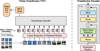 |
Fig. 1 Vision transformer architecture. An input image is divided into fixed-sized patches, which are linearly embedded and combined with positional encodings before being processed through transformer encoder layers. Figure sourced from Dosovitskiy et al. (2021). |
2 Previous work
Several traditional and automated approaches have been developed for redshift estimation using spectroscopic data. Among the most prominent is Redrock (Ross et al. 2020), which is widely used in both the DESI project and recent SDSS data releases. Another notable method is Darth Fader (DF; Machado et al. 2013). Both techniques operate by cross-correlating observed spectra with templates over a range of redshift values and minimizing the χ2 error. These methods do not require prior knowledge of the physical properties of the sources and have demonstrated reasonable performance even under low-S/N conditions.
In the last decade, efforts have incorporated machine-learning techniques to improve redshift regression. Frontera-Pons et al. (2019) introduced two models: one based on dictionary learning (DL) and another on a denoising autoencoder (DAE). The DL model learns a sparse dictionary of galaxy spectra and estimates redshift by minimizing the reconstruction error for a new input spectrum. The DAE model, on the other hand, is trained on synthetic galaxy spectra at zero redshift and estimates redshift by finding the transformation that best reconstructs the observed spectrum. A hybrid model that dynamically selects between DL and DAE based on input characteristics outperforms DF in comparable scenarios. Both Machado et al. (2013) and Frontera-Pons et al. (2019) focused exclusively on galaxies and relied on simulated spectra.
More recently, Podsztavek et al. (2022) proposed a redshift estimation framework using Bayesian CNNs specifically designed to identify potentially unreliable redshift values in large spectroscopic surveys. Their architecture is based on the VGG network (Simonyan & Zisserman 2015) and was trained on real spectroscopic data from Pâris, Isabelle et al. (2017), SDSS Quasar Catalog DR12). To evaluate performance, they also implemented a simpler Bayesian fully connected neural network (Bayesian FCNN) as a baseline. Their implementation treats the input spectrum as a 1D signal, mapping each wavelength to a single flux value, and does not leverage multiple color channels, which are commonly used in standard image processing.
Beyond redshift estimation, other studies have focused on classification tasks using spectroscopic data. In this case, most studies apply dimensionality-reduction techniques, such as the principal component analysis (PCA), followed by clustering or classification algorithms. For instance, Marchetti et al. (2012) used the PCA via Karhunen–Loève projections on galaxy spectra from the VIPERS survey (Scodeggio et al. 2018). After reducing the dimensionality, they applied k-means clustering to group galaxies into early, intermediate, late, and starburst categories. Their method achieved results comparable to photometric approaches while leveraging the richer information content of spectra. However, it exhibited limitations, particularly in underrepresented classes such as active galactic nuclei (AGNs).
Parker et al. (2024) introduced AstroCLIP, a cross-modal foundation model that jointly embeds galaxy images and spectra into a shared latent space through self-supervised transformer encoders aligned via contrastive learning. Their approach uses a ViT-based image encoder and a GPT-2-inspired (Radford et al. 2019) spectral encoder adapted for masked modeling, where spectra are segmented and partially masked to encourage the model to capture meaningful spectral features without labeled data. AstroCLIP, trained on DESI data (Hahn et al. 2023) and Legacy Imaging Survey (DESI-LS; Schlegel et al. 2021) imagery, outperforms supervised baselines on tasks such as stellar mass and metallicity estimation, and significantly improves photometric redshift predictions compared to prior self-supervised methods. Notably, aligning images and spectra helps the spectral embeddings organize more clearly around astrophysical properties, showing how multimodal contrastive learning can outperform traditional single-modality methods.
Although our focus is on spectroscopy, several recent works in photometric classification are relevant for their methodological contributions. At a coarse level of granularity, Wang et al. (2022) carried out a classification of stars, galaxies, and quasi-stellar objects (QSOs) within the J-PLUS survey (Cenarro et al. 2019) using photometric data, finding that support vector machines (SVMs; Cortes & Vapnik 1995) and random forests (RFs; Breiman 2001) achieved nearly equivalent performance. Similar results were reported by Vavilova et al. (2021), which found SVMs and RFs to yield 96.4% and 95.5% accuracy, respectively, while Daoutis et al. (2025) applied RFs to classify galaxies into star-forming, AGN, and passive categories, achieving around 99% overall accuracy with particularly strong performance on star-forming galaxies and slightly lower accuracy for AGNs.
Transformer-based architectures have also been explored in photometric contexts. Donoso-Oliva et al. (2023) introduced a transformer model inspired by BERT (Devlin et al. 2019) for analyzing light curves, which they fine-tuned for both classification and regression tasks. Meanwhile, Cao et al. (2024) combined CNNs with ViTs in a hybrid convolutional visual transformer (CvT) architecture for galaxy morphology classification using image data from Galaxy Zoo (Willett et al. 2013).
While these photometric studies do not operate on spectroscopic inputs, they highlight a broader interest in applying modern architectures, including transformers and ViTs, to astronomical data. Both photometric and spectroscopic observations share similarities as sequential data with comparable observational challenges (e.g., S/N variations and instrumental effects). However, they differ fundamentally in their information content: photometric time series capture temporal evolution, whereas spectra encode wavelength-dependent information with significant long-range dependencies, such as multiple emission or absorption lines arising from the same element at different wavelengths. The self-attention mechanism in transformers may therefore be particularly well-suited for spectroscopic data, as it can naturally capture these long-range spectral correlations that are critical for tasks such as redshift estimation and chemical abundance determination. This motivates our adaptation of ViTs for spectral analysis.
3 Data sources
The training relies on spectroscopic data from two large-scale sky surveys: SDSS, specifically Data Release 181 and LAMOST, with Version 2.0 of Data Release 102. The diversity and volume of spectra from both surveys make them an ideal foundation for training a model capable of learning complex patterns and generalizing across varying observational conditions. In the following subsections, we describe each dataset’s characteristics, including their spectral coverage and selection criteria. For experimentation purposes, we split these datasets into the following categories: medium-sized datasets, which contain a balanced representation across classes; and big datasets, which contain all of the objects in each survey. The medium datasets allowed us to evaluate model performance under controlled conditions where class imbalance does not confound results, while the big datasets test the model’s ability to handle realistic survey data with natural class distributions and assess scalability to large volumes of spectra. Table 1 summarizes the number of objects per morphological class for each dataset and includes a new joint dataset combining SDSS and LAMOST (SLOMOST), which served as the primary dataset for our experiments.
The wavelengths collected from the surveys span from about 3600 to 10 400 Å. The spectra obtained from SDSS have R between 1560 and 2650; therefore, we matched them using the low-resolution subset of the LAMOST survey, which has R ~ 1800.
Figures 2 and 3 show the distribution of redshifts in both datasets across each of the major classes. Figure 4 displays the distribution of S/N values, using the snMedian field provided by SDSS for each object3. Since LAMOST does not provide a precalculated snMedian value, we computed it based on SDSS conventions4.
Dataset sizes in thousands and per-class representation.
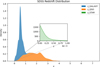 |
Fig. 2 Distribution of redshifts for the SDSS dataset. |
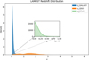 |
Fig. 3 Distribution of redshifts for the LAMOST dataset. |
3.1 SDSS
Operating since 2000, SDSS has mapped millions of celestial objects – including stars, galaxies, and quasars – using fiber-optic spectrographs to capture optical and near-infrared data across a significant portion of the sky. It encompasses multiple spectroscopic programs targeting different object types. Notably, the Baryon Oscillation Spectroscopic Survey (BOSS; Dawson et al. 2013) and Extended BOSS (eBOSS; Dawson et al. 2016) components targeted galaxies up to z ~ 1 and quasars up to z ~ 6.
We excluded objects with zWarning ≠ 0, or with instrument ≠ “BOSS” or targetType ≠ “SCIENCE” From an initial set of 5112k objects, this selection left us with approximately 2767k objects.
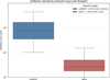 |
Fig. 4 Comparison of snMedian distributions across both datasets via a log-scale box plot. The central box spans the interquartile range (25th–75th percentiles), whiskers extend to the 5th and 95th percentiles, and outliers beyond this range are omitted for clarity. |
3.2 LAMOST
Active since 2012, LAMOST employs a wide-field design and fiber-optic technology to observe up to 4000 objects simultaneously, focusing on stellar kinematics, chemical abundances, and radial velocities. It is optimized for high-throughput spectroscopic surveys of stars in the Milky Way, enabling large-scale studies of the structure, formation history, and kinematics of the Galaxy’s disk and halo.
LAMOST primarily targets objects at z ≈ 0 (Milky Way stars), with only a small fraction of low-redshift extragalactic sources.
We excluded entries where any of the fields z, z_err, snru, snrg, snrr, snri, or snrz were set to −9999, indicating data quality issues. From an initial set of 11 441k objects, this left us with 11 307 objects.
4 Downstream tasks
4.1 Stellar object classification
The first downstream task we consider is the classification of astronomical sources. Traditionally, objects observed in spectroscopic surveys are broadly categorized as stars, galaxies, and quasars. These categories are central to astrophysical studies, enabling insights into stellar evolution, galactic structure, and accretion processes around supermassive black holes. We currently only implement and evaluate classification into broad categories, and though nothing in the model prevents finer sub-divisions, these are left for future studies. These could provide astrophysical insights; for example, stellar spectral types reveal temperature and composition, while galaxy subclasses indicate star formation rates or metallicity. Quasars may be further sub-divided by emission-line characteristics or luminosity classes, and galaxies can be categorized into morphological or spectroscopic subclasses that inform us about their star formation rates, dust content, and metallicity gradients. Classification results are shown in Sect. 6.1, with a comparison of the different plot types in Table 2.
4.2 Redshift regression
The second key downstream task is the estimation of redshift for extragalactic objects. The ViT-based architecture inherently captures global spectral patterns, making it well-suited to detect shifts in characteristic emission and absorption lines without being confounded by local noise or incomplete line profiles. By encoding an entire spectrum as a sequence of contextualized patches, the model can discern small wavelength shifts, even in the presence of multiple lines or low S/Ns. As a result, the model produces accurate redshift estimates, as seen in Table 4 in Sect. 6.2.
4.3 Stellar parameter regression
Beyond redshift estimation, we also experimented with the regression of fundamental stellar parameters, including effective temperature (Teff), surface gravity (log g), and metallicity ([Fe/H]). The ability to infer these values directly from spectra allows for large-scale stellar population studies, aiding in Galactic archaeology and the study of stellar formation histories such as in Gaia (Creevey et al. 2023) and the Apache Point Observatory Galactic Evolution Experiment (APOGEE; Majewski et al. 2017). The results for each individual parameter can be found in Sect. 6.3.
5 Model architecture
We represent the spectral data visually by converting 1D spectra into 2D images. While a 1D architecture might seem more intuitive for inherently 1D spectral data, we adopted this 2D approach for several reasons. First, it enabled us to leverage ViTs pretrained on millions of natural images (Dosovitskiy et al. 2021; Caron et al. 2021), benefiting from transfer learning without requiring expensive pretraining on astronomical data from scratch. Second, 2D representations allow for richer encoding strategies, such as mapping different spectral segments to color channels or spatial arrangements that emphasize specific features. Third, ViTs have demonstrated remarkable success on image data, and recent work in astronomy has shown that visual representations can effectively capture complex patterns in observational data (Parker et al. 2024). Finally, converting spectra to images makes our approach more flexible for future extensions, such as incorporating additional metadata or multimodal inputs. Based on the hypothesis that image-based formats may reveal patterns more readily learnable by pretrained vision models, we explore multiple 2D visualization strategies in the following sections. We also provide a simple 1D transformer implementation that performs redshift regression as a baseline; results for it are given in Sect. 6.2. This simple 1D transformer combines linear projections of flux values and wavelength positions with sinusoidal positional encoding, processes the sequence through multilayer multi-head self-attention (6 layers, 8 heads, 512-dimensional), applies layer normalization and global average pooling over the attended sequence, and outputs predictions through a multi-layer perceptron regression head.
Figure 5 shows an example of a galaxy spectrum that was used as input to the model during experiments. Although it is a direct plot of the spectral values, experiments with this representation already delivered good performance, and for the regression of effective temperature and surface gravity of stars, it proved to be the most effective. We also explored other representations, which either modified the format of how the information was embedded into the final input or attempted to add extra information. In the following sections, we discuss the various processing methods that led to improved performance on each specific task. For consistency and ease of comparison, all subsequent visualizations are based on the same galaxy.
Our underlying model is based on DINO from Caron et al. (2021), a self-supervised learning approach described as a form of self-distillation without labels. The model was pretrained on the ImageNet dataset in an unsupervised manner. We used the pretrained version of DINO as a backbone for our models without pretraining it for spectral data.
For the redshift regression task, we fine-tuned a pretrained ViT model obtained from Hugging Face (namely facebook/dinovitb16), which processes input images resized to 224 × 224 pixels, with a custom regression head. This head consists of a single linear layer that maps the CLS token output from the ViT to a single continuous value representing the predicted redshift. During training, we used the mean squared error (MSE) as the loss function. The input images were normalized using a mean and standard deviation of 0.5 for each color channel.
Figure 6 shows the implemented pipeline, a structured workflow that converts raw spectroscopic data into formats optimized for analysis with ViTs. We now outline each stage of the pipeline, from data acquisition through preprocessing to model pretraining and fine-tuning.
The pipeline begins by acquiring spectroscopic data and metadata from publicly available surveys such as SDSS and LAMOST. These datasets, typically in FITS format, are processed using the AstroPy library (Astropy Collaboration 2022). Each object is then saved as an individual CSV file containing wavelength and flux columns, simplifying downstream processing and model input preparation. Next, several preprocessing steps are applied to ensure data quality and consistency: both the wavelengths and flux values are normalized using minmax scaling, to standardize their representation across different observations and to mitigate variations due to differences in instrument sensitivity or observational conditions, and we performed some control of outlier values by setting up thresholds based on the first and last quartile of the wavelengths from the dataset.
To adapt spectral data for consumption by ViTs, 1D spectra were transformed into 2D image representations. This transformation is a key component of our model design, as the choice of how the spectra are encoded into images can significantly influence performance. Initial experiments used a plot we refer to as “simple”, where the original spectrum is simply drawn as in Fig. 5. We then explored alternative encodings, with results presented below. In Fig. 7, we present a plot called “overlap”, where we divide the spectrum into three segments of equal length and map each to a separate RGB color channel to determine if this approach yields any performance gains, due to allowing for larger detail of each section of the spectra to be shown in the final image.
Since the usual plots tend to have mostly empty space, we further introduced a more information-dense approach, which we call “2D map”; this replaces the standard line plot with a heat-map-like representation. We converted the 1D flux data into a 2D image representation by reshaping them into a square image of dimensions 224 × 224 pixels. This reshaping was executed by populating the image in fixed-sized blocks of 3 × 3 pixels, where each flux value fills an individual block uniformly. Sequential spectral data points were thus systematically arranged into this spatial grid, visually encoding the spectral features. After this block-filling procedure, the method involves applying a color map to the resulting 2D array based on the intensity of the flux values. The flux values were normalized between predefined minimum and maximum flux thresholds, ensuring consistent visual representation across different spectral datasets. The image was generated without axes and margins to create a clear and concise visualization. The resulting visualization is shown in Fig. 8, and the mapping process is illustrated in detail in Fig. 9.
The final step of the pipeline involves using the generated 2D spectral images to fine-tune the base ViT model, which was pretrained on large-scale image datasets to adapt its weights to spectral data. The fine-tuning step involves training the model on the spectral image dataset using a lower learning rate, allowing it to specialize in recognizing spectral features while retaining general representations learned during pretraining. During fine-tuning, task-specific heads are added to the ViT for classification (e.g., the identification of stars, galaxies, or quasars) or regression (e.g., redshift estimation). The performance of the fine-tuned model is validated using standard evaluation metrics such as accuracy, F1-score, and MSE.
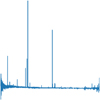 |
Fig. 5 Simple plot type of normalized spectra for one of the SDSS objects, a starburst Galaxy with ID 9068120565953615872. No axes are shown in the image as this is the exact plot fed into the ViT. |
 |
Fig. 6 Model pipeline example for a regression task: (a) data were obtained from surveys, (b) processed and kept in local files, (c) went through a generation of different plot types, and (d) passed through the ViT base model for fine-tuning. |
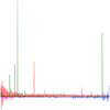 |
Fig. 7 Overlap plot type for spectra where each color channel of an RGB image contains one third of the normalized data. No axes are displayed as this is the exact plot fed into the ViT. |
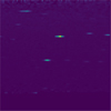 |
Fig. 8 2D map plot type of the spectra, where we associate each individual wavelength with a square of 3x3 pixels in the final plot. |
 |
Fig. 9 Overview of how each individual flux is mapped to the final 2D image in the 2D map design. Labels a, b, and c can be seen on the left in the standard flux plot, and in the right side with intensity set as the color of a given region in the image. |
6 Results
In this section we present the outcomes of our experiments and analyses. We begin by describing the evaluation metrics and datasets used for benchmarking. We then provide qualitative and quantitative results for both the classification and regression tasks. Finally, we compare our model’s performance against established baselines and discuss the implications of these findings.
The reported results are based on models fine-tuned on either the SLOMOST-Med or SLOMOST-Big datasets, as indicated in the description of each table. All models were fine-tuned for at least 30 epochs, with the best-performing checkpoint saved and used for evaluation. Hyperparameter tuning was conducted, and only the best results are shown. The optimal hyperparameters, a weight decay of 0.01 and a learning rate of 10−5, were selected based on the tuning results.
Performance results for the different image types from morphological classification.
Per-class recall for each different image type from morphological classification.
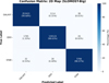 |
Fig. 10 2D map plot confusion matrix: predicted versus true labels (SLOMOST-Big). |
6.1 Classification results
Classification results are presented in Table 2 with overall accuracy and macro-averaged F1 scores for each type of input image. Table 3 shows per-class recall for each of these same image types. The fine-tuning was performed by minimizing the categorical cross entropy loss. For the 2D map representation, which achieved the best performance across the variants when fine-tuning on SLOMOST-Med, we also report results for SLOMOST-Big and present a confusion matrix in Figure 10.
6.2 Redshift estimation results
We present analogous results for the redshift regression task. Table 4 eports the R2 scores for each input image type, including results for the 2D map representation trained on SLOMOST-Big. We also include results with the simple 1D transformer as a baseline reference. Figure 11 shows the plot of predicted versus true redshift with 2D map when fine-tuning with SLOMOST-Big.
Table 5 summarizes the model performance in various S/N bins. Following the evaluation criteria proposed in Ross et al. (2020), we define a non-catastrophic redshift estimation as one in which the difference between predicted and true redshift corresponds to a velocity offset smaller than 3000 km s−1 for quasars and 1000 km s−1 for galaxies and stars; that is, where Δz, which is the absolute difference between predicted and true redshift, remains below these thresholds. Performance starts to drop in higher S/N bins, but that matches a significant drop in the amount of objects available for evaluation in them (e.g., only 0.02% of objects fall in the >50 S/N bin).
Performance results for the different image types from redshift regression.
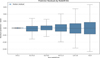 |
Fig. 11 Residuals of model predictions displayed as box plots across true redshift bins. Each box spans the interquartile range (25th–75th percentiles) of the residual distribution within that bin, whiskers extend to the 5th and 95th percentiles. Prediction results from regression with 2D map over SLOMOST-Big. |
6.3 Results on stellar parameters
Finally, we report R2 for three stellar parameter regression tasks, with ground truth being obtained from the SDSS DR18 directly and from LAMOST by merging information provided from their stellar parameter catalog of A, F, G, and K Stars. Results in this session contain only the subset of the datasets that pertain to stars, with all quasars and galaxies removed. Tables 6 and 7 present results for Teff and log g, respectively, where the simple plot yielded the best performance. Table 8 reports the [Fe/H] regression results, for which the overlap plot provided superior outcomes.
Performance of redshift regression over different S/N ranges with a 2D map.
Performance results for the different image types from effective temperature regression.
Performance results for the different image types from surface gravity regression.
Performance results for the different image types from metallicity regression.
7 Discussion
Our experiments show that converting astronomical spectra into 2D image formats enables ViTs to effectively capture both global and local spectral features. Among the representations explored, the 2D map format consistently demonstrated strong performance across tasks, although it did not outperform all alternatives in every setting, as can be seen in the previous section.
While the simple 1D transformer processes spectral sequences directly without information loss from image conversion, it is trained from scratch on the limited spectral dataset with minimal hyperparameter tuning. In contrast, ViTs leverage rich feature representations learned from millions of natural images through pretraining, which transfer effectively to 2D spectral visualizations. The current performance gap may reflect both the advantages of transfer learning and the limited architectural exploration of the 1D approach; further optimization of the transformer architecture, training strategies, and data augmentation techniques could potentially narrow this gap and better assess the relative merits of direct sequence processing versus pretrained vision models for spectral regression tasks.
Table 9 compares the performance of redshift regression in our model against the Bayesian SZNet model introduced by Podsztavek et al. (2022), as well as a simpler baseline model they implemented, Bayesian FCNN. The results for Bayesian SZNet are taken directly from their publication and are based on spectra exclusively from quasars in the SDSS DR 12. For our work, we report results both on the quasar-only subset and on the full test set, which includes objects from both SDSS and LAMOST, using the test portion of the SLOMOST-Big dataset. To enable comparison with Podsztavek et al. (2022), which only reported the continuous ranked probability score (CRPS), we computed the CRPS under a Gaussian assumption; the predicted values were treated as the means of Gaussian distributions, and the standard deviation was estimated from the residuals between predictions and ground-truth labels.
Compared to AstroCLIP, which reports an R2 of 0.990 for redshift regression using its spectrum encoder, we achieved a similar performance with an R2 of 0.992. Notably, our model was trained and evaluated on a substantially larger and more diverse dataset. The AstroCLIP encoder was trained over 500 epochs in a single day on approximately 200 000 spectra using four NVIDIA H100 GPUs. In contrast, we performed fine-tuning over nine days on a single NVIDIA 4090 GPU, using spectra from more than 14M objects. Normalizing for computational throughput (H100: 989 TFLOPS FP16, 4090: 330 TFLOPS FP16), our approach required approximately 72 H100-equivalent GPU hours compared to AstroCLIP’s 96 GPU hours, while processing 70 times more spectra. Moreover, the NVIDIA 4090 is significantly more accessible and affordable than H100 hardware, making our approach practical for researchers without access to large-scale computing infrastructure.
For classification, we compared our results to those of the SVM classifier from Wang et al. (2022), which was trained on a dataset that partially overlaps with the one used by us. Table 10 reports the accuracy of our model on our test set, alongside the accuracy of their SVM model and several other classification approaches evaluated in their study.
In the classification task, our model achieved near-perfect performance, reaching 99.0% accuracy on the SLOMOST-Med and SLOMOST-Big datasets when using the 2D map representation. Confusion matrices reveal that this representation particularly reduces misclassifications between quasars and galaxies, a category where less-processed formats such as the simple and overlap plots exhibited greater confusion. We attribute this improvement to 2D map’s capacity to more clearly emphasize spatial differences between emission- and absorption-line features, which are essential for distinguishing among object types.
For redshift regression, the ViT architecture benefited from its ability to model long-range dependencies within spectral structure. We achieved an R2 score of 0.992 on the diverse SLOMOST-Big dataset, indicating strong generalization across multiple source types, spectral ranges, and observational conditions. The model also maintained high accuracy across a wide range of S/Ns, with the best performance occurring at intermediate S/N values. The decline in performance at very high S/N levels may reflect limited sample sizes in those bins, although this trend merits further investigation.
Regression of stellar parameters observed lower R2 values than redshift regression overall but they were still meaningful. The simple and overlap representations often yielded better performance than the 2D map, particularly for Teff and log g. The relatively lower performance of the 2D map in these cases may indicate challenges in encoding subtle spectral features that influence these parameters. These observations suggest that targeted architectural adaptations, such as attention mechanisms incorporating spectral priors or hybrid image-sequence models, may be beneficial for improving performance in stellar parameter regression tasks. Additionally, stellar parameter inference presents unique difficulties, as ground-truth values from spectroscopic pipelines depend on theoretical stellar models that have known limitations and may not capture all relevant physical processes, introducing uncertainty into the training labels themselves (Candebat et al. 2024; Ness 2018).
In comparisons with baseline models, our model demonstrated competitive or superior performance as seen in the previous sections. Though we were not able to reproduce the exact results from the other studies given the availability and ease of reproduction, we used similar datasets and made observations of where they differ. For redshift regression, it outperformed Bayesian SZNet on diverse test sets, while achieving similar CRPS scores on quasar-only data. In classification, it surpassed several conventional machine-learning approaches, including SVMs and RFs, by achieving higher accuracy on overlapping datasets. Notably, these results were obtained using a single ViT-based architecture with minimal task-specific tuning, which supports the potential of this work as a general-purpose framework for spectral analysis.
In summary, the results highlight both the strengths and limitations of applying ViT-based models to spectroscopic data. While we achieved strong results in classification and redshift estimation, stellar parameter regression presents additional challenges that may require further methodological refinement. Future work could explore the integration of domain-specific knowledge into model architectures or the use of multimodal inputs that combine image representations with tabular or sequence-based data. As spectroscopic surveys continue to scale, newer models based on ViTs offer a promising foundation for efficient and accurate analysis of large volumes of spectral data.
Redshift regression performance of 2D map versus Bayesian SZNet.
Classification accuracy of multiple models from Wang et al. (2022) versus 2D map.
8 Conclusion and future work
In this work, we applied ViTs to perform several astronomical tasks, leveraging a novel framework for analyzing astronomical spectral data using pretrained ViTs. By transforming 1D spectra into 2D image representations and leveraging pretrained ViT backbones, we demonstrate that this approach can effectively capture complex spectral features and yield strong performance in both classification and regression tasks, offering a flexible and modular foundation for further experimentation and downstream applications in spectral analysis.
Our results highlight the potential for adapting modern deeplearning architectures to the challenges of astrophysical data, where the volume, heterogeneity, and complexity of observations continue to grow. By bridging the gap between traditional spectral formats and ViT-based models, this work enables a more scalable and accurate analysis of large datasets. This work represents a step toward the development of general-purpose tools for spectral science, contributing to the broader goal of advancing our understanding of the composition, structure, and evolution of the Universe.
Looking ahead, several directions for extension and refinement are available. These can be grouped into the following categories:
Model improvements: future work includes incorporating additional spectral datasets from surveys not yet covered in this study, exploring alternative image representations, and experimenting with enriched visual encodings. For example, multichannel spectral plots inspired by the overlap format could include first derivatives, continuum-subtracted flux, or line-detection maps. In addition, we plan to explore multimodal architectures, such as those inspired by AstroCLIP, that combine spectral data with complementary metadata or photometric information;
Extended downstream tasks: beyond coarse classification and redshift estimation, future work could involve fine-grained stellar or galaxy subclassification, as well as anomaly-detection tasks for identifying rare or unusual spectral types. These directions will require the model to learn more nuanced spectral cues and may benefit from specialized loss functions or attention mechanisms;
Architectural refinements: further experiments are planned to evaluate changes in the ViT architecture itself, including variations in patch size, transformer depth, and token pooling strategies. Although initial attempts at pretraining ViTs from scratch on spectroscopic data did not yield notable gains, more targeted pretraining or contrastive learning approaches may improve generalization;
Cross-domain applications: we also intend to explore applications of this framework outside of astronomy. In fields such as agriculture, environmental monitoring, or materials science, spectral measurements are commonly used for classification or regression tasks. Our domain-agnostic structure and modular pipeline make it a promising candidate for transfer to these domains, provided appropriate training data are available.
Overall, this work lays the groundwork for more flexible, accurate, and scalable spectral analysis pipelines. We hope it contributes to the development of new machine-learning techniques and practical tools for the next generation of spectroscopic surveys and beyond.
Data availability
All of the source code for these experiments can be found at https://github.com/astromer-science/spectromer, and we welcome contributions and feedback. Metadata files for both of the surveys used here are also provided, as well as documentation on how to introduce data from a new survey.
Acknowledgements
Funding for the Sloan Digital Sky Survey V has been provided by the Alfred P. Sloan Foundation, the Heising-Simons Foundation, the National Science Foundation, and the Participating Institutions. SDSS acknowledges support and resources from the Center for High-Performance Computing at the University of Utah. SDSS telescopes are located at Apache Point Observatory, funded by the Astrophysical Research Consortium and operated by New Mexico State University, and at Las Campanas Observatory, operated by the Carnegie Institution for Science. The SDSS web site is www.sdss.org. SDSS is managed by the Astrophysical Research Consortium for the Participating Institutions of the SDSS Collaboration, including Caltech, The Carnegie Institution for Science, Chilean National Time Allocation Committee (CNTAC) ratified researchers, The Flatiron Institute, the Gotham Participation Group, Harvard University, Heidelberg University, The Johns Hopkins University, L’Ecole polytechnique fédérale de Lausanne (EPFL), Leibniz-Institut für Astrophysik Potsdam (AIP), Max-Planck-Institut für Astronomie (MPIA Heidelberg), Max-Planck-Institut für Extraterrestrische Physik (MPE), Nanjing University, National Astronomical Observatories of China (NAOC), New Mexico State University, The Ohio State University, Pennsylvania State University, Smithsonian Astrophysical Observatory, Space Telescope Science Institute (STScI), the Stellar Astrophysics Participation Group, Universidad Nacional Autónoma de México, University of Arizona, University of Colorado Boulder, University of Illinois at Urbana-Champaign, University of Toronto, University of Utah, University of Virginia, Yale University, and Yunnan University. Guoshoujing Telescope (the Large Sky Area Multi-Object Fiber Spectroscopic Telescope LAMOST) is a National Major Scientific Project built by the Chinese Academy of Sciences. Funding for the project has been provided by the National Development and Reform Commission. LAMOST is operated and managed by the National Astronomical Observatories, Chinese Academy of Sciences. GCV acknowledges support from the National Agency for Research and Development (ANID) grants: Millennium Science Initiative ICN12_009, AIM23-0001, NCN2021_080, NCN2024_112, and FONDECYT Regular 1231877.
References
- Astropy Collaboration (Price-Whelan, A. M., et al.) 2022, ApJ, 935, 167 [NASA ADS] [CrossRef] [Google Scholar]
- Breiman, L. 2001, Mach. Learn., 45, 5 [Google Scholar]
- Burrows, A., & Orton, G. 2010, in Exoplanets, ed. S. Seager (Tucson: University of Arizona Press), 419 [Google Scholar]
- Campbell, R. J., Mathioudakis, M., & Quintero Noda, C. 2026, ApJ, 996, 63 [Google Scholar]
- Candebat, N., Sacco, G. G., Magrini, L., et al. 2024, A&A, 692, A228 [NASA ADS] [CrossRef] [EDP Sciences] [Google Scholar]
- Cao, J., Xu, T., Deng, Y., et al. 2024, A&A, 683, A42 [NASA ADS] [CrossRef] [EDP Sciences] [Google Scholar]
- Caron, M., Touvron, H., Misra, I., et al. 2021, in 2021 IEEE/CVF International Conference on Computer Vision (ICCV), 9630 [Google Scholar]
- Cenarro, A. J., Moles, M., Cristóbal-Hornillos, D., et al. 2019, A&A, 622, A176 [NASA ADS] [CrossRef] [EDP Sciences] [Google Scholar]
- Chaplin, W. J., & Miglio, A. 2013, ARA&A, 51, 353 [Google Scholar]
- Cho, K., van Merriënboer, B., Gulcehre, C., et al. 2014, in Proceedings of the 2014 Conference on Empirical Methods in Natural Language Processing (EMNLP), eds. A. Moschitti, B. Pang, & W. Daelemans (Doha, Qatar: Association for Computational Linguistics), 1724 [Google Scholar]
- Colless, M., Dalton, G., Maddox, S., et al. 2001, MNRAS, 328, 1039 [Google Scholar]
- Cortes, C., & Vapnik, V. 1995, Mach. Learn., 20, 273 [Google Scholar]
- Creevey, O. L., Sordo, R., Pailler, F., et al. 2023, A&A, 674, A26 [NASA ADS] [CrossRef] [EDP Sciences] [Google Scholar]
- Daoutis, C., Zezas, A., Kyritsis, E., Kouroumpatzakis, K., & Bonfini, P. 2025, A&A, 693, A95 [NASA ADS] [CrossRef] [EDP Sciences] [Google Scholar]
- Dawson, K. S., Schlegel, D. J., Ahn, C. P., et al. 2013, AJ, 145, 10 [Google Scholar]
- Dawson, K. S., Kneib, J.-P., Percival, W. J., et al. 2016, AJ, 151, 44 [Google Scholar]
- de Jong, R. S., Barden, S. C., Bellido-Tirado, O., et al. 2016, in Ground-based and Airborne Instrumentation for Astronomy VI, 9908, eds. C. J. Evans, L. Simard, & H. Takami, International Society for Optics and Photonics (SPIE), 99081O [Google Scholar]
- Deng, J., Dong, W., Socher, R., et al. 2009, in 2009 IEEE Conference on Computer Vision and Pattern Recognition, 248 [Google Scholar]
- Devlin, J., Chang, M.-W., Lee, K., & Toutanova, K. 2019, in Proceedings of the 2019 Conference of the North American Chapter of the Association for Computational Linguistics: Human Language Technologies, 1 (Long and Short Papers), eds. J. Burstein, C. Doran, & T. Solorio (Minneapolis, Minnesota: Association for Computational Linguistics), 4171 [Google Scholar]
- Donoso-Oliva, C., Becker, I., Protopapas, P., et al. 2023, A&A, 670, A54 [NASA ADS] [CrossRef] [EDP Sciences] [Google Scholar]
- Dosovitskiy, A., Beyer, L., Kolesnikov, A., et al. 2021, in International Conference on Learning Representations [Google Scholar]
- Fischer, D. A., & Valenti, J. 2005, ApJ, 622, 1102 [NASA ADS] [CrossRef] [Google Scholar]
- Frontera-Pons, J., Sureau, F., Moraes, B., Bobin, J., & Abdalla, F. B. 2019, A&A, 625, A73 [NASA ADS] [CrossRef] [EDP Sciences] [Google Scholar]
- Gaia Collaboration (Prusti, T., et al.) 2016, A&A, 595, A1 [NASA ADS] [CrossRef] [EDP Sciences] [Google Scholar]
- Gray, D. F. 2005, The Observation and Analysis of Stellar Photospheres, 3rd edn. (Cambridge, UK: Cambridge University Press) [Google Scholar]
- Hahn, C., Wilson, M. J., Ruiz-Macias, O., et al. 2023, AJ, 165, 253 [CrossRef] [Google Scholar]
- Hochreiter, S., & Schmidhuber, J. 1997, Neural Comput., 9, 1735 [CrossRef] [Google Scholar]
- Hubble, E. 1929, PNAS, 15, 168 [CrossRef] [Google Scholar]
- Koblischke, N., & Bovy, J. 2024, in Neurips 2024 Workshop Foundation Models for Science: Progress, Opportunities, and Challenges [Google Scholar]
- Kollmeier, J., Anderson, S. F., Blanc, G. A., et al. 2019, in BAAS, 51, 274 [NASA ADS] [Google Scholar]
- Krizhevsky, A., Sutskever, I., & Hinton, G. E. 2012, in Advances in Neural Information Processing Systems, 25, 1097 [Google Scholar]
- Kügler, S. D., Polsterer, K., & Hoecker, M. 2015, A&A, 576, A132 [NASA ADS] [CrossRef] [EDP Sciences] [Google Scholar]
- LeCun, Y., Bottou, L., Bengio, Y., & Haffner, P. 1998, Proc. IEEE, 86, 2278 [Google Scholar]
- Luo, A.-L., Zhao, Y., Gang, Z., et al. 2015, Res. Astron. Astrophys., 15, 1095 [Google Scholar]
- Machado, D. P., Leonard, A., Starck, J. L., Abdalla, F. B., & Jouvel, S. 2013, A&A, 560, A83 [NASA ADS] [CrossRef] [EDP Sciences] [Google Scholar]
- Maiolino, R., & Mannucci, F. 2019, Astron. Astrophys. Rev., 27, 3 [Google Scholar]
- Majewski, S. R., Schiavon, R. P., Frinchaboy, P. M., et al. 2017, AJ, 154, 94 [NASA ADS] [CrossRef] [Google Scholar]
- Marchetti, A., Granett, B. R., Guzzo, L., et al. 2012, MNRAS, 428, 1424 [Google Scholar]
- Mészáros, S., Holtzman, J., García Pérez, A. E., et al. 2013, AJ, 146, 133 [Google Scholar]
- Ness, M. 2018, PASA, 35, e003 [NASA ADS] [CrossRef] [Google Scholar]
- Ness, M., Hogg, D. W., Rix, H.-W., Ho, A. Y. Q., & Zasowski, G. 2015, ApJ, 808, 16 [NASA ADS] [CrossRef] [Google Scholar]
- Parker, L., Lanusse, F., Golkar, S., et al. 2024, MNRAS, 531, 4990 [Google Scholar]
- Pattnaik, R., Kartaltepe, J. S., & Binu, C. 2025, ApJ, 988, 139 [Google Scholar]
- Podsztavek, O., Škoda, P., & Tvrdík, P. 2022, Astron. Comput., 40, 100615 [NASA ADS] [CrossRef] [Google Scholar]
- Preston, G. W. 1974, ARA&A, 12, 257 [Google Scholar]
- Pâris, I., Petitjean, P., Ross, N. P., et al. 2017, A&A, 597, A79 [NASA ADS] [CrossRef] [EDP Sciences] [Google Scholar]
- Radford, A., Wu, J., Child, R., et al. 2019, https://cdn.openai.com/better-language-models/language_models_are_unsupervised_ multitask_learners.pdf [Google Scholar]
- Ross, A. J., Bautista, J., Tojeiro, R., et al. 2020, MNRAS, 498, 2354 [NASA ADS] [CrossRef] [Google Scholar]
- Różański, T., Ting, Y.-S., & Jabłońska, M. 2025, ApJ, 980, 66 [Google Scholar]
- Schlegel, D., Dey, A., Herrera, D., et al. 2021, in American Astronomical Society Meeting Abstracts, 237, 235.03 [Google Scholar]
- Scodeggio, M., Guzzo, L., Garilli, B., et al. 2018, A&A, 609, A84 [NASA ADS] [CrossRef] [EDP Sciences] [Google Scholar]
- Sheinis, A., Barden, S. C., Sobeck, J., & the MSE Team. 2023, Astron. Nachr., 344, e20230108 [Google Scholar]
- Simonyan, K., & Zisserman, A. 2015, in International Conference on Learning Representations [Google Scholar]
- Stoughton, C., Lupton, R. H., Bernardi, M., et al. 2002, AJ, 123, 485 [Google Scholar]
- Vaswani, A., Shazeer, N., Parmar, N., et al. 2017, in Advances in Neural Information Processing Systems, 30, eds. I. Guyon, U. V. Luxburg, S. Bengio, et al. (Curran Associates, Inc.) [Google Scholar]
- Vavilova, I. B., Dobrycheva, D. V., Vasylenko, M. Y., et al. 2021, A&A, 648, A122 [NASA ADS] [CrossRef] [EDP Sciences] [Google Scholar]
- Wahlgren, G. M. 2011, Can. J. Phys., 89, 345 [Google Scholar]
- Wang, C., Bai, Y., López-Sanjuan, C., et al. 2022, A&A, 659, A144 [Google Scholar]
- Willett, K. W., Lintott, C. J., Bamford, S. P., et al. 2013, MNRAS, 435, 2835 [Google Scholar]
- Wolfe, A. M., Gawiser, E., & Prochaska, J. X. 2005, ARA&A, 43, 861 [Google Scholar]
- Yang, M., Wu, H., Yang, F., et al. 2018, ApJSS, 234, 5 [Google Scholar]
snMedian is a value provided by SDSS to represent an overall S/N value for the object across the different filter bands.
We computed snMedian as snMedian ![Mathematical equation: $\[=\sqrt{{\sum}_{i \in\{u, g, r, i, z\}} S / N_{i}^{2}}\]$](/articles/aa/full_html/2026/05/aa55748-25/aa55748-25-eq1.png) , following SDSS-derived practices.
, following SDSS-derived practices.
All Tables
Performance results for the different image types from morphological classification.
Per-class recall for each different image type from morphological classification.
Performance results for the different image types from effective temperature regression.
Performance results for the different image types from surface gravity regression.
Classification accuracy of multiple models from Wang et al. (2022) versus 2D map.
All Figures
|
Fig. 1 Vision transformer architecture. An input image is divided into fixed-sized patches, which are linearly embedded and combined with positional encodings before being processed through transformer encoder layers. Figure sourced from Dosovitskiy et al. (2021). |
| In the text | |
|
Fig. 2 Distribution of redshifts for the SDSS dataset. |
| In the text | |
|
Fig. 3 Distribution of redshifts for the LAMOST dataset. |
| In the text | |
|
Fig. 4 Comparison of snMedian distributions across both datasets via a log-scale box plot. The central box spans the interquartile range (25th–75th percentiles), whiskers extend to the 5th and 95th percentiles, and outliers beyond this range are omitted for clarity. |
| In the text | |
|
Fig. 5 Simple plot type of normalized spectra for one of the SDSS objects, a starburst Galaxy with ID 9068120565953615872. No axes are shown in the image as this is the exact plot fed into the ViT. |
| In the text | |
|
Fig. 6 Model pipeline example for a regression task: (a) data were obtained from surveys, (b) processed and kept in local files, (c) went through a generation of different plot types, and (d) passed through the ViT base model for fine-tuning. |
| In the text | |
|
Fig. 7 Overlap plot type for spectra where each color channel of an RGB image contains one third of the normalized data. No axes are displayed as this is the exact plot fed into the ViT. |
| In the text | |
|
Fig. 8 2D map plot type of the spectra, where we associate each individual wavelength with a square of 3x3 pixels in the final plot. |
| In the text | |
|
Fig. 9 Overview of how each individual flux is mapped to the final 2D image in the 2D map design. Labels a, b, and c can be seen on the left in the standard flux plot, and in the right side with intensity set as the color of a given region in the image. |
| In the text | |
|
Fig. 10 2D map plot confusion matrix: predicted versus true labels (SLOMOST-Big). |
| In the text | |
|
Fig. 11 Residuals of model predictions displayed as box plots across true redshift bins. Each box spans the interquartile range (25th–75th percentiles) of the residual distribution within that bin, whiskers extend to the 5th and 95th percentiles. Prediction results from regression with 2D map over SLOMOST-Big. |
| In the text | |
Current usage metrics show cumulative count of Article Views (full-text article views including HTML views, PDF and ePub downloads, according to the available data) and Abstracts Views on Vision4Press platform.
Data correspond to usage on the plateform after 2015. The current usage metrics is available 48-96 hours after online publication and is updated daily on week days.
Initial download of the metrics may take a while.