| Issue |
A&A
Volume 708, April 2026
|
|
|---|---|---|
| Article Number | A335 | |
| Number of page(s) | 8 | |
| Section | Interstellar and circumstellar matter | |
| DOI | https://doi.org/10.1051/0004-6361/202659248 | |
| Published online | 22 April 2026 | |
Charge-aware machine learning for the infrared spectra of interstellar polycyclic aromatic hydrocarbons
Laboratory for Relativistic Astrophysics, Department of Physics, Guangxi University,
530004
Nanning,
China
★ Corresponding author: This email address is being protected from spambots. You need JavaScript enabled to view it.
Received:
31
January
2026
Accepted:
20
March
2026
Abstract
Aims. Polycyclic aromatic hydrocarbons (PAHs) are among the most abundant molecules in the interstellar medium. Their characteristic infrared (IR) emission acts as a sensitive probe of astrophysical environments, yet detailed spectral analyses have been limited by the high computational cost of density functional theory (DFT) calculations. This constraint has hindered a systematic exploration of how spectral features such as the aromatic IR bands depend on a PAH's charge state and molecular structure.
Methods. Our goal is to develop a computationally efficient machine learning model capable of predicting IR spectra for PAHs across charge states, and to critically reassess established interpretations of how ionization influences these spectra.
Results. We developed a neural network framework to predict PAH IR spectra across four charge states, utilizing a dataset of 12599 species. Molecular structures were represented by topological fingerprints, with charge states integrated via learnable embeddings. Additionally, a random forest classifier was implemented to infer charge states directly from spectral data.
Conclusions. The model achieves near-DFT accuracy in predicting IR spectra while offering orders-of-magnitude acceleration in computation. It reliably handles PAHs containing up to 150 carbon atoms, including anions, neutrals, cations, and di-cations. The predictive capability for larger molecules is currently limited by the available training data. The classifier predicts charge states with over 99% accuracy. Our analysis of the DFT-computed spectra shows that anions exhibit strong emission across multiple bands, often matching or exceeding cation intensities, and the 11.2 micrometer band shows a distinct charge dependence.
Key words: methods: laboratory: molecular / ISM: molecules
© The Authors 2026
 Open Access article, published by EDP Sciences, under the terms of the Creative Commons Attribution License (https://creativecommons.org/licenses/by/4.0), which permits unrestricted use, distribution, and reproduction in any medium, provided the original work is properly cited.
This article is published in open access under the Subscribe to Open model. This email address is being protected from spambots. You need JavaScript enabled to view it. to support open access publication.
1 Introduction
Polycyclic aromatic hydrocarbons (PAHs), planar molecules composed of fused carbon rings, are abundant throughout the interstellar medium (Allamandola et al. 1989). When excited by ultraviolet photons, they fluoresce in the infrared (IR), producing the well-known aromatic infrared bands (AIBs) at approximately 3.3, 6.2, 7.7, 8.6, and 11.2 μm (Tielens 2008). These bands serve as sensitive tracers of physical conditions because their shapes and intensities depend strongly on the local environment, particularly the PAHs' charge state and size distribution (Peeters et al. 2002; van Diedenhoven et al. 2004).
Charge plays a central role: ionized PAHs emit orders of magnitude more strongly in the 6–9 μm region than their neutral counterparts and exhibit systematic spectral shifts that help explain the multi-peak structure of the 7.7 μm complex (Allamandola et al. 1999; Bauschlicher et al. 2008; Ricca et al. 2012). At the same time, structural details such as edge configuration, heteroatom inclusion, and defects modulate the spectral response to charge, adding further complexity (e.g., Bauschlicher et al. 2009; Ricca et al. 2021, 2024; Li et al. 2024; Yang et al. 2021). Interpreting AIBs therefore requires understanding the coupled effects of charge and molecular geometry across a vast chemical landscape (Peeters et al. 2021; Li 2020).
The NASA Ames PAH IR spectroscopic database (PAHdb) provides a foundation for such studies, containing computed and experimental spectra for over ten thousand PAHs in multiple charge states (Boersma et al. 2014; Bauschlicher et al. 2018; Mattioda et al. 2020; Ricca et al. 2026). This high-fidelity dataset has catalyzed large-scale investigations and more comprehensive analyses of AIBs (e.g., Andrews et al. 2015; Shannon et al. 2016; Maragkoudakis et al. 2020, 2025). Despite these advancements, existing database entries represent only a fraction of the structural diversity expected in the interstellar medium, a limitation largely imposed by the steep computational scaling of quantum chemical calculations as molecular size increases.
To bypass this computational bottleneck, we previously developed a machine learning (ML) framework capable of predicting PAH spectra with near-quantum-chemical accuracy at a fraction of the traditional cost (Kovács et al. 2020). This approach pioneered the application of ML to spectral prediction for various molecular systems (e.g., McGill et al. 2021; Laurens et al. 2021; Calvo et al. 2021; Stienstra et al. 2025) and offered a more comprehensive understanding of the complex relationship between molecular structure and astronomical spectra (Meng et al. 2021, Meng et al. 2023). However, that model utilized a topological fingerprint that lacked explicit charge encoding. In the present work, we address this critical gap by introducing a charge-aware extension. Our revised architecture not only integrates charge-state information but also systematically evaluates different encoding strategies to optimize predictive performance.
2 Methods
Our methodology follows a unified workflow integrating data construction, spectral processing, and model validation. We compile a set of PAH IR spectra from density functional theory (DFT) calculations and the PAHdb, discretizing them into histograms. Molecules are represented by molecular fingerprints augmented with charge-state information. Using these features, a neural network (NN) model is trained to predict IR spectra, with performance assessed through cross-validation and testing. Additionally, a random forest (RF) classifier is trained on the IR spectra to evaluate the correlation between the charge states and spectral signatures.
2.1 Data collection
To construct a systematic dataset of PAH spectra, we began with a self-generated library of over one million distinct PAH structures. We selected 1155 representative hydrocarbon PAHs by maximizing the separation of their Perron roots (the largest eigenvalues of their molecular distance matrices) in eigenspectrum space, ensuring broad structural diversity.
The IR spectra of each selected structure were computed for three charge states: anionic (−1), neutral (0), and cationic (+1). Calculations were performed using DFT with the B3LYP functional (Stephens et al. 1994), as implemented in Gaussian 16 B.01 (Frisch et al. 2016; Liao et al. 2023; Lu et al. 2021). For all open-shell species (anions and cations), the unrestricted B3LYP (UB3LYP) formalism was automatically employed to correctly account for spin polarization. This level of theory is well suited for ionized aromatic systems; specifically, the 6-311+G(d,p) basis set includes diffuse functions that are essential for the extended electronic distributions of anions, while the triple-zeta valence and polarization functions are critical for accurately capturing the delocalized π-electron density and vibrational modes that produce key IR features. Furthermore, the unrestricted approach ensures an accurate description of electronic structures potentially influenced by Jahn-Teller distortions in radical species. The resulting 3465 harmonic spectra were uniformly scaled by a factor of 0.9757, following established recommendations for PAH spectroscopy (Bauschlicher & Langhoff 1997). Note that our self-generated DFT dataset includes three charge states (–1, 0, and +1), while the PAHdb additionally provides di-cations (+2).
To validate the selected level of theory, we benchmarked our computational framework against a representative subset of 84 PAHs with available experimental spectra in the PAHdb. Ten illustrative examples are shown in Appendix A, spanning five distinct intervals of prediction error from high-fidelity to poor agreement. It is confirmed that our DFT-based spectra align closely with experimental references, thereby ensuring that the ML models subsequently learn physically meaningful relationships between molecular structure and vibrational features.
To enhance the model's generalizability, we augmented our dataset with 9731 theoretical (harmonic, scaled) spectra from the PAHdb (v4.0), which include PAHs with heteroatoms of oxygen and nitrogen. These encompass four charge states: anionic, neutral, cationic, and di-cationic (–1, 0, +1, and +2). Tri-cationic PAHs available in the PAHdb were not selected due to insufficient data for the model to learn meaningful spectral-structure relationships. For the same reason, we also excluded dehydrogenated, hyper-hydrogenated, silicon-containing and metal-containing species. After merging and de-duplication with the 3465 spectra, the final consolidated dataset comprised 12 599 species. The size and charge distributions of these PAHs are presented in Fig. 1. To prevent data leakage, we verified that no duplicate structures exist in the dataset. By encoding molecules into fingerprint fragments, the model maps local chemical environments to spectral features rather than memorizing global identities, ensuring that predictive accuracy stems from learned physical correlations rather than scaffold overlap or data leakage.
Each computed spectrum was converted to an intensity histogram using a bin width of 11.88 cm–1, determined by Knuth's Bayesian rule (Knuth 2006), which optimizes bin size by balancing detail retention against model complexity to avoid overfitting. The resulting histogram spans 6.95–5376 cm−1 with 300 bins. A sensitivity test confirms that shifting the lower bound to 100 cm−1 yields negligible changes in model performance, whereas narrower bin widths degrade predictive accuracy.
We split each histogram at the 147th bin (1753 cm−1), which corresponds to a spectral gap common to all PAHs. This threshold separates collective skeletal vibrations below it from localized hydrogen-atom stretching modes above it. The two sub-histograms: low-frequency (≤1753 cm−1) and high-frequency (>î753 cm−1), were independently normalized to unit sum, yielding two probability-like intensity distributions per spectrum. These serve as the prediction targets for the ML spectrum predictor.
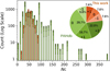 |
Fig. 1 Distribution of carbon-atom counts (NC, in log scale) for PAHs in our generated dataset (orange bars) and for those selected from the PAHdb (green bars). The stacked segments within each bar represent different charge states. |
2.2 Feature engineering
2.2.1 Molecular structure descriptor
For model input, the topological structure of each molecule was encoded using the extended-connectivity fingerprints (ECFPs; Morgan 1965). Implemented via the RDKit chem-informatics toolkit1, ECFPs generate a fixed-length vector representation by systematically enumerating circular substructures up to a specified bond radius from each atom and hashing them into unique identifiers (Li et al. 2026). Each element in the resulting fingerprint corresponds to a specific molecular fragment and records its frequency of occurrence within the molecule.
For this work, a radius cutoff of 11 bonds was selected to achieve high structural resolution. To reduce noise and improve generalization, only fingerprint features that appeared in at least four molecules in the training set were retained. This filtering resulted in 42 535 unique molecular fragments across the entire PAH dataset, which served as the final feature set for model training.
2.2.2 Charge-state descriptor
Molecular charge-state information was integrated using two distinct schemes:
Learnable embedding: discrete charge values were mapped to a 16-dimensional dense vector via a trainable embedding layer. This embedding was optimized jointly with the neuron weights, enabling the model to learn how charge modulates spectral features such as peak shifts, intensities, and band broadening, in a nonlinear, data-driven manner.
One-hot encoding: charge states were treated as categorical variables and encoded into four-dimensional one-hot vectors (representing −1, 0, +1, and +2). This sparse representation provides an explicit, fixed indicator of electronic state that distinguishes otherwise topologically identical molecules in different charge states.
These two charge-state representations were separately combined with ECFP to serve as inputs for the ML spectrum predictor. In addition, we also implemented a third, dual-input model that directly passed the raw scalar charge value (without encoding) and the ECFP fingerprint through separate fully connected layers before concatenation and final prediction. However, this model performed significantly worse than the learnable-embedding and one-hot encoding models, and is therefore omitted from further discussion.
2.3 Neural network spectrum predictor
2.3.1 Architecture
A fully connected multilayer perceptron NN was used for spectral prediction. It consists of four hidden layers with dimensions 1500, 1000, 800, and 600 neurons, progressively reducing feature dimensionality to encourage abstraction. Rectified linear unit activation functions were applied after each hidden layer to alleviate vanishing gradients and promote faster convergence. The output layer dimension matches the resolution of the discretized target spectra. To ensure physically meaningful predictions, an absolute value operation was applied to the final layer, enforcing non-negative spectral intensities. The model was optimized using the Adam optimizer with an initial learning rate of 0.0001 and a batch size of 32.
The earth mover's distance (EMD) was used as the loss function for spectral prediction, as it is sensitive to peak position and shape, unlike pointwise metrics like mean absolute error, by penalizing cumulative mismatches across the entire spectrum. This encourages structural alignment between predicted and true spectra. The EMD, validated in prior spectral work, measures the minimal "work" to transform one distribution into another, providing robustness to small peak shifts. For normalized spectra a and b, the EMD is defined as the L1 distance between their cumulative distribution functions:  .
.
2.3.2 Training, evaluation, and validation
The dataset was randomly split into training, validation, and test subsets in a ratio of 6:2:2. An early stopping mechanism with a patience of 50 epochs was applied during training to prevent overfitting, halting the process if the validation EMD loss showed no significant improvement and restoring the model weights associated with the best validation performance.
Generalization ability was further evaluated through a group five-fold cross-validation. In each fold, the data were partitioned so that one subset served as the test set, another as the validation set (with early stopping applied), and the remaining three as the training set. Final performance metrics were averaged across all five folds to ensure robustness and reliability.
To ensure reproducibility, the complete source code for the model, along with the training and testing datasets, is openly available at the Git repository: ChargeEncoding-IRPrediction.
2.4 Random forest charge-state classifier
To further investigate the relationship between spectral features and ionization, we trained a RF classifier to predict charge labels directly from binned IR spectra generated by our DFT calculations. This was treated as a three-class classification problem: anion (−1), neutral (0), and cation (+1). The dataset was split into training and test sets using an 8:2 ratio, ensuring a balanced class representation.
The central objective of this classification was to calculate feature importance scores, which quantify the contribution of each input variable, specifically, individual spectral bins to the model's predictive accuracy. By analyzing these scores, we can identify specific vibrational frequencies that serve as "fingerprints" for charge states. This approach allows us to bridge the gap between ML performance and physical interpretation, mapping the model's decision-making process back to critical spectral bands associated with molecular charge.
3 Results and discussion
3.1 Statistic and ML analyses of DFT results
To establish a reliable spectroscopic benchmark, we first validated our dataset through a systematic comparison of our DFT-calculated spectra with literature results. Figure 2 presents a statistical analysis of the DFT-computed spectra for 3465 PAHs across neutral, cationic, and anionic states. Panel a shows normalized mean spectra, highlighting that charge state is a primary determinant of the IR profile. PAH IR spectra are highly sensitive to specific structural motifs; therefore, different sample populations lead to different statistical conclusions. While the findings of our studied PAHs align with general charge-dependent trends, we identify specific deviations from earlier benchmarks, as detailed below.
The 3.3 μm band (Panel b) arises from aromatic C-H stretching. While literature reports have established foundational benchmarks for band intensity based on specific neutral samples (Allamandola et al. 1999; Bakes et al. 2001; Hudgins et al. 2001; Draine & Li 2007), our results derived from a consistent analysis of an expanded population suggest a statistically distinct intensity order of anion > neutral > cation. Peak positions in (Panel h), anion (3.240 μm) > neutral (3.222 μm) > cation (3.206 μm), suggest that the wavelength distribution is governed more strongly by charge than by specific geometry (Bauschlicher et al. 2009, 2018). These dataset-specific trends suggest that the statistical mean of spectral properties can shift when moving from small, specific molecular groups to the high-dimensional structural diversity represented in this work.
For the 6.2 μm band (Panel c), typically a tracer of ionic states (Allamandola et al. 1999; Peeters et al. 2002; Maragkoudakis et al. 2025), we find negligible neutral contributions. However, our observed intensity order (anion > cation > neutral) and nearly identical peak wavelengths suggest a need to reassess the conventional view of this band as a purely cationic marker, indicating that anions can also be dominant contributors within large, heterogeneous PAH populations.
The 7.7 μm band (Panel d), attributed to C-C stretching (Draine & Li 2001, 2007), is often regarded as cation-dominated (Bauschlicher et al. 2008). While we confirm minimal neutral contribution and an anionic redshift (Panel j), our observed intensity hierarchy indicates that this band is not exclusively dominated by cations when considering the full structural diversity of the current dataset. Significant error bars in Panel j suggest that the redshift magnitude is sensitive to specific molecular geometry.
The 8.6 μm band (Panel e), typically correlated with the C-H in-plane bending mode, is characteristically enhanced in ionic species (Allamandola et al. 1999; Ricca et al. 2018). We confirm a clear intensity hierarchy (anion > cation > neutral) with no systematic peak shifts (Panel k).
For the 11.2 μm band (Panel f), it is reported that neutral PAHs exhibit the strongest intensity (Draine & Li 2007; Maragkoudakis et al. 2020). In contrast, our systematic analysis of over 3000 species provides a different statistical profile, where the intensities across all three charge states appear more comparable than previously reported for smaller subsets. Furthermore, the summed spectra in Panel (1) confirm that cations exhibit a systematic blueshift relative to neutrals.
The 12.5–14.5 μm region (Panel g) encompasses duo, trio, and quartet C-H out-of-plane (OOP) bending modes (Hony et al. 2001; Peeters et al. 2017). While we confirm the peak wavelength trend of anion > neutral > cation (Panel m), the shifts are relatively subtle in this dataset. Moreover, a distinct intensity hierarchy of anion > cation > neutral suggests that anions produce pronounced spectral signatures in this complex region for large PAH populations (Bauschlicher et al. 2009).
To further elucidate the relationship between IR spectra and PAH ionization states, we performed a feature importance analysis using the RF classifier described in Sect. 2.4. The model effectively captured the correlations between spectral features and molecular charge, achieving a classification accuracy of nearly 1.0 (Table 1, left). By ranking the resulting importance scores, we established a mapping between specific vibrational modes and electrostatic states, identifying the diagnostic IR bands most critical for charge-state determination. These results, visualized in Table 1 (right), highlight the spectral regions that serve as the primary "fingerprints" for distinguishing between anion, neutral, and cation species.
For neutral molecules, the ML model agrees with prior studies in identifying the strong absorption at 3.3 μm as a primary diagnostic. Additionally, it incorporates the ion-enhanced emission pattern in the 6–9 μm range (Peeters et al. 2002), using the absence of signal at 7.6 μm as a supporting negative marker. In the case of anions, while Bauschlicher et al. (2008, 2009) emphasizes enhancements near 7.7 and 8.6 μm, the RF model selects the 7.75 μm band. Owing to the noted sensitivity of the 8.6 μm peak center to structural variations (Ricca et al. 2018), the model shifts focus to the more stable red-wing region at 8.9 μm and the OOP edge at 11.7 μm. For cations, ML model highlights a previously underappreciated secondary feature at 9.8 μm (ranked second in feature importance). This band typically falls within the spectral region associated with C-H OOP bending vibrations, a finding consistent with theoretical studies on PAH cations (Bauschlicher et al. 2008).
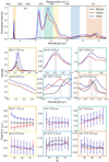 |
Fig. 2 Statistical analysis of IR spectra for 3465 PAHs in neutral (black), cationic (red), and anionic (blue) states. (a) Mean spectra from 2.5 to 15 μm. Shaded regions highlight key AIBs. (b)–(g) Close-ups of major bands with peak positions marked. (h)-(m) Peak position vs. carbon atom count (NC). Points show binned averages, and error bars are standard deviations. |
3.2 ML prediction of IR spectra
The above analysis of DFT-computed spectra demonstrates that ML can effectively capture the influence of the charge state on the PAH IR spectra. In this subsection we evaluate the ability of our NN model (described in Sect. 2.3) to predict the IR spectra of 12 599 PAHs across four distinct charge states: −1,0, +1, and +2, benchmarking predictions against reference DFT calculations. To evaluate the influence of the model's output representation, we first compared models trained on relative (normalized) versus absolute spectral intensities.
Table 2 lists the average EMD errors categorized by charge state. The prediction of relative intensities consistently yields lower errors across all ionization categories. This is anticipated as learning normalized spectral profiles aligns naturally with a shape-based metric like the EMD. Conversely, predicting absolute intensities imposes the significantly more complex regression task of reproducing the total oscillator strength, which exhibits substantial variation across molecules (Ramakrishnan et al. 2015).
The second key observation from Table 2 is the nonmonotonic relationship between data size and prediction accuracy for charged species. While the largest subset (neutral, N = 4571) has the lowest error (mean EMD = 2.47), the smaller di-cation dataset (N = 2776) yields better accuracy (2.52) than the larger cation set (2.81, N = 3066). This likely reflects the increased physical complexity of charged species. Cationic and di-cationic PAHs often undergo greater structural distortion (e.g., Jahn-Teller effects) and exhibit altered electron correlation (Jahn & Teller 1937; Eisenberg & Shenhar 2012), leading to more complex potential energy surfaces and inherently more challenging vibrational spectra to model.
Given the superior performance of the relative intensity model, we used it for a detailed evaluation of different charge-encoding strategies. Figure 3 compares prediction errors for the low- and high-frequency spectral regions across four model variants. Error distributions are first shown for two model variants that include charge encoding: one using learnable embedding (Panel a) and another using one-hot encoding (Panel b). These are compared to two baseline models: an identical NN with no charge encoding (Panel c) and a model trained and evaluated only on neutral molecules (Panel d).
Both charge-encoded NN models show predictive power relative to the baseline. While learnable embedding slightly outperforms one-hot encoding, both are marginally less accurate than the neutral-only baseline. The learnable embedding's advantage stems from representing charge as a continuous, optimizable vector rather than a fixed category, allowing it to discover relationships between charge states and their physical influence on spectra, as proven within XGBoost and graph NN (Beglaryan et al. 2025). Overall, predictions are more accurate for high-frequency modes, aligning with prior works (Kovács et al. 2020; McGill et al. 2021; Tang et al. 2026). This reflects the greater difficulty of modeling low-frequency modes, which are more sensitive to subtle environmental effects.
To illustrate the range of prediction quality, Fig. 4 compares the NN predicted and DFT-calculated IR spectra for four representative PAHs, selected from different quartiles of the EMD error distribution from best (Panel a) to worst (Panel d). For each molecule, spectra for four charge states (−1, 0, +1, and +2) are shown in the low-frequency region, where spectral prediction is more challenging than at higher frequencies. Predicted and reference spectra are plotted symmetrically to facilitate direct visual comparison.
In general, spectral prediction becomes more difficult with increasing molecular size and structural complexity. Nevertheless, our model reproduces the principal spectral features even for the largest molecules studied (144 C atoms; Panel a), including the C-C stretching bands (6−8 μm) and C−H in-plane bending modes (8−13 μm). This results in low EMD values (<0.36) across all four charge states. Predictions for medium-sized PAHs are also good (Panel b), whereas accuracy tends to decrease for very small or very large molecules (Panels c and d). Even for molecules in the high-error quartiles, predicted spectra retain the correct overall intensity distribution and dominant-band positions; discrepancies mainly affect relative intensities and finer spectral details.
A key consideration for astronomical applications is model performance on large PAH molecules, believed to be the dominant carriers of AIBs (Allamandola et al. 1989; Andrews et al. 2015). Figure 5 shows prediction error versus PAH size (number of carbon atoms, NC). Accuracy generally follows but does not strictly obey the trend of larger samples leading to lower errors, instead exhibiting a staged pattern. First, error is high for small molecules (NC < 20), where samples are limited, then decreases as sample size grows. Second, in the densely sampled interval NC ∈ [90,100], error rebounds counterintuitively. This reflects high structural heterogeneity in this range, where the overly complex feature space leads to model underfltting despite the large sample size.
When molecular size increases to NC ∈ [130,150], model accuracy improves significantly (mean EMD ≈ 1.0), even with limited data. This likely results from the more stable, predictable spectral properties of large molecules (Bauschlicher et al. 2008), where statistical smoothing lowers the learning barrier. Finally, for very large PAHs (NC > 160), error fluctuates due to sparse and charge-imbalanced data. Future improvements to the training set, especially by adding balanced, large-PAH samples, are expected to enhance accuracy and stability in this regime.
Finally, Fig. 6 shows that our NN model achieves orders-of-magnitude acceleration over traditional DFT for computing IR spectra. DFT cost scales steeply ( ), as expected from its known limitations with system size. By contrast, our optimized NN inference cost scales nearly constantly (
 ). This drastically reduced scaling enables the efficient construction of large-scale PAH spectral databases, supporting high-throughput screening, detailed statistical analysis, and exploration of vast chemical spaces, which are intractable with traditional quantum chemical methods.
Performance metrics and the top-five most important bands for charge-state prediction using the RF classifier.
Mean EMD (dimensionless) for predictions using absolute vs. relative intensities.
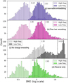 |
Fig. 3 Performance comparison for predicting IR spectra of 12 599 PAHs across charge states, evaluated using the EMD error (x-axis, log scale). NN models with two charge-encoding methods, learnable embedding (a) and one-hot encoding (b), are compared against two baselines: an identical NN without charge encoding (c) and a NN trained or tested only on neutral molecules (d). Vertical dashed lines indicate the mean EMD. |
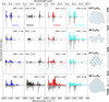 |
Fig. 4 Comparison of NN-predicted (positive y-axis) and DFT reference (mirrored) IR spectra for four PAHs chosen from different quartiles of the EMD error distribution. For each molecule, spectra are shown for the −1, 0, +1, and +2 charge states. |
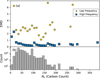 |
Fig. 5 (a) Averaged EMD error (dimensionless) vs. PAH size with a bin width of 10 in a five-fold cross-validation test using the NN with learnable embedding, (b) Size distribution of the PAHs in the training dataset. |
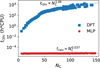 |
Fig. 6 Computational time for calculating IR spectra vs. PAH size (NC). Results compare the NN model (circles, sequential execution on Intel i7-13700 CPU) with DFT calculations at B3LYP/6-311+g level (squares, parallelized across 40 Intel Xeon E5-2680 CPU cores). |
3.3 Astrophysical implications
The primary astrophysical value of this ML framework is its ability to bypass the steep  scaling constraints of quantum chemistry, enabling the construction of extensive spectral databases that are otherwise computationally prohibitive. Interpreting JWST observations of AIBs relies on libraries like the PAHdb, yet large PAHs that were considered the primary AIB carriers (Sellgren 1984; Allamandola et al. 1989; Hanine et al. 2020; Meng & Wang 2023) constitute only small fraction of the database due to DFT costs. Our model overcomes this limitation by achieving orders-of-magnitude acceleration with near-constant inference cost, allowing high-throughput screening of species and enabling exploration of the vast chemical spaces represented in datasets like the computational database of polycyclic aromatic systems (COMPASS) (Wahab et al. 2022).
Second, characterizing the ionization state of interstellar PAHs is important for determining the physical conditions of the interstellar medium. While the community has traditionally relied on empirical band ratios (Gregg et al. 2026; Baron et al. 2025; Maragkoudakis et al. 2023), our RF classifier demonstrates that the complete IR emission profile can serve as a high-dimensional fingerprint, identifying charge states with over 99% accuracy. We identify specific diagnostic regions, such as the underappreciated cationic feature at 9.8 μm, that enhance the distinction between anionic, neutral, and cationic populations.
Finally, our analysis of a consistent dataset (3465 species) allows for a statistical reassessment of established astrophysical benchmarks. We find that anionic PAHs exhibit strong emissions in the 3.3 and 6.2 μm bands, traditionally attributed to neutrals and cations, and consistently match or exceed cation intensities across the 6–9 μm region. These results suggest a more prominent role for anionic PAHs in interstellar IR emission than previously recognized.
4 Conclusions
In conclusion, we have developed charge-aware NN models to predict the IR spectra of PAHs. Trained on a large dataset from DFT calculations and existing databases covering neutral, anionic, and cationic states, the primary model predicts normalized IR spectra with near-DFT accuracy. It achieves a computational speed-up of several orders of magnitude and robustly handles molecules with up to 150 carbon atoms. However, generalizability to very large PAHs (NC > 160) remains constrained by limited training data, a bottleneck inherent to traditional DFT methods. Future work that employs physics-informed ML approaches such as ML molecular dynamics (Mai et al. 2025) may help in overcoming this limitation. We also demonstrate that a simple RF classifier can accurately determine a PAH's charge state from its spectrum alone.
Besides the predictive models, our analysis of the DFT data reveals key deviations from prior spectral benchmarks. Anions exhibit the highest intensity in the 3.3 and 6.2 μm bands, which are traditionally attributed to neutrals and cations, respectively, while cations dominate at 11.2 μm. Moreover, across the 6.2, 7.7, 8.6, and 12.5–14.5 μm complexes, anions consistently match or exceed cation intensities. These findings suggest a more prominent role for anionic PAHs in the interstellar IR spectrum than previously recognized.
Data availability
The source code and data of the NN models are openly accessible at the Git repository: ChargeEncoding-IRPrediction.
Acknowledgements
The authors acknowledge financial support from the National Natural Science Foundation of China (Grant No. 12463005 and 11964002). This work was supported by the Guangxi Talent Programme (Highland of Innovation Talents).
References
- Allamandola, L. J., Tielens, A. G. G. M., & Barker, J. R. 1989, ApJS, 71, 733 [Google Scholar]
- Allamandola, L. J., Hudgins, D. M., & Sandford, S. A. 1999, ApJ, 511, L115 [Google Scholar]
- Andrews, H., Boersma, C., Werner, M. W., et al. 2015, ApJ, 807, 99 [NASA ADS] [CrossRef] [Google Scholar]
- Bakes, E. L. O., Tielens, A. G. G. M., & Bauschlicher, C. W. 2001, ApJ, 556, 501 [NASA ADS] [CrossRef] [Google Scholar]
- Baron, D., Sandstrom, K. M., Sutter, J., et al. 2025, ApJ, 978, 135 [Google Scholar]
- Bauschlicher, C. W., Jr., & Langhoff, S. R. 1997, Spectrochim. Acta A, 53, 1225 [Google Scholar]
- Bauschlicher, C. W., Jr., Peeters, E., & Allamandola, L. J. 2008, ApJ, 678, 316 [NASA ADS] [CrossRef] [Google Scholar]
- Bauschlicher, C. W., Jr., Peeters, E., & Allamandola, L. J. 2009, ApJ, 697, 311 [NASA ADS] [CrossRef] [Google Scholar]
- Bauschlicher, C. W., Jr., Ricca, A., Boersma, C., & Allamandola, L. J. 2018, ApJS, 234, 32 [NASA ADS] [CrossRef] [Google Scholar]
- Beglaryan, B. G., Zakuskin, A. S., Nemchenko, V. A., & Labutin, T. A. 2025, J. Chem. Inf. Model., 65, 4854 [Google Scholar]
- Boersma, C., Bauschlicher, C. W., Jr., Ricca, A., et al. 2014, ApJS, 211, 8 [NASA ADS] [CrossRef] [Google Scholar]
- Calvo, F., Simon, A., Parneix, P., Falvo, C., & Dubosq, C. 2021, J. Phys. Chem. A, 125, 5509 [Google Scholar]
- Draine, B. T., & Li, A. 2001, ApJ, 551, 807 [NASA ADS] [CrossRef] [Google Scholar]
- Draine, B. T., & Li, A. 2007, ApJ, 657, 810 [CrossRef] [Google Scholar]
- Eisenberg, D., & Shenhar, R. 2012, WIREs Comput. Mol. Sci., 2, 525 [Google Scholar]
- Frisch, M. J., Trucks, G. W., Schlegel, H. B., et al. 2016, Gaussian 16 Revision C.01 [Google Scholar]
- Gregg, B., Calzetti, D., Adamo, A., et al. 2026, ApJ, 997, 20 [Google Scholar]
- Hanine, M., Meng, Z., Lu, S., et al. 2020, ApJ, 900, 188 [NASA ADS] [CrossRef] [Google Scholar]
- Hony, S., Van Kerckhoven, C., Peeters, E., et al. 2001, A&A, 370, 1030 [CrossRef] [EDP Sciences] [Google Scholar]
- Hudgins, D. M., Bauschlicher, C. W., Jr., & Allamandola, L. J. 2001, Spectrochim. Acta A, 57, 907 [Google Scholar]
- Jahn, H. A., & Teller, E. 1937, Proc. R. Soc. Lond. A, 161, 220 [Google Scholar]
- Knuth, K. H. 2006, arXiv e-prints [arXiv:physics/0605197] [Google Scholar]
- Kovács, P., Zhu, X., Carrete, J., Madsen, G. K. H., & Wang, Z. 2020, ApJ, 902, 100 [CrossRef] [Google Scholar]
- Laurens, G., Rabary, M., Lam, J., Peláez, D., & Allouche, A.-R. 2021, Theor. Chem. Acc., 140, 66 [Google Scholar]
- Li, A. 2020, Nat. Astron., 4, 339 [CrossRef] [Google Scholar]
- Li, K., Li, A., Yang, X. J., & Fang, T. 2024, ApJ, 961, 107 [Google Scholar]
- Li, G., Ou, C., Wang, J., Zhang, Y., & Wang, Z. 2026, A&A, 707, A72 [NASA ADS] [CrossRef] [EDP Sciences] [Google Scholar]
- Liao, Q., Wang, J., Xie, P., Liang, E., & Wang, Z. 2023, RAA, 23, 122001 [Google Scholar]
- Lu, S., Meng, Z., Xie, P., Liang, E., & Wang, Z. 2021, A&A, 656, A84 [NASA ADS] [CrossRef] [EDP Sciences] [Google Scholar]
- Mai, X., Wang, Z., Pan, L., et al. 2025, MNRAS, 541, 3073 [Google Scholar]
- Maragkoudakis, A., Peeters, E., & Ricca, A. 2020, MNRAS, 494, 642 [NASA ADS] [CrossRef] [Google Scholar]
- Maragkoudakis, A., Peeters, E., Ricca, A., & Boersma, C. 2023, MNRAS, 524, 3429 [Google Scholar]
- Maragkoudakis, A., Boersma, C., Temi, P., et al. 2025, ApJ, 979, 90 [Google Scholar]
- Mattioda, A. L., Hudgins, D. M., Boersma, C., et al. 2020, ApJS, 251, 22 [NASA ADS] [CrossRef] [Google Scholar]
- McGill, C. J., Forsuelo, M., Guan, Y., & Green, W. H. 2021, J. Chem. Inf. Model., 61, 2594 [Google Scholar]
- Meng, Z., & Wang, Z. 2023, MNRAS, 526, 3335 [Google Scholar]
- Meng, Z., Zhu, X., Kovács, P., Liang, E., & Wang, Z. 2021, ApJ, 922, 101 [Google Scholar]
- Meng, Z., Zhang, Y., Liang, E., & Wang, Z. 2023, MNRAS, 525, L29 [NASA ADS] [CrossRef] [Google Scholar]
- Morgan, H. L. 1965, J. Chem. Doc., 5, 107 [Google Scholar]
- Peeters, E., Hony, S., van Kerckhoven, C., et al. 2002, A&A, 390, 1089 [NASA ADS] [CrossRef] [EDP Sciences] [Google Scholar]
- Peeters, E., Bauschlicher, C. W., Jr., Allamandola, L. J., et al. 2017, ApJ, 836, 198 [NASA ADS] [CrossRef] [Google Scholar]
- Peeters, E., Mackie, C., Candian, A., & Tielens, A. G. G. M. 2021, Acc. Chem. Res., 54, 1921 [Google Scholar]
- Ramakrishnan, R., Dral, P. O., Rupp, M., & von Lilienfeld, O. A. 2015, J. Chem. Theory Comput., 11, 2087 [Google Scholar]
- Ricca, A., Bauschlicher, C. W., Jr., Boersma, C., Tielens, A. G. G. M., & Allamandola, L. J. 2012, ApJ, 754, 75 [NASA ADS] [CrossRef] [Google Scholar]
- Ricca, A., Bauschlicher, C. W., Jr., Roser, J. E., & Peeters, E. 2018, ApJ, 854, 115 [Google Scholar]
- Ricca, A., Boersma, C., & Peeters, E. 2021, ApJ, 923, 202 [NASA ADS] [CrossRef] [Google Scholar]
- Ricca, A., Roser, J. E., Boersma, C., Peeters, E., & Maragkoudakis, A. 2024, ApJ, 968, 128 [Google Scholar]
- Ricca, A., Boersma, C., Maragkoudakis, A., et al. 2026, ApJS, 282, 7 [Google Scholar]
- Sellgren, K. 1984, ApJ, 277, 623 [Google Scholar]
- Shannon, M. J., Stock, D. J., & Peeters, E. 2016, ApJ, 824, 111 [NASA ADS] [CrossRef] [Google Scholar]
- Stephens, P. J., Devlin, F. J., Chabalowski, C. F., & Frisch, M. J. 1994, J. Phys. Chem., 98, 11623 [CrossRef] [Google Scholar]
- Stienstra, C. M. K., van Wieringen, T., Hebert, L., et al. 2025, J. Chem. Inf. Model., 65, 2385 [Google Scholar]
- Tang, G., He, J., Wang, Z., & Qiu, D. 2026, MNRAS, 546, 283 [Google Scholar]
- Tielens, A. G. G. M. 2008, ARA&A, 46, 289 [Google Scholar]
- van Diedenhoven, B., Peeters, E., van Kerckhoven, C., et al. 2004, ApJ, 611, 928 [NASA ADS] [CrossRef] [Google Scholar]
- Wahab, A., Pfuderer, L., Paenurk, E., & Gershoni-Poranne, R. 2022, J. Chem. Inf. Model., 62, 3704 [Google Scholar]
- Yang, X. J., Li, A., He, C. Y., & Glaser, R. 2021, ApJS, 255, 23 [NASA ADS] [CrossRef] [Google Scholar]
Appendix A Experimental validation of DFT calculations
To evaluate the accuracy of our computational framework, we benchmarked the DFT results against a representative subset of 84 PAHs with available laboratory spectra from the PAHdb. Figure A.1 presents ten illustrative comparisons, categorized into five intervals of prediction accuracy. These examples range from high-fidelity spectral matches to cases with more pronounced deviations. Overall, the benchmarking results confirm that our DFT-calculated spectra maintain strong consistency with experimental data across the sampled chemical space.
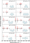 |
Fig. A.1 Comparison between DFT-calculated (positive y-axis) and experimental (mirrored negative y-axis) IR spectra for ten representative PAHs. Panels (a)–(j) are organized to reflect the full distribution of prediction errors observed across the 84-species benchmark set, from the highest-fidelity matches (a) to the largest deviations (j). All spectra are normalized to unit intensity for visual comparison. |
All Tables
Performance metrics and the top-five most important bands for charge-state prediction using the RF classifier.
Mean EMD (dimensionless) for predictions using absolute vs. relative intensities.
All Figures
|
Fig. 1 Distribution of carbon-atom counts (NC, in log scale) for PAHs in our generated dataset (orange bars) and for those selected from the PAHdb (green bars). The stacked segments within each bar represent different charge states. |
| In the text | |
|
Fig. 2 Statistical analysis of IR spectra for 3465 PAHs in neutral (black), cationic (red), and anionic (blue) states. (a) Mean spectra from 2.5 to 15 μm. Shaded regions highlight key AIBs. (b)–(g) Close-ups of major bands with peak positions marked. (h)-(m) Peak position vs. carbon atom count (NC). Points show binned averages, and error bars are standard deviations. |
| In the text | |
|
Fig. 3 Performance comparison for predicting IR spectra of 12 599 PAHs across charge states, evaluated using the EMD error (x-axis, log scale). NN models with two charge-encoding methods, learnable embedding (a) and one-hot encoding (b), are compared against two baselines: an identical NN without charge encoding (c) and a NN trained or tested only on neutral molecules (d). Vertical dashed lines indicate the mean EMD. |
| In the text | |
|
Fig. 4 Comparison of NN-predicted (positive y-axis) and DFT reference (mirrored) IR spectra for four PAHs chosen from different quartiles of the EMD error distribution. For each molecule, spectra are shown for the −1, 0, +1, and +2 charge states. |
| In the text | |
|
Fig. 5 (a) Averaged EMD error (dimensionless) vs. PAH size with a bin width of 10 in a five-fold cross-validation test using the NN with learnable embedding, (b) Size distribution of the PAHs in the training dataset. |
| In the text | |
|
Fig. 6 Computational time for calculating IR spectra vs. PAH size (NC). Results compare the NN model (circles, sequential execution on Intel i7-13700 CPU) with DFT calculations at B3LYP/6-311+g level (squares, parallelized across 40 Intel Xeon E5-2680 CPU cores). |
| In the text | |
|
Fig. A.1 Comparison between DFT-calculated (positive y-axis) and experimental (mirrored negative y-axis) IR spectra for ten representative PAHs. Panels (a)–(j) are organized to reflect the full distribution of prediction errors observed across the 84-species benchmark set, from the highest-fidelity matches (a) to the largest deviations (j). All spectra are normalized to unit intensity for visual comparison. |
| In the text | |
Current usage metrics show cumulative count of Article Views (full-text article views including HTML views, PDF and ePub downloads, according to the available data) and Abstracts Views on Vision4Press platform.
Data correspond to usage on the plateform after 2015. The current usage metrics is available 48-96 hours after online publication and is updated daily on week days.
Initial download of the metrics may take a while.