| Issue |
A&A
Volume 709, May 2026
|
|
|---|---|---|
| Article Number | A38 | |
| Number of page(s) | 12 | |
| Section | Interstellar and circumstellar matter | |
| DOI | https://doi.org/10.1051/0004-6361/202556975 | |
| Published online | 01 May 2026 | |
PDRs4All
XIX. The evolution of the PAH ionisation and PAH size distribution across the Orion Bar
1
NASA Ames Research Center,
MS 245-6, Moffett Field, CA
940351000,
USA
2
Department of Physics & Astronomy, The University of Western Ontario,
London, ON N6A 3K7,
Canada
3
Institute for Earth and Space Exploration, The University of Western Ontario,
London, ON N6A 3K7,
Canada
4
Carl Sagan Center, SETI Institute,
339 Bernardo Avenue, Suite 200, Mountain View, CA
94043,
USA
5
Department of Astronomy, University of Michigan,
1085 South University Avenue, Ann Arbor, MI
48109,
USA
6
Institut de Recherche en Astrophysique et Planétologie, Université Toulouse III – Paul Sabatier,
CNRS, CNES, 9 Av. du colonel Roche, 31028 Toulouse Cedex 04,
France
7
School of Physics, University of Hyderabad,
Hyderabad, Telangana
500046,
India
8
Faculty of Computer Science & Technology, Algoma University,
Sault Ste. Marie, ON P6A 2G4,
Canada
9
Institut d’Astrophysique Spatiale, Université Paris-Saclay,
CNRS, Bâtiment 121, 91405 Orsay Cedex,
France
10
Instituto de Física Fundamental (CSIC),
Calle Serrano 121-123,
28006
Madrid,
Spain
11
IPAC, California Institute of Technology,
Pasadena, CA,
USA
12
Department of Astronomy, Graduate School of Science, The University of Tokyo,
7-3-1 Bunkyo-ku, Tokyo
113-0033,
Japan
13
Astronomy Department, University of Maryland,
College Park, MD
20742,
USA
14
Space Telescope Science Institute,
3700 San Martin Drive, Baltimore, MD
21218,
USA
15
School of Physics and Astronomy, Sun Yat-sen University,
2 Da Xue Road, Tangjia, Zhuhai
519000,
Guangdong Province,
China
★ Corresponding author: This email address is being protected from spambots. You need JavaScript enabled to view it.
Received:
25
August
2025
Accepted:
29
January
2026
Abstract
Context. JWST observations of the Orion Bar have revealed rich and diverse polycyclic aromatic hydrocarbon (PAH) emission. These observations allow for the first time a comprehensive characterisation of the charge state and size of the PAH population on morphologically resolved photodissociation regions (PDR) scales, properties closely linked to physical conditions of their inhabiting environments.
Aims. We investigate the evolution of the PAH population’s charge state and size across key physical zones in the Orion Bar, which include the H ii region, the atomic PDR (APDR), and three bright H I/H2 dissociation fronts (DF1, DF2, and DF3). We connect changes in the PAH charge and size as probed by empirical emission proxies with the varying physical properties of their surrounding environments.
Methods. Utilising the NASA Ames PAH Infrared Spectroscopic Database (PAHdb) and the pyPAHdb spectral modelling tool, we analysed the MIRI-MRS observations of the Orion Bar from the ‘PDRs4All’ JWST Early Release Science Program. Decomposition and modelling were performed on the 5−15 μm spectrum across the entire JWST mosaic, as well as on the weighted average spectra of the five key physical zones.
Results. pyPAHdb modelling reveals the fractional contribution of the different PAH charge states and sizes to the total PAH emission across the Orion Bar. Cationic PAH emission peaks in the APDR region, where neutral PAHs make a minimal contribution. Emission from neutral PAHs peaks in the H ii region that consists of emission from a face-on PDR associated with the background OMC-1 molecular cloud, and in the molecular cloud regions past DF2. The PAH anions are observed deep within the DF2 and DF3 zones. Small and medium-sized PAHs make up ∼ 70% of the PAH emission across the mosaic, with the peak of the small PAH emission found between the DF2 and DF3 zones. The average PAH size in the Orion Bar ranges between ∼ 60−74 NC. The modelling reveals regions of top-down PAH formation at the ionisation front, and bottom-up PAH formation within the molecular cloud region. The PAH ionisation parameter, γ, ranges between ∼ 2−9 × 10⁴. Intensity ratios that are empirical tracers of PAH ionisation (I6.2/I11.2, I7.7/I11.2, I8.6/I11.2) scale well with γ in regions encompassing edge-on or face-on PDR emission, but their correlation weakens within the molecular cloud zone.
Conclusions. Modelling of the 5−15 μm PAH spectrum with pyPAHdb achieves a comprehensive characterisation of the net contribution of neutral and cationic PAHs across different environments, whereas empirical PAH proxy intensity ratio tracers can be highly variable and unreliable outside regions dominated by PDR emission. The derived average PAH size in the different physical zones is consistent with a view of PAHs being more extensively subjected to ultraviolet processing closer to the ionisation front, and less affected within the molecular cloud.
Key words: techniques: spectroscopic / HII regions / photon-dominated region (PDR) / infrared: ISM / planetary nebulae: individual: Orion Bar
© The Authors 2026
 Open Access article, published by EDP Sciences, under the terms of the Creative Commons Attribution License (https://creativecommons.org/licenses/by/4.0), which permits unrestricted use, distribution, and reproduction in any medium, provided the original work is properly cited.
This article is published in open access under the Subscribe to Open model. This email address is being protected from spambots. You need JavaScript enabled to view it. to support open access publication.
1 Introduction
A set of prominent emission features at 3.3, 6.2, 7.7, 8.6, 11.2, 12.7, 16.4, and 17.4 μm, with weaker features at surrounding wavelengths, are common to the infrared (IR) spectra of numerous astronomical sources. This emission from the so-called aromatic infrared bands (AIBs) is generally attributed to the family of polycyclic aromatic hydrocarbons (PAHs) and are due to vibrational emission of the carbon-carbon and carbon-hydrogen (C−H) bonds in the PAH molecules that become excited upon the absorption of far-ultraviolet (FUV; 6–13.6 eV) photons (Leger & Puget 1984; Allamandola et al. 1985). The PAH emission has been detected in the spectra of Milky Way sources, including planetary and reflection nebulae (e.g. Bregman et al. 1989; Beintema et al. 1996; Peeters et al. 2002a; Werner et al. 2004), protoplanetary discs (e.g. Vicente et al. 2013), H ii regions (e.g. Bregman et al. 1989; Peeters et al. 2002b), and a wide variety of galaxies and galactic nuclei (e.g. Hony et al. 2001; Peeters et al. 2004; Smith et al. 2007; Galliano et al. 2008; Sandstrom et al. 2012; Boersma et al. 2018; Maragkoudakis et al. 2018; Zang et al. 2022; Lai et al. 2022, 2023; García-Bernete et al. 2022; Maragkoudakis et al. 2022; Chastenet et al. 2023; Egorov et al. 2023; Rigopoulou et al. 2024; Maragkoudakis et al. 2025).
The PAH emission can offer unique insights into the local physical conditions of their host environments (e.g. Galliano et al. 2008; Boersma et al. 2015; Pilleri et al. 2015; Stock & Peeters 2017; Peeters et al. 2017; Maragkoudakis et al. 2022). For instance, the intensity of the UV radiation field, G0, in terms of the Habing field (Habing 1968) can be assessed through the empirical calibration of the I6.2/I11.2 PAH band ratio and the ionisation parameter γ ∝ G0 T1/2/ne, where T is the gas temperature and ne is the electron density (e.g. Galliano et al. 2008; Maragkoudakis et al. 2022). The unparalleled spatial resolution and sensitivity of JWST now allow for the calibration of these diagnostic tracers on spatially resolved scales within astronomical sources.
The study of PAH emission in photo-dissociation regions (PDRs) is of particular interest, as it encompasses emission from zones with different physical conditions and chemical stratification. The PDRs are the interfaces between molecular gas and the surrounding galactic medium, illuminated by FUV photons (6 eVE < 13.6 eV) from young massive stars. The Orion Bar is a prototypical strongly UV-irradiated PDR in the Orion Nebula (M42). Due to its nearly edge-on view and very high surface brightness, the Orion Bar is one of the most extensively studied sources (Tielens et al. 1993; Hogerheijde et al. 1995; Kassis et al. 2006; Goicoechea et al. 2016) and an excellent candidate to examine the evolution of PAH emission, the characteristics of its carriers, and their connection to the local physical conditions across the PDR.
In this work, we characterise the fractional contribution of the different PAH charge states and sizes to the total PAH emission by performing modelling of the 5−15 μm PAH emission spectrum across the Orion Bar’s JWST MIRI-MRS mosaic. This paper is structured as follows. Section 2 describes the observations, data reduction, and measurement of the PAH emission bands. Section 3 presents the analysis and results. A discussion and summary of our conclusions are given in Sections 4 and 5, respectively.
2 Observations and analysis
2.1 Anatomy of the Orion Bar
PDRs are mostly neutral regions in the interstellar medium (ISM) in which the physics and chemistry are regulated by FUV photons from nearby massive stars. Four characteristic zones are typically identified across PDRs: the ionisation front (IF) where the gas converts from fully ionised to fully neutral, the atomic PDR (APDR) where hydrogen exists primarily in atomic form, the H2 dissociation front (DF) where molecular hydrogen dissociates due to FUV radiation, and the molecular zone where the gas is nearly fully molecular.
The nearly edge-on geometry of Orion Bar’s PDR permits spatially resolved observations of the different (neutral atomic, and molecular) layers across the IF and DFs (see Peeters et al. 2024, their Fig. 14). Strong UV radiation from θ1 Ori C, the most massive and brightest star in the Trapezium cluster, powers and shapes the H ii region in the Orion Nebula. The IF, located at a physical distance of 0.27 pc from θ1 Ori C, separates the edge of the PDR from the surrounding H ii region. Beyond the IF, the first layers of the PDR are predominantly neutral and atomic, the so-called APDR zone. At ∼ 0.03 pc from the IF the FUV photon flux is sufficiently attenuated that most of the hydrogen becomes molecular, marking the beginning of the molecular PDR. Three such successive H2 ridges representing three edge-on DFs (DF1, DF2, and DF3) are located at increasing distances from the IF. We note that emission from PAHs and other PDR tracers (H2, CO, CH+, [OI] 63 and 145 μm, and [CII] 158 μm) in the H ii region originates from the background face-on PDR in OMC-1 (e.g. Bernard-Salas et al. 2012; Parikka et al. 2018; Goicoechea et al. 2019; Knight et al. 2022; Habart et al. 2024; Peeters et al. 2024). Beyond DF3 (BDF3), the emission suggests another layer of foreground or background PDR emission. Detection of [CI] 609 μm emission component at velocities different from the Bar (see Fig. 5 of Goicoechea et al. 2025) indicates a translucent component in the foreground or background of the Bar. However, Goicoechea et al. (2025) did not detect significant C2H hydrocarbon emission from the background OMC-1 gas. Hence, additional observations are required to characterise the nature of this region. Two proto-planetary discs are also present within the APDR zone, the proplyds 203–504 and 203–506 (Bally et al. 2000; Berné et al. 2023, 2024), although they are not embedded in the PDR but rather located in the line of sight toward the Bar (e.g. Haworth et al. 2023). Here, we focus on the characterisation of the PAH emission across the different zones in the Orion’s Bar PDR, i.e. the H ii region, the APDR, and the three DFs and their surroundings.
2.2 Observations and data reduction
The JWST Early Release Science (ERS) programme PDRs4All1 (Radiative feedback from massive stars, ID1288; Berné et al. 2022b) has obtained NIRCam and MIRI imaging (Habart et al. 2024) as well as NIRSpec and MIRI-MRS spectral mapping mode observations (Peeters et al. 2024; Chown et al. 2024; Van De Putte et al. 2024) of the Orion Nebula. The integral field unit (IFU) observations cover a 9 × 1 tiles mosaic, positioned to achieve an overlap between the NIRSpec and MIRI-MRS channel 1 fields of view (FoVs). From the assembled spectral cubes, a set of five template spectra have been extracted from apertures selected to be representative of the five key physical zones of the Orion Bar: the H ii region, the APDR, and the three bright H I/H2 DFs (DF1, DF2, and DF3) corresponding to three molecular hydrogen (H2) filaments, as identified in the NIRSpec FoV (Peeters et al. 2024).
In this work, we focus on the MIRI-MRS observations, utilising the first three MRS channels and all three sub-bands within each channel (short, medium, and long), which provide coverage of the main PAH bands, i.e. at 6.2, 7.7, 8.6, and 11.2 μm. We performed spectral decomposition and subsequent modelling of the PAH emission spectrum across the entire mosaic, as well as on the weighted average (template) spectra of the five key physical zones. The PAH emission spectrum modelling was performed using the NASA Ames PAH Infrared Spectroscopic Database2 (PAHdb; Bauschlicher et al. 2010; Boersma et al. 2014; Bauschlicher et al. 2018; Mattioda et al. 2020, Ricca et al. in prep.), which consists of the largest collection of quantumchemically computed absorption spectra of PAHs of various structures, charge states, sizes, and compositions, accompanied by a suite of modelling tools3.
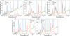 |
Fig. 1 Spectral decomposition of the five Orion Bar template spectra in the 5−15 μm wavelength region. The template spectra are shown in blue, the spectrum after the emission lines removal is shown in orange, the fitted baseline in green, and the resulting isolated PAH emission spectrum in red. |
2.3 Spectral decomposition
Isolation of the PAH emission component requires removal of the emission lines present in the spectrum (e.g. H i recombination lines, ro-vibrational and pure rotational H2 lines, and forbidden atomic lines; see Peeters et al. 2024 and Van De Putte et al. 2025) and the underlying continuum. We achieved this in two steps using the pybaseline4 library of algorithms. In the first step, the morphological algorithm was used to create the modelling curve. This performed a morphological opening transformation on the data and then selected the element-wise minimum between the opening and the average of a morphological erosion and dilation of the opening. The ‘half-window’ parameter defines the size of the window used for the morphological operators, allowing for the capture of only broad emission features, i.e. the PAH bands, excluding all the narrow emission lines in the spectrum (Figure 1, orange lines). In the second step, a baseline was fitted and subtracted from the resulting spectrum in step one, using the imodpoly (Improved Modified Polynomial) algorithm (Figure 1, green lines), which uses thresholding to iteratively fit a polynomial baseline to data. After the baseline subtraction, the pure PAH emission spectrum was obtained (Figure 1, red lines). Additionally, this process allows one to obtain the emission line spectrum by subtracting both the baseline and the PAH spectrum from the input observational spectrum. We note that no correction for extinction was applied to the spectra. Because the Orion Bar spectra do not exhibit strong absorption features (e.g. silicate absorption or ice features), pybaseline is well suited for extracting the underlying continuum. The spectral decomposition was performed on the entire MIRI-MRS mosaic and the five template spectra.
2.4 pyPAHdb modelling
The modelling of the PAH emission spectra was performed with the pyPAHdb5 tool. pyPAHdb was developed as one of the science-enabling products for the PDRs4All programme and is a streamlined version of the broader AmesPAHdbPythonSuite6 package from the PAHdb suite of tools. A first description of pyPAHdb was given in Shannon & Boersma (2018). pyPAHdb is designed to quickly and conveniently fit the PAH emission component of a (JWST) spectrum and break it down in terms of PAH charge and size, whereas the AmesPAHdbPythonSuite allows for more flexibility in the modelling parameters and the selection of the pool of PAHs. pyPAHdb streamlines the database-fitting by using a pre-computed matrix of highly over-sampled synthesised PAH emission spectra, under a specific modelling configuration. In the latest version of pyPAHdb the matrix is built from version 4.00- α of the library of computed spectra (Maragkoudakis et al. 2025), using pure PAH molecules of different charge states (neutral, cation, and anion PAHs) and sizes (20<NC<384). The emission spectrum was calculated utilising the ‘cascade’ emission model using an excitation energy of 7 eV, and each transition was convolved with a Gaussian emission profile with a full width at half maximum of 15.0 cm−17. Given that PAHs absorb an average photon energy of 8.1 eV at the IF (Knight et al. 2021) and the average absorbed photon energy decreases as the radiation field is attenuated as we progress into the PDR, we adopted an average photon energy of 7 eV for our analysis.
pyPAHdb returns the breakdown of the contributing PAHs in the fit in terms of the PAH charge and size. Specifically, the PAH charge breakdown provides the fractional contribution of the neutral, cationic, and anionic PAHs to the total PAH emission, while the PAH size breakdown provides the fractional contribution of the small (NC ≤ 50), medium (50<NC ≤ 70), and large (NC>70) PAHs in the fit. pyPAHdb has been especially geared to work with spectral mosaics and, as such, it also delivers maps of the cation-to-neutral fractions and the weighted average NC from the fitting weights of the contributing PAHs in the fit.
Modelling with pyPAHdb was performed on both the entire MIRI-MRS mosaic and the template spectra of the five key physical zones of the PDR. Figure 2 shows an example of the PAH charge and size breakdown of the APDR and DF3 template regions, and plots of the remaining regions are presented in Appendix B (Figure B.1). The figure demonstrates the high level of detail that the modelling is able to reproduce (see also Maragkoudakis et al. 2025), and reiterates the effect of charge on a PAH’s spectrum whereby the bulk of the intensity shifts from the 11–14 to the 6–9 μm region upon ionisation (Allamandola et al. 1999). Figures 3 and 4 present the different maps of the PAH charge breakdown and the PAH size, respectively. The maps of the PAH ionisation parameter (γ; see Section 3.2) and weighted average NC are shown in Figures 5 and 6, respectively. The map of the modelling error (σpyPAHdb) is presented in Appendix A (Figure A.1), which is typically between 10−15%. All results need to be considered within the limits of the employed (pyPAHdb) modelling and its sensitivity to parameter choices. Such aspects (e.g. different excitation energies, emission models, line profiles, and PAHdb library versions) have been thoroughly explored previously, in for example Andrews et al. (2015) and Maragkoudakis et al. (2025), and provide confidence in the overall approach.
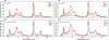 |
Fig. 2 PAH size (top sub-panels) and charge breakdown (bottom sub-panels) for the spectral templates of the APDR (left) and DF3 (right). Observations are shown in black and the total fit in red, and the separate breakdown components are given in the legend of each panel. |
2.5 PAH band measurements
Measurement of the PAH band strengths was performed on the pure PAH emission spectra by integrating the flux within defined wavelength intervals. The wavelength regions were determined by visual inspection after overplotting the PAH emission spectra of the five key physical regions (Figure 7). This method, while not necessarily as precise as a multi-component decomposition (e.g. Van De Putte et al. 2025; Khan et al. 2025a), has the advantage of capturing the bulk of the PAH emission, providing a good estimate of the PAH band intensity ratios efficiently for the ∼8 500 pixels that span the entire mosaic. Figure 8 presents the PAH intensity maps of the I6.2, I7.7, I8.6, and I11.2 μm bands, and Figure 9 the maps of the I6.2/I11.2, I7.7/I11.2, and I8.6/I11.2, PAH band intensity ratios. We have also obtained the I3.3 and I3.3/I11.2 maps from Schefter et al., (in prep.).
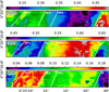 |
Fig. 3 PAH charge breakdown maps. The map of neutral PAHs is shown in the top panel, the PAH cations map in the middle panel, and the PAH anions map in the bottom panel. The colour bar shows the respective charge fractions, and for each map the range is scaled between the 0.5% and 99.5% percentiles. The colour map has been chosen to emphasise structure. |
3 Results
3.1 PAH charge and size across the Orion Bar
Figure 3 presents the maps of the PAH charge breakdown, i.e. the fractional contribution of the neutral (fneut), cation (fcat), and anion (fan) PAHs to the total PAH emission. It is clear from Figure 3 that the dominant charge state changes across the FoV, with neutral PAHs dominating in the line of sight towards the H ii region, cationic PAHs in the APDR, and anionic PAHs in the molecular PDR. The PAH emission in the line of sight towards the H ii region is actually originating from the background face-on PDR in OMC-1 (e.g. Peeters et al. 2024). In this region, approximately 40%−55% of the total PAH emission is due to neutral PAHs, ∼ 45%−60% due to PAH cations, and ∼ 5% due to PAH anions. The PAH emission in the APDR is dominated by cations (60%−70%), followed by neutrals (25%), and then anions (10%−15%). Moving towards DF1, and into DF2 and DF3 zones, where the flux of FUV photons is significantly attenuated (Peeters et al. 2024; Habart et al. 2024), fneut increases progressively from 25% to 40%, while fcat decreases from 60% to 45%, and fan makes its maximum contribution (up to 20%) in the DF3 region. In the region beyond DF3, fneut is ∼ 30−40%, fcat is ∼ 50−65%, and fan reaches up to ∼ 20%. The peak of PAH anion emission is observed deep within the DF2 and DF3 zones. As the FUV radiation is more attenuated deeper into the PDR, a change in the charge balance is expected, such as an increase in neutral and anionic PAHs (Bakes & Tielens 1994), although anions are expected to be present deeper within the molecular cloud.
The PAH size breakdown maps (Figure 4) present the fractional contribution of small (fsmall), medium (fmed), and large (flarge) PAHs to the total PAH emission, revealing regions where the different PAH size classes have a prevalent contribution. Large PAHs (NC > 70) contribute overall between ∼ 20−40%, with the highest flarge found in the H ii region close to the IF, between DF1 and DF3, and beyond DF3. Medium-sized PAHs (50<NC ≤ 70) contribute ∼ 10−50% to the total PAH emission. 40−50% of fmed is found in the H ii region and the APDR region closest to the IF, while the lowest contribution (∼ 20−25%) is between DF2 and DF3. The smaller PAHs (NC ≤ 50) make a ∼ 25−50% contribution to the total PAH emission. The highest fsmall(45−50%) is observed between DF2 and DF3, deep within the molecular cloud where small PAHs are less prone to photodissociation, and the lowest contribution (25−30%) is seen in the H ii region.
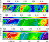 |
Fig. 4 PAH size breakdown maps. The map of large PAHs (NC<70) is shown in the top panel, the medium-sized PAHs (50<NC ≤ 70) map in the middle panel, and the small PAHs (NC ≤ 50) in the bottom panel. The colour bar shows the respective size fractions, and for each map the range is scaled between the 0.5% and 99.5% percentiles. |
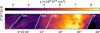 |
Fig. 5 Map of the PAH ionisation parameter (γ) obtained from the pyPAHdb modelling. White lines indicate the IF and the three DFs. |
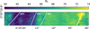 |
Fig. 6 Map of the average NC obtained from pyPAHdb modelling. White lines indicate the IF and the three DFs. |
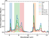 |
Fig. 7 Wavelength regions adopted for the measurement of the different PAH emission intensities, as deduced from the five spectral templates. The wavelength intervals are defined as follows: PAH6.2 μm: 6.0−6.6 μm; PAH7.7 μm: 7.0−8.2 μm; PAH8.6 μm: 8.2−9.15 μm; and PAH11.2 μm: 11.1− 11.7 μm. |
3.2 The PAH ionisation parameter (γ)
The ionisation parameter, γ, provides a description of the PAH ionisation balance as a function of local physical parameters, in particular the intensity of the radiation field (G0), the gas temperature (Tgas), and the electron density (ne). When assuming two accessible ionisation states and parameters applicable for circumcoronene (C54 H12), which is considered representative of an average interstellar PAH (NC=50−100; Croiset et al. 2016), the PAH ionisation parameter can be expressed as
![Mathematical equation: $\gamma \equiv\left(G_{0} \times \sqrt{T_{\mathrm{gas}}}\right)/n_{\mathrm{e}}=2.66\left(\frac{n_{\mathrm{PAH}^{+}}}{n_{\mathrm{PAH}^{0}}}\right)\left[\times 10^{4} \mathrm{~K}^{1/2} \mathrm{~cm}^{3}\right],$](/articles/aa/full_html/2026/05/aa56975-25/aa56975-25-eq1.png) (1)
where nPAH+ and nPAH0 are the PAH cation and neutral densities, which correspond to fcat and fneut, respectively, as determined from the pyPAHdb modelling (Tielens 2005; Boersma et al. 2014).
(1)
where nPAH+ and nPAH0 are the PAH cation and neutral densities, which correspond to fcat and fneut, respectively, as determined from the pyPAHdb modelling (Tielens 2005; Boersma et al. 2014).
Figure 5 presents the map of γ. Values are ranging between 2- 9 × 10⁴ K1/2 cm3. γ peaks in the APDR region between the IF and DF1 (6−8.5 × 10⁴ K1/2 cm3), where fcat is the highest and fneut lowest (Figures 3 4). Between DF1 and DF2, γ is ∼ 5 × 10⁴ K1/2 cm3, dropping to ∼ 4 × 10⁴ K1/2 cm3 beyond DF2, and has the lowest value (∼ 3 × 10⁴ K1/2 cm3) in the zone from the IF towards θ1 Ori C, which consists of emission originating from the background face-on PDR.
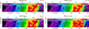 |
Fig. 8 Maps of the 6.2 μm 7.7 μm, 8.6 μm, and 11.2 μm PAH flux (in erg s−1 cm−2). The rectangular apertures of the five template regions are indicated, along with lines for the IF and DFs. |
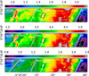 |
Fig. 9 PAH band intensity ratio maps. The rectangular apertures of the five template regions are indicated, along lines for the IF and DFs. |
3.3 The average PAH size
Figure 6 presents the map of the average PAH size in terms of  weighted by their emission contribution to the total emission.
  ranges between 60 and 74 C atoms. It peaks at the IF where small PAHs are less present due to photodissociation (see also Figure 4, bottom panel). From the IF and up to DF2 the
  is ∼ 70 C atoms, and drops to ∼ 62 C atoms in the molecular hydrogen region between DF2 and DF3. In the region beyond DF3 and in the H ii zone, the
  is ∼ 66−470 C atoms.
3.4 Modelling of the five key physical zone spectra
Five key regions have been identified in the NIRSpec (Peeters et al. 2024) and NIRCam (Habart et al. 2024) observations, representative of the key physical zones of the Orion Bar mosaic: the H ii region, the APDR, and three bright H I/H2 DFs (see Figure 8). Here, we perform pyPAHdb modelling of the five MIRI-MRS template spectra (Chown et al. 2024), which are the flux-weighted average of the pixels in the extraction apertures described in Peeters et al. (2024). Table 1 presents derived parameters for the five template spectra, and parameter values of the regions between the key physical zones denoted by the IF and DFs (H ii-IF, APDR-DF1, DF1-DF2, DF2-DF3, and DF3-BDF3). The PAH charge and size breakdowns, including the derivative γ and  parameters, are in agreement with the ranges of the broader and surrounding regions in the mosaic (Sections 3.1–3.3 and Table 1) in which the five regions reside.
3.5 PAH band strengths and relative intensities
Empirical calibrations involving the intensities of PAH emission bands sensitive to charge and size have been used to trace the charge state and size distribution of PAHs within and among astronomical sources. Such calibrations can be determined from models with assumptions on the PAH size distribution, the stochastic heating of PAHs, the absorption efficiencies, and so on (e.g. Schutte et al. 1993; Draine & Li 2007; Galliano et al. 2008; Stock et al. 2016; Draine et al. 2021), or derived without such assumptions from the ground up, from quantum-chemically computed spectra of PAH populations with various charge states and sizes (e.g. Cami 2011; Ricca et al. 2012; Boersma et al. 2013, 2015; Andrews et al. 2015; Boersma et al. 2018; Croiset et al. 2016; Maragkoudakis et al. 2020, 2023a,b).
To examine the relation of pyPAHdb-derived parameters (γ,  ) with the PAH intensity ratios employed in empirical calibrations, we have measured the integrated specific surface brightnesses (‘surface brightnesses’ hereafter) of the main PAH bands at 6.2, 7.7, 8.6, and 11.2 μm (Section 2.5), and generated their intensity maps, shown in Figure 8. We note that the wavelength region used to measure the I8.6 may include contribution from weaker features at 8.223 and 8.330 μm (Chown et al. 2024), which can be more prominent in the APDR region (Figure 7). These maps were then used to construct I6.2/I11.2, I7.7/I11.2, and I8.6/I11.2 PAH intensity ratio maps (Figure 9).
The surface brightness of all the PAH bands peaks within the APDR zone (Peeters et al. 2024; Habart et al. 2024; Pasquini et al. 2024; Khan et al. 2025a, Schefter et al., in prep.; Khan et al. 2025b), between the IF and DF1, gradually decreasing towards the molecular cloud region. Despite this gradual drop in surface brightness, all bands have relatively elevated values on the DF3 boundary compared to its immediate surrounding regions. Regions of weaker emission are found in the H ii zone and beyond DF3. The surface brightness in these regions decreases compared to the APDR by a factor of ∼ 10 in the case of the I6.2 and I8.6 surface brightness, and by a factor of ∼ 5−6 for the I7.7 and I11.2 surface brightness. Similar trends are observed in the I6.2/I11.2, I7.7/I11.2, I8.6/I11.2 PAH surface brightness ratio maps (Figure 9). The PAH surface brightness ratios peak within the APDR zone, while regions with lower values are in zones beyond DF3 and in the H ii region.
pyPAHdb derived parameters for the five template spectra (H ii APDR, DF 1, DF 2, and DF 3) and average parameter values of the regions between the key physical zones (H ii-IF, APDR-DF1, DF1-DF2, DF2-DF3, and DF3-BDF3).
3.6 γ-PAH intensity ratio calibrations
The pyPAHdb-determined ionisation parameter, γ, is compared against empirical tracers of PAH ionisation, i.e. the I6.2/I11.2, I7.7/I11.2, and I8.6/I11.2 relative PAH band intensity ratios (Figure 10). A linear relation between γ and the empirical tracers is observed for the majority of regions (pixels) across the mosaic. Colour-coding of the γ-PAH intensity ratio correlation as a function of the distance from the edge of the mosaic, indicative of the distance from θ1 Ori C, reveals a dependence of this correlation on distance, i.e. within the different physical regions. The bottom panels of Figure 10 show the correlation for the individual pixels of each template region.
The H II and APDR regions span a wide range in γ and PAH intensity ratios, with both quantities increasing from the H II zone towards and across the APDR. Both regions present similar γ−I6.2/I11.2 and γ−I7.7/I11.2 correlations (γ−I6.2,7.7/I11.2). Pixels located in the region between the IF and DF1, but outside the APDR template, form a distinctive sequence from the H ii and APDR template regions (Figure 10, bottom panels). Specifically, the γ−I6.2,7.7/I11.2 relations in the regions following the APDR and towards the DFs, including DF1, have a shallower slope from the corresponding correlations in the APDR–H ii regions, with γ and the I6.2,7.7/I11.2 ratios decreasing with the distance from the Bar. These regions maintain linear correlations among γ–I6.2, 7.7/I11.2, offset from the APDR–H ii template sequence, and with a somewhat larger scatter in the γ−I7.7/I11.2 case. The correlations of the regions starting from the edge of the mosaic (towards θ1 Ori C) and up to the DF1 are less separated in the γ−I8.6/I11.2 case, although with more scatter compared to the γ−I6.2,7.7/I11.2 correlations.
Moving from DF1 towards the DF2 and DF3 regions, the correlations between γ and the PAH ionisation proxies (IX/I11.2) begin to break. However, the pixels in the regions beyond DF3 (dark red pixels in Figure 10) exhibit a linear γ−IX/I11.2 correlation, albeit with a large scatter. In the γ−I6.2,7.7/I11.2 case, those pixels have a similar correlation with the pixels between the IF and DF1, excluding the APDR template region, while in the γ–I8.6/I11.2 case they appear in line with the correlation for the H II to DF1 pixels.
3.7 The NC−I3.3/I11.2 relation
The average number of carbon atoms NC retrieved from the pyPAHdb modelling of the 5−15 μm observations is compared against the well-defined I3.3/I11.2 empirical tracer for PAH size (e.g. Schutte et al. 1993; Ricca et al. 2012; Croiset et al. 2016; Maragkoudakis et al. 2020; Knight et al. 2021; Maragkoudakis et al. 2023a,b). For the comparison, we incorporate the PAH 3.3 μm measurements from Schefter et al. (in prep.) and show the I3.3/I11.2− correlation for the five key physical zones (Figure 11) along with contours for pixels within three standard deviations from the mean in each template region. Moving from the DF3 region towards the APDR, the relative I3.3/I11.2 PAH intensity gradually decreases (Schefter et al., in prep.), which follows an increase in
  (Figure 6). Towards the IF, smaller PAHs become more prone to photodissociation, resulting in a decrease in the I3.3 intensity and an increase in
  , as intermediate to large PAHs become more abundant (Figure 4). The H II region, where PAH emission originates from the background face-on PDR, diverges from the observed correlation. While the H II region contours of the 3 σ pixels overlap with the DF1 and APDR contours, the average I3.3/I11.2 value of the H II template is lower, driven by outliers outside the 3 σ cut-off. The unique behaviour of PAH emission in the H II region has been previously noted (Khan et al. 2025a) and may be attributed to geometric effects or differences in the characteristics of the UV field at the IF (Peeters et al. 2024).
The observed I3.3/I11.2− correlation is the product of the intrinsic response of different-sized PAHs to the UV field, where larger PAHs are contributing most of their emission at longer wavelengths and smaller PAHs are contributing predominantly to the emission at shorter wavelengths (Allamandola et al. 1989; Schutte et al. 1993). Therefore, PAH bands with large wavelength separation and of the same charge state (neutral) can effectively trace the different ends of the PAH size distribution, and can therefore describe
  . The I3.3/I11.2 ratio is a particularly good tracker of PAH size because both bands are due to CH stretches and arise primarily from neutral PAHs. Using the Maragkoudakis et al. (2020) PAH charge–size grid, we can obtain a fitting-independent description of the size distribution of PAHs in the five template regions (Figure 12). The
  of the template regions gradually increases moving from the DF3 to the H II region, as the I11.2/I3.3 ratio increases (I3.3/I11.2 decreases). The
  values were calculated as the average NC recovered from the ‘25% Neutral + 75% Cation’ and ‘Cation’ tracks of the charge-size grid (Maragkoudakis et al. 2020, their Eq. (3)) in which the template regions reside. Specifically, the
  values for the five template regions are H II:
  =67, APDR:
  =64, DF 1:
  =62, DF 2:
  =55, DF 3:
  =50. The
  recovered from pyPAHdb modelling, in the absence of the 3.3 μm PAH band, shows similar scaling with the I3.3/I11.2, i.e. increasing with decreasing I3.3/I11.2, as in the charge–size grid (apart from the H ii region; see previous paragraph). The
  values returned from pyPAHdb (Table 1 and Figure 11) and those from observational PAH ratio proxies (I3.3/I11.2) in conjunction with PAHdb models (e.g. Maragkoudakis et al. 2020, 2023a,b) are expected to show differences, given the additional information on the small end of the PAH size distribution obtained from the 3.3 μm band intensity in the latter case and fundamentally using different sets of PAH spectra for both modelling approaches. In addition, extinction may affect the measured I11.2/I3.3 intensity ratio, with extinction-corrected values potentially shifting the deduced
  to lower values in the charge-size diagram. Nevertheless, a comparison of the
  recovered by pyPAHdb between different regions provides a consistent description of the size variation in PAHs among these regions (Figures 11 and 12).
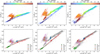 |
Fig. 10 Correlations between the different empirical PAH ionisation proxies (I6.2/I11.2, left panels; I7.7/I11.2, middle panels; I8.6/I11.2, right panels) and the PAH ionisation parameter (γ) deduced from pyPAHdb modelling. In the top panels, the pixels are colour-coded based on their vertical distance from the edge of the mosaic, which is indicative of the projected distance from θ1 Ori C. In the bottom panels, pixels corresponding to each of the five key physical regions are assigned a specific colour (H ii in green, APDR in red, DF1 in blue, DF2 in orange, and DF3 in pink), with the average values from each template indicated with a different symbol. Pixels outside the five zones are shown in grey. |
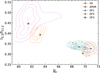 |
Fig. 11 Correlation between the I3.3/I11.2 PAH size proxy and |


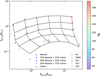 |
Fig. 12 PAH charge-size grid (Maragkoudakis et al. 2020) providing an alternative, fitting-independent description to the charge state and |

4 Discussion
The NASA Ames pyPAHdb is a convenient and efficient spectral modelling tool focused on the analysis of JWST spectral mosaics. It provides the means to model the PAH emission spectrum of astronomical sources using emission spectra of individual PAHs. pyPAHdb delivers maps of the different PAH charge states and size components from the PAH molecules contributing to the fit, along with maps of the PAH ionisation parameter γ and  . Utilising pyPAHdb, we have modelled 5− 15 μm PAH emission spectra across the Orion Bar, obtained from the decomposition of the PDRs4All MIRI-MRS mosaic observations, revealing the fractional contribution of different PAH charge states and different-sized PAHs to the total PAH emission.
With a larger influx of UV photons at the edge of the PDR, PAH cations are expected to be at a higher concentration in the APDR zone following the IF, gradually decreasing towards the molecular cloud zone as UV photons become attenuated, and consequently the concentration of neutral PAHs increases. pyPAHdb modelling supports this picture, where the peak of the fractional contribution of PAH cations is found in the APDR zone and neutral PAHs make a minimum contribution. Accordingly, high fneut values are observed in the face-on emission of the H II region and background molecular cloud regions past DF2, where UV photons are sufficiently attenuated to decrease the rate of PAH ionisation. Further corroboration is found from the peak of PAH anion emission, which is observed deep within the DF2 and DF3 zones. The higher fractions of PAH cations (and lower fractions of PAH anions) in BDF3 than towards DF3 further support the hypothesis that a significant component of PAH emission towards BDF3 may arise from layers not directly associated with the Bar itself.
In regions of high radiation field intensities, photodissociation and photodestruction of small PAHs is expected to actively take place (e.g. Joblin et al. 1996; Berné et al. 2015; Peeters et al. 2024; Chown et al. 2024). pyPAHdb modelling results affirm this, with the peak of the fractional contribution of NC ≤ 50 PAHs found between the DF2 and DF3 zones, and their lowest contribution in the IF and H ii region. Overall, small and medium-sized PAHs make up ∼ 70% of the PAH emission across the mosaic, while ∼ 30% is due to large PAHs. In general, the PAH size distribution will be shaped by the interplay between processes such as destruction, fragmentation, and bottom-up formation of PAH molecules. The magnitude of each process will vary depending on the chemical and physical conditions in the local environment, i.e. PAH destruction will be more prevalent in the H II region and the IF, followed by photodissociation and/or fragmentation (or top-down formation, e.g. Cesarsky et al. 2000; Berné et al. 2007; Pilleri et al. 2012) whereby larger PAHs, or small carbonaceous grains, are fragmented to produce medium-sized PAHs, which in turn produce smaller PAHs. This succession can be observed at the border of the IF in the PAH size breakdown maps (Figure 4), where: flar peaks before the IF, fmed is high at the PDR right after the IF, and fsm gradually increases within the APDR zone compared to the H ii zone and IF. The transient presence of trace amounts of C2H in the APDR (Goicoechea et al. 2025) provides further support for photodestruction of PAHs in this region, as laboratory experiments show that photodestruction of PAHs produces C2H2 (Jochims et al. 1994; Ekern et al. 1998; Zhen et al. 2015) and photodissociation of C2H2 produces C2H (Cheng et al. 2011; Heays et al. 2017). Within the APDR and up to the DF2 the size distribution is balanced with an even contribution (30−35%) from different-sized molecules. Beyond DF2, where photodissociation or fragmentation are less likely to occur due to the drop in the UV intensity, a bottom-up PAH formation may take place, whereby intermediate and large PAHs are formed, at different rates, from the pool of NC ≤ 50 PAHs and by the enhanced abundances of small hydrocarbon radicals (e.g. Goicoechea et al. 2025). This can be seen in the PAH size breakdown maps (Figure 4) between DF2 and DF3, and especially at DF3.
The derived γ across the mosaic ranges between ∼ 2−9 × 10⁴ K1/2 cm−3, which fall between the values reported by Berné et al. (2022a) of (0.7−2.0 × 10⁴) K1/2 cm−3 based on model results from Joblin et al. (2018), and 10.4 × 10⁴ K1/2 cm−3 derived from the NIRSpec observations (Peeters et al. 2024). At the IF γ is on average 4.4 × 10⁴ K1/2 cm−3, which is in agreement with Salgado et al. (2016) (γ=4 × 10⁴ K1/2 cm−3), who assumed a constant temperature (Tgas=500 K) and electron density (ne=15 cm−3), with G0 estimated from the incident radiation field attenuated in the Bar. Similarly at the position of the H2 peak, roughly at DF3, Salgado et al. (2016) reported γ=1.5 × 10⁴ K1/2 cm−3 and pyPAHdb analysis derived γ=3.5 × 10⁴ K1/2 cm−3. The derived γ in this work is dependent on the adopted multiplication factor for the density ratio of cation to neutral PAHs (Eq. (1)), which in this case is taken for circumcoronene (NC=54). Although the average PAH size across the mosaic is somewhat similar,  = 67, applying a single factor for a distribution of PAH sizes may be less appropriate, explaining perhaps some of the variation in γ with the previous works.
Currently, pyPAHdb can very successfully model the 5–15 μm JWST PAH spectrum. The inclusion of the 3.3−3.4 μm bands for simultaneous modelling of the 3−15 μm PAH spectrum would allow the carriers at the low end of the PAH size distribution to be sampled in more detail. Modelling of these shorter wavelength bands at 3.3−3.4 μm requires implementation of anharmonic vibrational spectroscopy of PAHs (Esposito et al. 2024a)8. The term ‘anharmonicity’ as used here refers to the inclusion of higher-order terms (e.g. cubic and quartic) in the vibrational calculation that lead to more accurate vibrational frequencies as well as the treatment of resonances and mode coupling that redistributes band intensities and introduces new bands (e.g. at 5.25 and 5.7 μm Boersma et al. 2009). Indeed, it has been shown that the positions and profiles of the astronomical 3.3 and 3.4 μm bands can only be reproduced with treatment of anharmonicity in the computations (Mackie et al. 2016; Maltseva et al. 2018). Furthermore, the weak but many overtone and combination bands produce a so-called PAH-continuum that spans 3−5 μm and anharmonic results also suggest that the separation of the 3.3−3.4 μm aromatic and aliphatic PAH features is less straightforward than initially thought (Allamandola et al. 2021; Boersma et al. 2023; Esposito et al. 2024b). Together, this severely complicates analysing the astronomical 3−6 μm PAH spectrum. Nonetheless, at first order, sampling of the lower end of the PAH size distribution via the 3.3 μm PAH feature would provide additional constraints in the pyPAHdb-derived PAH size determinations.
The I6.2/I11.2, I7.7/I11.2, and I8.6/I11.2 PAH intensity ratios, which are empirical tracers of PAH ionisation, scale extremely well with γ (Figure 10). This correlation is effectively linear for PAH emission in the H ii zone (which emanates from the background face-on PDR), the APDR zone, across DF1 and up to DF2. Two separate linear branches are seen in the γ−I6.2,7.7/I11.2 relations, which include: i) regions in the H ii zone and the APDR template (bottom branch); ii) regions in the APDR zone (excluding the APDR template) and up to the DF2, as well as regions beyond DF3 (top branch). In the γ−I8.6/I11.2 case, the two branches are absent (or merged). Such variation in the γ−IX/I11.2 relations, i.e. the presence (or absence) of branches, is the result of variation in the PAH intensity ratios in the different zones, which could reflect variations in the carriers of the 6.2, 7.7, and 8.6 μm emission, but also variations due to extinction (Peeters et al. 2024). In the molecular cloud zone, between DF2 and DF3, γ and IX/I11.2 do not correlate. This marks a distinction between PAH ionisation as traced empirically and via spectral modelling, in regions of dominant PDR emission (H ii, APDR, and potentially part of the BDF3 zones) and regions within the molecular cloud. Within the DF2-DF3 zones, the PAH intensity ratios have the largest variation (Figure 9) when compared to the other zones, whereas γ estimated from pyPAHdb modelling has a confined range at lower values (between 3−4.5 × 10⁴) in comparison to zones closer to the IF. This is a clear case in which empirical tracers involving PAH intensity ratios of two bands cannot efficiently describe PAH ionisation, whereas modelling of the entire 5−15 μm PAH spectrum provides a detailed characterisation of the net contribution of neutral and cationic PAHs within the different PAH bands.
5 Conclusions
Using the NASA Ames pyPAHdb spectral modelling tool, we have modelled 5−15 μm PAH emission spectra across the PDRs4All Orion Bar MIRI-MRS mosaic, including the five key physical zones, i.e. the H ii region, the APDR, and the three bright H i/H2 DFs (DF1, DF2, and DF3) corresponding to three molecular hydrogen (H2) filaments. The main conclusions from our work are summarised below:
- (i)
Cationic PAH emission peaks in the APDR region (60–70%), where neutral PAHs make a minimal contribution (up to ∼ 25%). Emission from neutral PAHs peaks in the line of sight towards the H ii region (40−50%), originating in a background face-on PDR, and from the underlying molecular cloud regions past DF2 (∼ 40%). The PAH anions are observed (up to ∼ 20%) deep within the DF2 and DF3 zones. The PAH ionisation parameter, γ, ranges between ∼ 2−9 × 10⁴ across the mosaic;
- (ii)
Small (NC ≤ 50) and medium (50<NC ≤ 70)-sized PAHs make up ∼ 70% of the PAH emission across the mosaic, with the peak of the small PAH emission (45%−50%) found between DF2 and DF3. The average PAH size NC across the Orion Bar ranges between ~60-74;
- (iii)
The fractional PAH charge and size breakdown from pyPAHdb modelling reveals regions of likely top-down PAH formation at the IF, and bottom-up PAH formation within the molecular cloud region;
- (iv)
The derived average PAH size NC in the different physical zones is consistent with a scenario in which PAHs are being more extensively subjected to ultraviolet processing closer to the IF, and less within the molecular cloud;
- (v)
Empirical tracers for PAH ionisation scale well with γ in regions dominated by PDR emission, but their correlation weakens within the molecular cloud zone. Therefore, modelling of the 5−15 μm PAH spectrum with pyPAHdb achieves comprehensive characterisation of the net contribution of neutral and cationic PAHs across different environments, whereas empirical PAH intensity ratio tracers can be highly variable and less reliable outside regions dominated by PDR emission.
Data availability
The dataset maps are available at the CDS via https://cdsarc.cds.unistra.fr/viz-bin/cat/J/A+A/709/A38
Acknowledgements
We would like to thank the referee for providing constructive comments and suggestions that have improved the clarity of this paper. A.M., L.J.A., V.J.E., and J.D.B.’s research was supported by an appointment at NASA Ames Research Center, administered by the Bay Area Environmental Research Institute (80NSSC23M0028). C.B. is grateful for an appointment at NASA Ames Research Center through the San José State University Research Foundation (80NSSC22M0107). A.M., C.B., L.J.A., P.T., V.J.E., J.D.B., and A.R. gratefully acknowledge support from the “NASA Ames Laboratory Astrophysics Directed Work Package (LADWP) Round 2 ISFM” (22-A22ISFM0009). E.P. acknowledges support from the University of Western Ontario, the Canadian Space Agency (CSA, 22JWGO1-16), and the Natural Sciences and Engineering Research Council of Canada. J.R.G. thanks the Spanish MCINN for funding support under grant PID2023-146667NB-I00. A.F. acknowledges funding from the European Research Council (ERC) under the European Union’s Horizon Europe research and innovation programme ERC-AdG-2022 (GA No. 101096293) A.F. also thanks project PID2022-137980NB-I00 funded by the Spanish Ministry of Science and Innovation/State Agency of Research MCIN/AEI/10.13039/501100011033 and by “ERDF A way of making Europe”. M.B. acknowledges DST, India for the ‘DST INSPIRE Faculty’ fellowship and grant. M.B. also acknowledges IUCAA, Pune for visiting associateship.
References
- Allamandola, L. J., Boersma, C., Lee, T. J., Bregman, J. D., & Temi, P., 2021, ApJ, 917, L35 [CrossRef] [Google Scholar]
- Allamandola, L. J., Tielens, A. G. G. M., & Barker, J. R., 1985, ApJ, 290, L25 [Google Scholar]
- Allamandola, L. J., Tielens, A. G. G. M., & Barker, J. R., 1989, ApJS, 71, 733 [Google Scholar]
- Allamandola, L. J., Hudgins, D. M., & Sandford, S. A., 1999, ApJ, 511, L115 [Google Scholar]
- Andrews, H., Boersma, C., Werner, M. W., et al. 2015, ApJ, 807, 99 [NASA ADS] [CrossRef] [Google Scholar]
- Bakes, E. L. O., & Tielens, A. G. G. M., 1994, ApJ, 427, 822 [NASA ADS] [CrossRef] [Google Scholar]
- Bally, J., O’Dell, C. R., & McCaughrean, M. J., 2000, AJ, 119, 2919 [NASA ADS] [CrossRef] [Google Scholar]
- Bauschlicher, Jr., C. W., Boersma, C., Ricca, A., et al. 2010, ApJS, 189, 341 [NASA ADS] [CrossRef] [Google Scholar]
- Bauschlicher, Charles W., J., Ricca, A., Boersma, C., & Allamandola, L. J. 2018, ApJS, 234, 32 [NASA ADS] [CrossRef] [Google Scholar]
- Beintema, D. A., van den Ancker, M. E., Molster, F. J., et al. 1996, A&A, 315, L369 [Google Scholar]
- Bernard-Salas, J., Habart, E., Arab, H., et al. 2012, A&A, 538, A37 [NASA ADS] [CrossRef] [EDP Sciences] [Google Scholar]
- Berné, O., Joblin, C., Deville, Y., et al. 2007, A&A, 469, 575 [NASA ADS] [CrossRef] [EDP Sciences] [Google Scholar]
- Berné, O., Foschino, S., Jalabert, F., & Joblin, C. 2022a, A&A, 667, A159 [NASA ADS] [CrossRef] [EDP Sciences] [Google Scholar]
- Berné, O., Habart, É., Peeters, E., et al. 2022b, PASP, 134, 054301 [CrossRef] [Google Scholar]
- Berné, O., Habart, E., Peeters, E., et al. 2024, Science, 383, 988 [Google Scholar]
- Berné, O., Martin-Drumel, M.-A., Schroetter, I., et al. 2023, Nature, 621, 56 [CrossRef] [Google Scholar]
- Berné, O., Montillaud, J., & Joblin, C., 2015, A&A, 577, A133 [NASA ADS] [CrossRef] [EDP Sciences] [Google Scholar]
- Boersma, C., Mattioda, A. L., Bauschlicher, C. W., et al. 2009, ApJ, 690, 1208 [NASA ADS] [CrossRef] [Google Scholar]
- Boersma, C., Bregman, J. D., & Allamandola, L. J., 2013, ApJ, 769, 117 [NASA ADS] [CrossRef] [Google Scholar]
- Boersma, C., Bauschlicher, Jr., C. W., Ricca, A., et al. 2014, ApJS, 211, 8 [NASA ADS] [CrossRef] [Google Scholar]
- Boersma, C., Bregman, J., & Allamandola, L. J., 2015, ApJ, 806, 121 [NASA ADS] [CrossRef] [Google Scholar]
- Boersma, C., Bregman, J., & Allamandola, L. J., 2018, ApJ, 858, 67 [NASA ADS] [CrossRef] [Google Scholar]
- Boersma, C., Allamandola, L. J., Esposito, V. J., et al. 2023, ApJ, 959, 74 [NASA ADS] [CrossRef] [Google Scholar]
- Bregman, J. D., Allamandola, L. J., Tielens, A. G. G. M., Geballe, T. R., & Witteborn, F. C., 1989, ApJ, 344, 791 [NASA ADS] [CrossRef] [Google Scholar]
- Cami, J., 2011, in EAS Publications Series, 46, EAS Publications Series, 117 [Google Scholar]
- Cesarsky, D., Jones, A. P., Lequeux, J., & Verstraete, L., 2000, A&A, 358, 708 [NASA ADS] [Google Scholar]
- Chastenet, J., Sutter, J., Sandstrom, K., et al. 2023, ApJ, 944, L12 [NASA ADS] [CrossRef] [Google Scholar]
- Cheng, B.-M., Chen, H.-F., Lu, H.-C., et al. 2011, ApJS, 196, 3 [NASA ADS] [CrossRef] [Google Scholar]
- Chown, R., Sidhu, A., Peeters, E., et al. 2024, A&A, 685, A75 [NASA ADS] [CrossRef] [EDP Sciences] [Google Scholar]
- Croiset, B. A., Candian, A., Berné, O., & Tielens, A. G. G. M., 2016, A&A, 590, A26 [NASA ADS] [CrossRef] [EDP Sciences] [Google Scholar]
- Draine, B. T., & Li, A., 2007, ApJ, 657, 810 [CrossRef] [Google Scholar]
- Draine, B. T., Li, A., Hensley, B. S., et al. 2021, ApJ, 917, 3 [CrossRef] [Google Scholar]
- Egorov, O. V., Kreckel, K., Sandstrom, K. M., et al. 2023, ApJ, 944, L16 [NASA ADS] [CrossRef] [Google Scholar]
- Ekern, S. P., Marshall, A. G., Szczepanski, J., & Vala, M., 1998, J. Phys. Chem. A, 102, 3498 [NASA ADS] [CrossRef] [Google Scholar]
- Esposito, V. J., Allamandola, L. J., Boersma, C., et al. 2024a, Mol. Phys., 122, e2252936 [Google Scholar]
- Esposito, V. J., Bejaoui, S., Billinghurst, B. E., et al. 2024b, MNRAS, 535, 3239 [Google Scholar]
- Galliano, F., Madden, S. C., Tielens, A. G. G. M., Peeters, E., & Jones, A. P., 2008, ApJ, 679, 310 [Google Scholar]
- García-Bernete, I., Rigopoulou, D., Alonso-Herrero, A., et al. 2022, A&A, 666, L5 [NASA ADS] [CrossRef] [EDP Sciences] [Google Scholar]
- Goicoechea, J. R., Pety, J., Cuadrado, S., et al. 2016, Nature, 537, 207 [Google Scholar]
- Goicoechea, J. R., Santa-Maria, M. G., Bron, E., et al. 2019, A&A, 622, A91 [NASA ADS] [CrossRef] [EDP Sciences] [Google Scholar]
- Goicoechea, J. R., Pety, J., Cuadrado, S., et al. 2025, A&A, 696, A100 [NASA ADS] [CrossRef] [EDP Sciences] [Google Scholar]
- Habart, E., Peeters, E., Berné, O., et al. 2024, A&A, 685, A73 [NASA ADS] [CrossRef] [EDP Sciences] [Google Scholar]
- Habing, H. J., 1968, Bull. Astron. Inst. Netherlands, 19, 421 [Google Scholar]
- Haworth, T. J., Reiter, M., O’Dell, C. R., et al. 2023, MNRAS, 525, 4129 [NASA ADS] [CrossRef] [Google Scholar]
- Heays, A. N., Bosman, A. D., & van Dishoeck, E. F., 2017, A&A, 602, A105 [NASA ADS] [CrossRef] [EDP Sciences] [Google Scholar]
- Hogerheijde, M. R., Jansen, D. J., & van Dishoeck, E. F., 1995, A&A, 294, 792 [NASA ADS] [Google Scholar]
- Hony, S., Van Kerckhoven, C., Peeters, E., et al. 2001, A&A, 370, 1030 [CrossRef] [EDP Sciences] [Google Scholar]
- Joblin, C., Tielens, A. G. G. M., Allamandola, L. J., & Geballe, T. R., 1996, ApJ, 458, 610 [NASA ADS] [CrossRef] [Google Scholar]
- Joblin, C., Bron, E., Pinto, C., et al. 2018, A&A, 615, A129 [NASA ADS] [CrossRef] [EDP Sciences] [Google Scholar]
- Jochims, H. W., Ruhl, E., Baumgartel, H., Tobita, S., & Leach, S., 1994, ApJ, 420, 307 [NASA ADS] [CrossRef] [Google Scholar]
- Kassis, M., Adams, J. D., Campbell, M. F., et al. 2006, ApJ, 637, 823 [NASA ADS] [CrossRef] [Google Scholar]
- Khan, B., Abbott, B., Peeters, E., et al. 2025a, A&A, 699, A133 [NASA ADS] [CrossRef] [EDP Sciences] [Google Scholar]
- Khan, B., Daza Rodriguez, S. A., Peeters, E., et al. 2025b, arXiv e-prints [arXiv:2510.06167] [Google Scholar]
- Knight, C., Peeters, E., Stock, D. J., Vacca, W. D., & Tielens, A. G. G. M., 2021, ApJ, 918, 8 [NASA ADS] [CrossRef] [Google Scholar]
- Knight, C., Peeters, E., Tielens, A. G. G. M., & Vacca, W. D., 2022, MNRAS, 509, 3523 [Google Scholar]
- Lai, T. S. Y., Armus, L., U, V., et al. 2022, ApJ, 941, L36 [NASA ADS] [CrossRef] [Google Scholar]
- Lai, T. S. Y., Armus, L., Bianchin, M., et al. 2023, ApJ, 957, L26 [NASA ADS] [CrossRef] [Google Scholar]
- Leger, A., & Puget, J. L., 1984, A&A, 137, L5 [Google Scholar]
- Mackie, C. J., Candian, A., Huang, X., et al. 2016, J. Chem. Phys., 145, 084313 [NASA ADS] [CrossRef] [Google Scholar]
- Maltseva, E., Mackie, C. J., Candian, A., et al. 2018, A&A, 610, A65 [NASA ADS] [CrossRef] [EDP Sciences] [Google Scholar]
- Maragkoudakis, A., Ivkovich, N., Peeters, E., et al. 2018, MNRAS, 481, 5370 [CrossRef] [Google Scholar]
- Maragkoudakis, A., Peeters, E., & Ricca, A., 2023a, MNRAS, 520, 5354 [NASA ADS] [CrossRef] [Google Scholar]
- Maragkoudakis, A., Peeters, E., Ricca, A., & Boersma, C., 2023b, MNRAS, 524, 3429 [Google Scholar]
- Maragkoudakis, A., Peeters, E., & Ricca, A., 2020, MNRAS, 494, 642 [NASA ADS] [CrossRef] [Google Scholar]
- Maragkoudakis, A., Boersma, C., Temi, P., Bregman, J. D., & Allamandola, L. J., 2022, ApJ, 931, 38 [CrossRef] [Google Scholar]
- Maragkoudakis, A., Boersma, C., Temi, P., et al. 2025, ApJ, 979, 90 [Google Scholar]
- Mattioda, A. L., Hudgins, D. M., Boersma, C., et al. 2020, ApJS, 251, 22 [NASA ADS] [CrossRef] [Google Scholar]
- Parikka, A., Habart, E., Bernard-Salas, J., Köhler, M., & Abergel, A., 2018, A&A, 617, A77 [NASA ADS] [CrossRef] [EDP Sciences] [Google Scholar]
- Pasquini, S., Peeters, E., Schefter, B., et al. 2024, A&A, 685, A77 [NASA ADS] [CrossRef] [EDP Sciences] [Google Scholar]
- Peeters, E., Hony, S., Van Kerckhoven, C., et al. 2002a, A&A, 390, 1089 [NASA ADS] [CrossRef] [EDP Sciences] [Google Scholar]
- Peeters, E., Martín-Hernández, N. L., Damour, F., et al. 2002b, A&A, 381, 571 [NASA ADS] [CrossRef] [EDP Sciences] [Google Scholar]
- Peeters, E., Spoon, H. W. W., & Tielens, A. G. G. M., 2004, ApJ, 613, 986 [NASA ADS] [CrossRef] [Google Scholar]
- Peeters, E., Bauschlicher, Jr., C. W., Allamandola, L. J., et al. 2017, ApJ, 836, 198 [NASA ADS] [CrossRef] [Google Scholar]
- Peeters, E., Habart, E., Berné, O., et al. 2024, A&A, 685, A74 [NASA ADS] [CrossRef] [EDP Sciences] [Google Scholar]
- Pilleri, P., Montillaud, J., Berné, O., & Joblin, C., 2012, A&A, 542, A69 [NASA ADS] [CrossRef] [EDP Sciences] [Google Scholar]
- Pilleri, P., Joblin, C., Boulanger, F., & Onaka, T., 2015, A&A, 577, A16 [NASA ADS] [CrossRef] [EDP Sciences] [Google Scholar]
- Ricca, A., Bauschlicher, Charles W., J., Boersma, C., Tielens, A. G. G. M., & Allamandola, L. J. 2012, ApJ, 754, 75 [NASA ADS] [CrossRef] [Google Scholar]
- Rigopoulou, D., Donnan, F. R., García-Bernete, I., et al. 2024, arXiv e-prints [arXiv:2406.11415] [Google Scholar]
- Salgado, F., Berné, O., Adams, J. D., et al. 2016, ApJ, 830, 118 [Google Scholar]
- Sandstrom, K. M., Bolatto, A. D., Bot, C., et al. 2012, ApJ, 744, 20 [CrossRef] [Google Scholar]
- Schutte, W. A., Tielens, A. G. G. M., & Allamandola, L. J., 1993, ApJ, 415, 397 [NASA ADS] [CrossRef] [Google Scholar]
- Shannon, M. J., & Boersma, C., 2018, in Proceedings of the 17th Python in Science Conference (SciPy), 99 [Google Scholar]
- Smith, J. D. T., Draine, B. T., Dale, D. A., et al. 2007, ApJ, 656, 770 [Google Scholar]
- Stock, D. J., & Peeters, E., 2017, ApJ, 837, 129 [NASA ADS] [CrossRef] [Google Scholar]
- Stock, D. J., Choi, W. D.-Y., Moya, L. G. V., et al. 2016, ApJ, 819, 65 [NASA ADS] [CrossRef] [Google Scholar]
- Tielens, A. G. G. M., 2005, The Physics and Chemistry of the Interstellar Medium (Cambridge: Cambridge University Press) [Google Scholar]
- Tielens, A. G. G. M., Meixner, M. M., van der Werf, P. P., et al. 1993, Science, 262, 86 [NASA ADS] [CrossRef] [Google Scholar]
- Van De Putte, D., Meshaka, R., Trahin, B., et al. 2024, A&A, 687, A86 [NASA ADS] [CrossRef] [EDP Sciences] [Google Scholar]
- Van De Putte, D., Peeters, E., Gordon, K. D., et al. 2025, A&A, 701, A111 [NASA ADS] [CrossRef] [EDP Sciences] [Google Scholar]
- Vicente, S., Berné, O., Tielens, A. G. G. M., et al. 2013, ApJ, 765, L38 [NASA ADS] [CrossRef] [Google Scholar]
- Werner, M. W., Uchida, K. I., Sellgren, K., et al. 2004, ApJS, 154, 309 [Google Scholar]
- Zang, R. X., Maragkoudakis, A., & Peeters, E., 2022, MNRAS, 511, 5142 [Google Scholar]
- Zhen, J., Castellanos, P., Paardekooper, D. M., et al. 2015, ApJ, 804, L7 [Google Scholar]
The effects of different modelling configurations and PAHdb library versions on the results have been extensively examined in Maragkoudakis et al. (2025).
Anharmonic spectra of PAHs are to be added to PAHdb in a forthcoming release.
Appendix A pyPAHdb modelling error
The pyPAHdb modelling error (σpyPAHdb) is quantified as the ratio between the integrals of the absolute residuals over that of the absolute input spectrum (e.g. Bauschlicher et al. 2018; Maragkoudakis et al. 2022, 2025). The map of σpyPAHdb is presented in Figure A.1. Regions of relatively high σpyPAHdb (>0.30) are seen in the 203-504 proplyd and part of the H ii region, whereas the mean σpyPAHdb is 0.13 ± 0.03, similarly to the average modelling error ( =0.16) obtained for nearby galaxies (Maragkoudakis et al. 2025).
 |
Fig. A.1 The pyPAHdb modelling error (σpyPAHdb) map. |
Appendix B pyPAHdb modelling of the five key physical zones
Modelling to the weighted averaged (template) spectrum of each of the five key physical zones was performed with pyPAHdb (Section 3.4). The plots of the PAH charge and size breakdown for the APDR and DF3 regions are presented in Figure 2 and for the HII, DF1, and DF3 regions in Figure B.1.
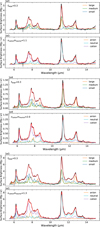 |
Fig. B.1 The pyPAHdb PAH size and charge breakdown of the spectral templates of the H ii (top), DF1 (middle), and DF2 (bottom) regions. Observations are shown in black, total fit in red, and the separate breakdown components are given in the legend of each panel. The fractions of the large PAH contributing to the fit and the cation-to-neutral PAHs ratio are provided as labels. |
All Tables
pyPAHdb derived parameters for the five template spectra (H ii APDR, DF 1, DF 2, and DF 3) and average parameter values of the regions between the key physical zones (H ii-IF, APDR-DF1, DF1-DF2, DF2-DF3, and DF3-BDF3).
All Figures
|
Fig. 1 Spectral decomposition of the five Orion Bar template spectra in the 5−15 μm wavelength region. The template spectra are shown in blue, the spectrum after the emission lines removal is shown in orange, the fitted baseline in green, and the resulting isolated PAH emission spectrum in red. |
| In the text | |
|
Fig. 2 PAH size (top sub-panels) and charge breakdown (bottom sub-panels) for the spectral templates of the APDR (left) and DF3 (right). Observations are shown in black and the total fit in red, and the separate breakdown components are given in the legend of each panel. |
| In the text | |
|
Fig. 3 PAH charge breakdown maps. The map of neutral PAHs is shown in the top panel, the PAH cations map in the middle panel, and the PAH anions map in the bottom panel. The colour bar shows the respective charge fractions, and for each map the range is scaled between the 0.5% and 99.5% percentiles. The colour map has been chosen to emphasise structure. |
| In the text | |
|
Fig. 4 PAH size breakdown maps. The map of large PAHs (NC<70) is shown in the top panel, the medium-sized PAHs (50<NC ≤ 70) map in the middle panel, and the small PAHs (NC ≤ 50) in the bottom panel. The colour bar shows the respective size fractions, and for each map the range is scaled between the 0.5% and 99.5% percentiles. |
| In the text | |
|
Fig. 5 Map of the PAH ionisation parameter (γ) obtained from the pyPAHdb modelling. White lines indicate the IF and the three DFs. |
| In the text | |
|
Fig. 6 Map of the average NC obtained from pyPAHdb modelling. White lines indicate the IF and the three DFs. |
| In the text | |
|
Fig. 7 Wavelength regions adopted for the measurement of the different PAH emission intensities, as deduced from the five spectral templates. The wavelength intervals are defined as follows: PAH6.2 μm: 6.0−6.6 μm; PAH7.7 μm: 7.0−8.2 μm; PAH8.6 μm: 8.2−9.15 μm; and PAH11.2 μm: 11.1− 11.7 μm. |
| In the text | |
|
Fig. 8 Maps of the 6.2 μm 7.7 μm, 8.6 μm, and 11.2 μm PAH flux (in erg s−1 cm−2). The rectangular apertures of the five template regions are indicated, along with lines for the IF and DFs. |
| In the text | |
|
Fig. 9 PAH band intensity ratio maps. The rectangular apertures of the five template regions are indicated, along lines for the IF and DFs. |
| In the text | |
|
Fig. 10 Correlations between the different empirical PAH ionisation proxies (I6.2/I11.2, left panels; I7.7/I11.2, middle panels; I8.6/I11.2, right panels) and the PAH ionisation parameter (γ) deduced from pyPAHdb modelling. In the top panels, the pixels are colour-coded based on their vertical distance from the edge of the mosaic, which is indicative of the projected distance from θ1 Ori C. In the bottom panels, pixels corresponding to each of the five key physical regions are assigned a specific colour (H ii in green, APDR in red, DF1 in blue, DF2 in orange, and DF3 in pink), with the average values from each template indicated with a different symbol. Pixels outside the five zones are shown in grey. |
| In the text | |
|
Fig. 11 Correlation between the I3.3/I11.2 PAH size proxy and |
| In the text | |
|
Fig. 12 PAH charge-size grid (Maragkoudakis et al. 2020) providing an alternative, fitting-independent description to the charge state and |
| In the text | |
|
Fig. A.1 The pyPAHdb modelling error (σpyPAHdb) map. |
| In the text | |
|
Fig. B.1 The pyPAHdb PAH size and charge breakdown of the spectral templates of the H ii (top), DF1 (middle), and DF2 (bottom) regions. Observations are shown in black, total fit in red, and the separate breakdown components are given in the legend of each panel. The fractions of the large PAH contributing to the fit and the cation-to-neutral PAHs ratio are provided as labels. |
| In the text | |
Current usage metrics show cumulative count of Article Views (full-text article views including HTML views, PDF and ePub downloads, according to the available data) and Abstracts Views on Vision4Press platform.
Data correspond to usage on the plateform after 2015. The current usage metrics is available 48-96 hours after online publication and is updated daily on week days.
Initial download of the metrics may take a while.