| Issue |
A&A
Volume 708, April 2026
|
|
|---|---|---|
| Article Number | A313 | |
| Number of page(s) | 22 | |
| Section | Planets, planetary systems, and small bodies | |
| DOI | https://doi.org/10.1051/0004-6361/202556822 | |
| Published online | 21 April 2026 | |
Long-term monitoring of WASP-19 b: Signs of apsidal precession and molecular signatures
1
Instituto de Astronomía y Ciencias Planetarias de Atacama (INCT), Universidad de Atacama,
Copayapu 485,
Copiapó,
Chile
2
European Southern Observatory,
Karl-Schwarzschild-Straße 2,
85748
Garching bei München,
Germany
3
Department of Physics, Washington University,
St. Louis,
MO
63130,
USA
4
School of Earth and Space Sciences, University of Science and Technology of China,
Hefei
230026,
China
5
Centro de Astronomía (CITEVA), Universidad de Antofagasta, Avenida U. de Antofagasta,
02800
Antofagasta,
Chile
6
Astrophyscis Group, Keele University,
Staffordshire
ST5 5BG,
UK
7
University of Southern Denmark, Department of Physics, Chemistry and Pharmacy,
SDU-Galaxy, Campusvej 55,
5230
Odense M,
Denmark
8
Centre for Astrophysics Research, Department of Physics, Astronomy and Mathematics, University of Hertfordshire,
College Lane,
Hatfield
AL10 9AB,
UK
9
Institute for Astronomy, University of Edinburgh,
Royal Observatory,
Edinburgh
EH9 3HJ,
UK
10
Centre for ExoLife Sciences, Niels Bohr Institute,
Jagtvej 155,
2200
Copenhagen,
Denmark
11
INAF - Osservatorio Astrofisico di Torino,
Via Observatorio 20,
10025
Pino Torinese,
Italy
12
Alma Mater Studiorum - University of Bologna, Dipartimento di Fisica e Astronomia “Augusto Righi”,
Via Gobetti 93/2,
40129
Bologna,
Italy
13
Istituto Nazionale di Fisica Nucleare, Sezione di Napoli,
Napoli,
Italy
14
Earth System Sciences, Atmospheric Science, University of Hamburg,
Hamburg,
Germany
15
Centre for Exoplanet Science, SUPA, School of Physics & Astronomy, University of St Andrews,
North Haugh,
St Andrews
KY16 9SS,
UK
16
Millennium Institute of Astrophysics MAS,
Nuncio Monsenor Sotero Sanz 100, Of. 104,
Providencia,
Santiago,
Chile
17
Instituto de Astrofísica, Facultad de Física, Pontificia Universidad Católica de Chile,
Av. Vicuña Mackenna 4860,
7820436
Macul,
Santiago,
Chile
18
Astronomisches Rechen-Institut, Zentrum für Astronomie der Universität Heidelberg (ZAH),
69120
Heidelberg,
Germany
19
Astronomy Research Center, Research Institute of Basic Sciences, Seoul National University,
1 Gwanak-ro,
Gwanak-gu,
Seoul
08826,
Korea
20
Max-Planck-Institut für Astronomie,
Königstuhl 17,
69117
Heidelberg,
Germany
21
European Southern Observatory (ESO),
Alonso de Córdova 3107
Vitacura,
Santiago,
Chile
22
Departamento de Matemática y Física Aplicadas, Facultad de Ingeniería, Universidad Católica de la Santísima Concepción,
Alonso de Rivera
2850,
Concepción,
Chile
23
Perimeter Institute for Theoretical Physics,
31 Caroline St N,
Waterloo,
ON
N2L 2Y5,
Canada
24
Centre for Electronic Imaging, Department of Physical Sciences, The Open University,
Milton Keynes
MK7 6AA,
UK
25
Dipartimento di Fisica, Università degli Studi di Roma Tor Vergata,
via della Ricerca Scientifica 1,
00133,
Roma,
Italy
★ Corresponding author: This email address is being protected from spambots. You need JavaScript enabled to view it.
Received:
11
August
2025
Accepted:
9
February
2026
Abstract
Context. With over 6000 exoplanets discovered to date, approximately 12 % are classified as hot-Jupiters. Due to their large sizes and short orbital periods (P < 10 day), they are easier to detect and provide crucial insights into planetary formation, atmospheric properties, and orbital dynamics. Among these, ultra-short-period exoplanets (P ≤ 1 d) are particularly interesting, as they are expected to undergo orbital decay driven by strong tidal interactions. Despite theoretical predictions, WASP-12 b and WASP-4 b remain the confirmed hot-Jupiters experiencing measurable orbital decay.
Aims. This study presents a homogeneous analysis of WASP-19 b to investigate both its orbital dynamics and atmospheric composition. Leveraging a 15-year dataset, our goal is to assess whether the system exhibits long-term deviations from a constant orbital period and to investigate whether any detected variations are consistent with tidal orbital decay, apsidal precession, or periodic signals indicative of a potential planetary perturber. Additionally, we also construct a photometric transmission spectrum to characterize its atmosphere.
Methods. We analyze multi-wavelength light curves, incorporating starspot modeling with PRISM to account for stellar inhomogeneities. To assess orbital evolution, we fit linear, quadratic, and cubic ephemeris models to transit timing residuals with respect to a non-decaying orbit.
Results. Our analysis, which includes 27 new transits, reveals no statistically significant periodic signal in the transit timings. Although none of the tested ephemeris models fully reproduce the observed timing scatter, the mid-transit times exhibit systematic deviations from a strictly constant orbital period and are best reproduced by the cubic ephemeris in a relative model-comparison sense, indicating a slow, non-periodic long-term trend over the ~ 15-year baseline. This behavior is more consistent with gradual orbital precession than with monotonic tidal decay, for which a dominant quadratic trend would be expected. Fitting a precession model yields a rate of ω̇obs = (1.00 ± 0.12) × 10−4 rad/orbit, corresponding to a planetary Love number k2p = 0.107 ± 0.08, in agreement with recent independent estimates. The transmission spectrum reveals signatures of Na, K, and H2O, with no strong evidence of TiO/VO, likely due to the resolution limits of the photometric data.
Conclusions. Our results support that apsidal precession could be the dominant process governing the long-term orbital evolution of WASP-19b, possibly sustained by weak eccentricity forcing from the wide companion WASP-19 B. These orbital dynamics can, in turn, impact the atmospheric structure by modulating the irradiation history, potentially altering molecular abundances over time. Our findings highlight the importance of combining TTV analyzes with multi-wavelength atmospheric data, while emphasizing that additional high-quality timing and spectroscopic observations are required to corroborate the fidelity of the proposed orbital model.
Key words: techniques: photometric / techniques: spectroscopic / planets and satellites: atmospheres / planets and satellites: dynamical evolution and stability / planet-star interactions
© The Authors 2026
 Open Access article, published by EDP Sciences, under the terms of the Creative Commons Attribution License (https://creativecommons.org/licenses/by/4.0), which permits unrestricted use, distribution, and reproduction in any medium, provided the original work is properly cited.
This article is published in open access under the Subscribe to Open model. This email address is being protected from spambots. You need JavaScript enabled to view it. to support open access publication.
1 Introduction
The discovery of the first hot-Jupiter, 51 Pegasi b, raised numerous unresolved questions regarding established theories of planetary formation and the mechanisms driving the migration and orbital decay of short-period gas giant planets (Mayor & Queloz 1995). Planetary system formation remains an active area of research, with two widely accepted theories proposing that Jupiter-like planets form either via core accretion (Pollack et al. 1996) and/or through gravitational instability (Boss 1997), typically at significant distances from the host star.
In the core accretion (CA) model, dust particles in the protoplan-etary disk coagulate into planetesimals, which grow into solid planetary cores; once these reach a critical mass of ∼10 M⊕, they begin accreting gas from the disk (Mordasini 2018). However, the short lifetime of protoplanetary disks (∼1-10Myr; Haisch et al. 2001) presents a major challenge to this model, particularly for the timely formation of gas giants. This has led to the introduction of the pebble accretion mechanism, which significantly accelerates core growth by allowing centimeter- to metersized particles to be efficiently captured by planetary embryos (Lambrechts & Johansen 2014; Bitsch et al. 2015). Alternatively, the gravitational instability (GI) model suggests that in massive and rapidly cooling disks, direct fragmentation into self-gravitating clumps can occur (Boss 1997); however, GI is often limited by its requirement for very high disk masses and efficient cooling, making it less favored for forming close-in planets. These regions in the disk, rich in condensed material, provide favorable conditions for the onset of such formation processes. Subsequently, the resulting planets migrate inward to close-in orbits (<0.05 au) through a variety of mechanisms, such as planet-planet scattering (Chatterjee et al. 2008), high eccentricity migration (Rasio & Ford 1996), or interactions with the gas disk itself (Paardekooper et al. 2023).
Once these planets reach extremely close-in orbits, they are subjected to intense tidal forces from their host stars, which lead to gradual orbital evolution. The physical mechanism of tidal decay in hot-Jupiter systems involves the transfer of energy and angular momentum between the planet and its host star due to the mutual gravitational interaction (Hebb et al. 2010; Patra et al. 2017; Maciejewski et al. 2018; Mathis 2019). As hot-Jupiters orbit very close to their host star (P < 10 d), the gravitational pull is stronger on the side of the planet facing the star compared to the side facing away from it. This variation in gravitational force leads to a distortion of the planet’s shape. As the planet undergoes this deformation, it tries to adapt to the gravitational pull by reshaping itself. However, this continuous reshaping of the planet results in the generation of internal heat within the planet through tidal dissipation (e.g., Gu et al. 2003; Ogilvie & Lin 2004). The heat generated by tidal dissipation represents a conversion of orbital energy into thermal energy within the planet. This process can contribute to the inflation of the gaseous envelope; however, current inflation models do not fully reproduce the observed radii of all hot-Jupiters, implying that tidal heating is only one of several mechanisms that may operate with varying efficiency across the population. Specifically, when the internal heat increases, it raises the temperature within the planet, reducing the density of the outer layers and causing them to swell. This process of envelope inflation is particularly relevant for hot and ultra-hot Jupiters, where the added thermal energy can significantly alter the planet’s radius and overall structure (Hou & Wei 2022). Moreover, this process affects the planet’s transmission spectrum by modifying vertical temperature gradients and driving atmospheric circulation and influences the abundances of molecular species (Komacek & Showman 2016).
Tidal forces affect the planet’s rotation (Barker et al. 2016), leading to energy loss from its orbital motion and causing its orbit to shrink—a phenomenon known as orbital decay (Ogilvie 2014). This process leads to a shortening of the planet’s orbital period, causing transits to occur earlier than predicted. As the planet’s semi-major axis decreases, it spirals closer to its host star over time. The energy loss also influences the planet’s rotation, driving it toward an aligned spin with its orbit (Gallet et al. 2017), and so becoming tidally locked with its host star. This stellar irradiation drives photochemical processes in the atmosphere of the hot-Jupiters, potentially altering the molecular abundances detectable in the transmission spectrum.
Predicting the long-term orbital evolution of hot-Jupiters remains challenging due to the complex interplay between stellar and planetary properties that influence tidal dissipation. Although intense stellar tides can gradually shrink planetary orbits, potentially leading to planetary engulfment, additional processes, such as magnetic braking (Dawson 2014, and references therein), can further affect orbital alignment and evolution by slowing stellar rotation through the loss of angular momentum to stellar winds. These coupled interactions make it difficult to model decay rates precisely, especially in systems where
unseen companions or evolving stellar interiors may also play a role. However, ultra-short-period systems like WASP-19b (P ≈ 19 hr; Hebb et al. 2010) can enhance our understanding and refine our predictive capabilities, offering valuable insights into the ultimate fate of hot-Jupiters.
Moreover, the study of transmission spectra, when combined with transit timing variations (TTVs), offers a comprehensive approach to understanding the interplay between tidal decay, internal heating, and atmospheric dynamics. By analyzing changes in the transmission spectrum over time, researchers can constrain the chemical and physical processes that occur in the atmosphere as a result of tidal interactions and migration. This is especially important for systems like WASP-19, where the strong tidal forces and close proximity to the host star make these effects particularly significant, and they provide a critical diagnostic for investigating the impact of tidal decay and internal heating on atmospheric composition and structure.
It is, therefore, beneficial to look for TTVs in systems with hot-Jupiters. Population studies have provided some evidence that orbital decay does take place on astrophysically significant timescales - for example WASP-12b Hebb et al. (2010) and WASP-4 b Bastürk et al. (2025) - and the effects of tides are small on human timescales, making it best to focus this search on the most promising systems (Eq. (1), Maciejewski 2019) and (Eq. (5), Birkby et al. 2014). Observations of TTVs can help constrain the efficiency of tidal interactions, track changes in atmospheric features, and improve predictions of the long-term evolution of these systems.
Other mechanisms that can cause a TTV signal include gravitational interactions with additional planets or moons (Ballard et al. 2011), stellar activity (such as starspots or flares; Ioannidis et al. 2016; Sanchis-Ojeda et al. 2011), variations in the planet’s orbital eccentricity and apsidal precession (Antoniciello et al. 2021), Applegate effect (Watson & Marsh 2010), and relativistic effects (Antoniciello et al. 2021).
This paper is structured as follows. In Sect. 2 we describe the hot-Jupiter, WASP-19b. Section 3 describes the observational datasets and the data reduction method. Sect. 4 focuses on the light curve analysis method. Section 5 explores TTV and apsidal motion analysis. In Sect. 6 we present the transmission spectrum and retrieval results. We summarize our results in Sect. 7 and present a discussion and conclusions in Sects. 8 and 9.
2 WASP-19 b
WASP-19b (Hebb et al. 2010) is a Jupiter-like planet (Mp = 1.11 MJup & RP = 1.39 RJup) that orbits an active G8V solar-type star ( M* = 0.9 M⊙, R* = 1.0 R⊙, and an Age ∼11 Gyr) and is one of the first ultra-short-period (P = 0.8 days) planets discovered. The host star shows strong magnetic activity, with a chromospheric index of log R′HK ≈ −4.5 (Doyle et al. 2014) and a coronal X-ray to bolometric luminosity ratio of log(LX/Lbol) ≈ −5.1 (Maggio et al. 2012). In addition, the photometric rotational modulation of ∼0.6-0.8% in the optical flux indicates persistent starspots, with a measured stellar rotation period of ∼10.5 days (Hebb et al. 2010; Mancini et al. 2013).
Since its discovery by Hebb et al. (2010), it has been studied in detail and the planet’s physical properties have been refined and re-determined by several authors (Cortés-Zuleta et al. 2020; Wong et al. 2016; Sing et al. 2016; Tregloan-Reed et al. 2013; Mancini et al. 2013; Hellier et al. 2011; Lendl et al. 2013). In a system like WASP-19, where the stellar rotation period (10.50 ± 0.20 days Hebb et al. 2010) exceeds the orbital period (0.7888396d ± 0.0000010d Hebb et al. 2010), tidal dissipation in the star can transfer angular momentum from the orbit to the stellar spin, causing orbital decay. A few previous studies from Levrard et al. (2009) and Matsumura et al. (2010) predict the significant impact of tidal interactions on the orbital evolution of close-in exoplanets such as WASP-19b. Calculations from Matsumura et al. (2010) have predicted that the orbit of WASP-19b may become unstable due to insufficient total angular momentum, possibly leading to tidal disruption. Valsecchi & Rasio (2014) predicted that, due to the convective damping of equilibrium tides, WASP-19b’s transit arrival times would deviate by at least 34 s from a constant-period ephemeris over a 10-year baseline.
The WASP-19 system is especially interesting to study further, as the host star is known to be highly active with prominent starspots Tregloan-Reed et al. (2013). The presence of a convective envelope in the G8V host star can significantly impact the tidal dissipation processes within the system. Additionally, starspots can introduce systematics that affect the accurate measurement of transit midpoints (Sanchis-Ojeda et al. 2011) and transit depths (Pont et al. 2008). To mitigate these effects, we employ the PRISM (Planetary Retrospective Integrated Starspot Model; Tregloan-Reed et al. 2013, 2015; see our Sect. 4.1) algorithm in our analysis, which allows us to model and account for the impact of starspots on the transit light curves. This allows us to recover the true transit shape and to separate spot-induced anomalies from genuine planetary signals. Through this procedure, we refine the orbital inclination, impact parameter, and mid-transit timing, ensuring that timing residuals are not contaminated by stellar variability. Moreover, by isolating and removing the wavelength-dependent effects of stellar heterogeneity, the derived transmission spectrum becomes more representative of the planetary atmosphere rather than the hoststar surface. Consequently, the inclusion of starspot modeling not only improves the precision of the orbital and transit parameters but also enhances the reliability of atmospheric retrievals. This integrated approach strengthens the link between dynamical evolution and the observed transmission properties of WASP-19 b, providing a self-consistent view of the system’s long-term behavior.
In this work, we present a comprehensive analysis of 27 new, systematically obtained transit observations of WASP-19b from the Danish Telescope and more than 100 transits from TESS, combined with available transit light curves from the literature. This extensive dataset allows us to conduct a long-term, detailed investigation of the evolution of the WASP-19 system over the past two decades. By analyzing these transit observations, we aim to test the predictions of the expected orbital decay of WASP-19b.
3 Observations and data reduction
3.1 Danish 1.54-m telescope
WASP-19b data were collected over a 13 year period, from 2015 to 2023, by the MiNDSTEp collaboration1 using the Danish 1.54-m telescope located at the ESO La Silla Observatory. The observations were performed using the Danish Faint Object Spectrograph and Camera (DFOSC) imager, which has a field of view of 13.7′ × 13.7′ at a plate scale of 0.39" per pixel. However, to decrease the readout time, the charge-coupled device (CCD) was typically windowed to 12′ × 8′. A total of 27 transit light curves were recorded: 14 in the Johnson-Cousins R filter and 13 in the Johnson-Cousins I filter. Two of these (on 26 April 2016 and 20 May 2022) were incomplete and excluded from the final analysis, leaving 25 full transits considered for detailed investigation. The complete set of light curves is presented in Fig. 1. All scientific images were first calibrated using standard CCD reduction procedures. This included subtracting a master bias frame to correct for electronic readout offsets and applying flat-field corrections to account for pixel-to-pixel sensitivity variations. Although flat-fielding typically produced only marginal improvements, especially when stellar point spread functions (PSFs) remained stable on the detector. This ensured photometric consistency across the field of view.
Photometric extraction was then performed using the defocused photometry of transiting exoplanets (DEFOT) pipeline (Southworth et al. 2009b,a, 2014), which performs aperature photometry through an interactive data language (IDL) implementation of the Dominion Astrophysical Observatory Photometry (DAOPHOT) package (Stetson 1987). The aperture radii were manually selected on a reference frame to minimize the out-of-transit RMS, and then these fixed apertures were applied to all subsequent images. Frame-to-frame shifts were corrected using cross-correlation tracking (TRACK = ‘x’ ) within DEFOT. This allowed the centroids of the target and comparison stars to be accurately followed throughout the observations. During most runs, the Danish telescope’s tracking system maintained an RMS pointing stability of approximately 1 to 2 pixels over the course of a typical observing sequence lasting 2 to 4 hours.
The observations were deliberately defocused (Southworth et al. 2009b,a; Tregloan-Reed et al. 2013) to enhance photometric precision by spreading starlight across more pixels and minimizing flat-fielding noise; the additional optimization of aperture size for each dataset helped account for variations in PSF shape and atmospheric seeing, resulting in improved signal-to-noise ratios and more precise light curves. We also verified that the variation in aperture size between datasets did not systematically affect residual scatter.
Differential photometry was constructed by comparing WASP-19’s flux against a combined ensemble of reference stars. The number of comparison stars typically ranged from three to six, depending on the field quality. Initially, we used a first-order polynomial (N = 1) to account for the dominant variations. However, due to the limited number of suitable comparison stars available, we found it necessary to increase the polynomial order (N > 1) to better model and remove additional systematic effects present in the data. The best-fitting comparison star weights were typically close to unity, as expected for observations dominated by Poisson noise in the photon counts.
3.2 TESS space telescope
The NASA Transiting Exoplanet Survey Satellite (TESS; Ricker et al. 2015) observed transits of the exoplanet WASP-19b during its observations in TESS Sector 9 (2019-03-01 to 2019-03-25), Sector 36 (2021-03-07 to 2021-04-01), Sector 62 (2023-02-12 to 2023-03-10), Sector 63 (2023-03-10 to 2023-04-06), Sector 89 (2025-02-11 to 2025-03-12) and Sector 90 (2025-03-12 to 2025-04-09). The TESS observations were conducted with a two-minute cadence, providing high-precision photometric data on the transit events of this hot-Jupiter exoplanet. To analyze this extensive dataset, we utilized the TESS presearch data conditioning (PDC) photometry (Stumpe et al. 2014) that had been processed through the Science Processing Operations Center (SPOC) pipeline (Jenkins et al. 2016). This PDC photometry has been corrected for instrumental systematic effects, enabling a robust analysis of the transit light curves to study the orbital and atmospheric properties of WASP-19 b. A total of 183 transits were observed by TESS, spanning six sectors with an average of 30 transits per sector. These TESS transits were then phase folded to an orbital period found from running a periodogram analysis separately for each sector, resulting in one representative transit light curve per sector. Refer to Fig. A.1 for TESS transits.
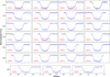 |
Fig. 1 Observations of 27 transits were conducted from 2015 to 2023 utilizing the DFOSC instrument on the Danish Telescope at La Silla Observatory. Transits that exhibit possible starspots are enclosed within rectangular markers. The observation dates follow the YY/MM/DD format. |
3.3 Literature data
WASP-19 b has been extensively observed and studied by various research teams over the years. We have collected an additional 43 complete transit light curves from previously published works: Hebb et al. 2010; Albrecht et al. 2012; Anderson et al. 2013; Tregloan-Reed et al. 2013; Hellier et al. 2011; Mancini et al. 2013; Lendl et al. 2013; Dragomir et al. 2011; Bean et al. 2013; Espinoza et al. 2019; Sedaghati et al. 2017; Patra et al. 2020; Sedaghati et al. 2015; Petrucci et al. 2020. These previously published observations will allow us to expand the temporal baseline of our investigation and provide crucial insights into the longterm evolution of the WASP-19 system. For mid-transit timing information, see Table A.2.
4 Light curve analysis
4.1 Starspot modeling and analysis
To model the influence of stellar activity on transit light curves, we used the PRISM (Planetary Retrospective Integrated Starspot Model) code2 (Tregloan-Reed et al. 2013). This tool enables the simultaneous modeling of planetary transits and potential starspot crossings by pixelating the stellar disk and simulating flux variations caused by occulted spots. PRISM is coupled with the GEMC (Genetic Evolution Markov Chain) optimization algorithm, which merges genetic algorithms with Markov chain Monte Carlo (MCMC) techniques. This hybrid framework performs global optimization in the first stage and then refines the best-fit parameters in a Bayesian context during the second stage via differential evolution Markov chain Monte Carlo (DEMC).
The modeling assumes a quadratic limb-darkening law and can accommodate circular or eccentric orbits. The photometric transit model is defined by the following key parameters: the sum of fractional radii (r* + rp), the ratio of radii (k = Rp/R* = rp/r*), the orbital inclination (i), the limb-darkening coefficients (u1, u2), and the mid-transit time (T0). Starspots are modeled with four additional parameters: the spot latitude and longitude (θ, φ), which are directly fitted, the angular radius (rspot), and the spot contrast (ρ), defined as the ratio of the surface brightness of the starspot to that of the surrounding photosphere.
We applied this modeling framework to the Danish telescope data, where several light curves exhibited anomalies consistent with spot-crossing events (see Fig. 2). For those events, we fit the light curves using PRISM+GEMC to characterize the spot properties. Similarly, where applicable, we analyzed TESS light curves and literature data (e.g., WASP-19: Tregloan-Reed et al. (2013); WASP-6: Tregloan-Reed et al. (2015); HAT-P-32: Tregloan-Reed et al. (2018); TESS light curves: Tregloan-Reed & Unda-Sanzana 2019, 2021) using the same approach.
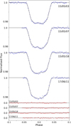 |
Fig. 2 Light curves of transits observed with the Danish telescope, with starspots modeled using PRISM+GEMC, along with the corresponding residuals. |
4.2 Reanalysis of literature light curve data for potential starspots
To ensure homogeneity in the analysis, previously published light curves from Lendl et al. (2013), Patra et al. (2020), and Petrucci et al. (2020) were reanalyzed using the PRISM+GEMC modeling framework. By reprocessing these observations with a uniform modeling approach, potential systematics arising from different reduction and modeling techniques in the literature are minimized, thereby enhancing the reliability and comparability of the derived parameters.
A comprehensive summary of the identified and modeled starspots, including their parameters and uncertainties, is presented in Table C.2. This table provides details on the starspot locations, radii, contrast ratios, and associated uncertainties, facilitating direct comparisons between different observational datasets and improving the robustness of our conclusions regarding the stellar variability in the WASP-19 system.
Combined photometric parameters for WASP-19 compared with previous studies.
4.3 Geometric and physical parameters results
Each light curve from the Danish telescope was modeled independently, along with transit light curves compiled from the literature (see Sect. 4.2). The TESS observations were treated separately, with the transits of WASP-19 extracted and fitted individually due to their high cadence and large number.
After individual modeling, the photometric parameters from all datasets were combined using a weighted mean approach to obtain final representative values for the system. These combined results provide robust constraints on the physical configuration of the WASP-19 system. The final photometric parameters, along with comparative values from previous studies, are presented in Table 1.
To derive the physical parameters of the WASP-19 system, we employed a model-independent method that does not rely on stellar evolutionary models such as MESA (Modules for Experiments in Stellar Astrophysics) or isochrone fitting. Instead, we used a direct estimate of the stellar radius based on the Infrared Flux Method IRFM (Blackwell & Shallis 1977), combined with Gaia DR3 parallaxes and broadband spectral energy distributions. This approach follows the methodology of Goswamy et al. (2024), who derived homogeneous radii for all WASP host stars.
This approach is particularly advantageous because it minimizes the systematic uncertainties and assumptions inherent in model-based techniques. For example, isochrone fitting typically requires prior knowledge of the star’s age, metallicity, and evolutionary state, factors that can bias the derived planetary parameters. In contrast, a model-independent method allows us to use purely geometric and dynamical constraints from the light curve and radial velocity data, leading to more robust and transparent results.
Adopting a stellar radius of  R⊙ from Goswamy et al. (2024), and following the procedure outlined in Morrell et al. (2026), we derived the complete set of stellar and planetary parameters and presented them in Table 2.
Physical parameters of the WASP-19 system.
5 Timing analysis
To measure the TTVs, we included all available transit light curves, both from this work and from previously published datasets, and reanalyzed them homogeneously using the PRISM+GEMC modeling framework. In total, 114 transit events were modeled to extract self-consistent mid-transit times, excluding any secondary eclipse (occultation) timings reported in the literature. The derived mid-transit times and their residuals for each of these events are listed in Table A.2.
5.1 Fitting the mid-transit timing data
To investigate the presence of orbital decay in the WASP-19 system, we fitted linear, quadratic, and cubic polynomial models to the residuals between the observed mid-transit times and those predicted by a constant-period ephemeris. Specifically, we first used best-fit linear ephemeris to compute expected transit times under the assumption of a strictly periodic, unperturbed orbit. The residuals, i.e., the differences between the observed and predicted transit times, were then modeled as a function of epoch number E using increasingly complex polynomial representations.
The linear model represents a constant orbital period and a fixed reference mid-transit time, which includes two free parameters (kF = 2)
 (1)
(1)
where T0 is the reference mid-transit time and P is the orbital period. The quadratic model represents a scenario in which the orbital period changes uniformly with time, introducing a constant period derivative. This form of evolution is the expected signature of tidal dissipation; however, other processes such as long-term apsidal precession, dynamical perturbations from an unseen companion, or secular variations induced by stellar magnetic activity cycles or the Applegate mechanism can produce comparable curvature in the timing residuals. This involves three free parameters (kF = 3)
 (2)
(2)
Finally, a cubic model was included, which extends the quadratic approach by allowing for an additional degree of freedom, representing variations in the rate of period change itself. It involves four free parameters (kF = 4), making it more flexible in capturing complex changes in the orbital period, such as higher-order effects due to tidal dissipation or interactions with other bodies (e.g., additional planets or stellar companions). A positive cubic term could suggest that the rate of orbital decay is slowing down or, conversely, accelerating, depending on its sign and magnitude.
Two widely employed statistical tools to compare models of diverse levels of complexity are the Akaike information criterion (AIC) and the Bayesian information criterion (BIC). These criteria balance the goodness of fit, quantified by the chi-squared statistic (χ2), against the complexity of the model, represented by the number of free parameters (kF).
The formulas for the AIC and BIC are defined as follows
 (3)
(3)
 (4)
(4)
where, χ2 is the chi-squared statistic representing the goodness of fit, kF is the number of free parameters in the model, NP is the number of data points.
The timing dataset is heterogeneous, combining transit times derived from multiple instruments and analyzes over a ∼15-year baseline. As a result, the formal timing uncertainties do not fully capture the observed scatter in the residuals, and the reduced χ2 values exceed unity for all the tested ephemeris models. Table 3, illustrated in Fig. 3, shows that the reduced χ2 decreases as the ephemeris becomes more complex; however, this behavior alone may simply reflect the increased flexibility of higher-order models rather than an unambiguous physical significance. To assess whether the inclusion of additional parameters is statistically justified, we therefore rely on AIC and BIC as relative model comparison metrics. The BIC evaluates which model is most strongly supported when penalizing complexity, while the AIC identifies the model that optimally balances goodness of fit and parsimony. Both criteria consistently favor cubic ephemeris over linear and quadratic alternatives when applied to the full dataset listed in Table A.2.
Physically, the cubic term captures a slow, non-periodic trend in the orbital evolution of WASP-19 b. Such behavior may reflect a low-order secular process, such as tidal dissipation or apsidal precession, that would not translate into a strictly periodic signal. The resulting curvature in the transit timing residuals thus provides compelling evidence of non-linear orbital evolution within the system (e.g., Maciejewski et al. 2018; Penev et al. 2018; Gomes et al. 2021; Yalçinkaya et al. 2024). This interpretation is consistent with theoretical expectations that tidal dissipation and apsidal motion in short-period hot-Jupiters induce secular, non-periodic drifts in transit timings rather than sinusoidal variations, producing the type of curvature captured by a cubic ephemeris. As discussed previously, other mechanisms can, in principle, also generate higher-order trends. In contrast to previous works (see, e.g., Petrucci et al. 2020) that favored a purely linear ephemeris and found no sign of decay, our bootstrap-based MCMC analysis (see below) supports the cubic model, suggesting that the planet’s orbit may be undergoing subtle, measurable changes consistent with long-term dynamical effects.
Model selection robustness against outliers. To evaluate whether the detected departure from constant-period timing variations is influenced by the heterogeneous quality of the dataset, we compared model performance for the complete sample (including TESS) and for a subset excluding TESS (see Appendix A). As expected from its higher photometric scatter, the inclusion of TESS increases the values of the overall χ2 and the information-criterion values. Nevertheless, in both cases, the cubic ephemeris remains consistently favored over the linear and quadratic models, indicating that the long-term curvature in the timing residuals is not driven by the lower-precision TESS points.
To further assess robustness against potentially influential measurements, we performed a series of complementary filtering tests. Removing the most uncertain transit times of 5 % produced only a minor reduction in scatter, while excluding points beyond 1σ or 2σ from the best-fitting trend yielded greater improvements in χ2, AIC, and BIC. In all instances, the cubic model continued to provide the lowest information-criterion scores, demonstrating that no single point or subset governs the inferred curvature.
Finally, we applied a random hold-out cross-validation procedure (Xval), in which 20% of the timings were removed randomly and the remaining 80% refitted over 104 iterations. Across all realizations, the cubic ephemeris delivered prediction errors with a median absolute deviation comparable to the simpler models while showing the smallest systematic bias. Although the reduced values χ2 remain greater than unity in these tests, reflecting the intrinsic heterogeneity of the timing dataset and the presence of excess scatter beyond the formal uncertainties quoted, this behavior is consistent between all tested models. The persistence of the cubic preference under cross-validation therefore indicates that the inferred non-linear trend is not an artifact of individual outliers or underestimated uncertainties, but a coherent long-term feature of the data. This confirms that the non-linear trend persists regardless of which measurements are withheld.
Comparison of linear, quadratic, and cubic ephemeris model for WASP-19b.
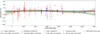 |
Fig. 3 Transit-timing residuals of WASP-19 b with respect to the best-fitting linear ephemeris. The red, blue, and purple points represent literature, Danish, and TESS data, respectively, with their associated timing uncertainties. The solid black, green, and brown curves correspond to the median fits from the linear, quadratic, and cubic polynomial models, respectively. Shaded regions indicate the 68 % confidence intervals derived from 20000 bootstrap realizations of each model’s MCMC posterior distribution. |
5.2 Tidal quality factor Q'*
Although tidal decay would, observationally, mean as a quadratic trend in transit timings, our model comparison shows that the quadratic ephemeris is not statistically preferred (see Sect. 5.1). To independently assess whether tidal decay could still be responsible for the observed deviations, we proceed to constrain the modified stellar tidal quality factor. The tidal quality factor (Q*) is a measure of the efficiency of the dissipation of tidal energy (Ogilvie 2014). To constrain Q*, we follow the approach outlined by Birkby et al. (2014), which describes the modified tidal quality factor as
 (5)
(5)
where k2 is the Love number (Love 1912). The modified tidal quality factor is related to measurable properties of the system through the equation
 (6)
(6)
where  , denoted as rA, represents the fractional radius of the star, and p1 is the quadratic coefficient in the ephemeris.
To estimate the tidal quality factor Q′*, one of the critical steps involves determining which model best fits the data: a model in which the orbital period remains constant or a model in which the orbital period changes (indicating potential orbital decay or perturbations). As said in Sect. 5.1, our data support the cubic ephemeris.
To quantify the extent of orbital decay indicated by the quadratic trend, we utilize the best-fit value of the quadratic term p 1 = −3.1536 × 10⁻¹¹ from Table 3. Although the cubic model yields a better statistical fit (AIC and BIC), the quadratic term directly captures the long-term, monotonic decrease in orbital period associated with tidal decay. However, because our full TTV analysis does not detect decay at this level, the decay rate inferred from the quadratic fit must be interpreted as an upper limit. Following the formulation from Birkby et al. (2014), the derived quadratic term provides a lower limit on the stellar modified tidal quality factor of Q'* ≈ 106.29±0.07. The uncertainty given reflects propagated errors in MA, Mp, and rA. This lower limit is consistent with previous constraints for the hot-Jupiters (e.g., Bonomo et al. 2017).
5.3 Further analysis and interpretation of TTV restricted to TESS data
While in the previous section we searched for TTVs across the entire 15-year dataset, here we refine our restricted analysis (Appendix B) by focusing on TESS-only light curves with 82 valid mid-transit times without the impact of starspots, which offer exceptional photometric precision, cadence uniformity, continuous temporal coverage, and less contamination from heterogeneous ground-based timing data.
For this purpose, we first derived individual TTVs from the TESS sectors using the allesfitter framework (Günther & Daylan 2019, 2021), which simultaneously models the transit light curve through a GP baseline model using MCMC to obtain statistically robust uncertainties. The measured TTVs were then compared with the synthetic TTV series computed with the N-body TTVFast (Deck et al. 2014) simulation. In this context, allesfitter provides the measured TTVs that consider all possible astrophysical effects (including gravitational perturbation, tidal dissipation, and potential apsidal motion), whereas TTVFast isolates the component of TTVs that arises purely from gravitational perturbations. The comparison between the measured TTVs and synthetic TTV series allows us to assess whether additional secular or dissipative effects are required to explain the observed transit timing residuals in Fig. 3.
The resulting TTVFast model for the TESS-only dataset is illustrated in Fig. 4. We chose to perform the TTV analysis exclusively on the TESS dataset because the TTVFast simulation imposes a hard limit of 5000 mid-transit times per run. Given the short orbital period of WASP-19 (≈0.79 days), this restricts the effective simulation window to ∼3950 days, which aligns with the TESS baseline but falls short of spanning the full 15-year ground-based dataset. Thus, using TESS alone enables a consistent and uninterrupted TTV analysis within this constraint. The agreement between the measured TTVs and synthetic TTV series is excellent, yielding a reduced chi-square of  and a p-value of 0.9993. The inferred TTV amplitude, ATTV = 1.102 × 10⁻⁶ min, suggests that the TTVs measured by allesfitter are consistent with the TTVFast model (Hughes & Hase 2010). No systematic trend or coherent deviation is detected across six TESS sectors, implying that WASP-19b is dynamically isolated and exhibits no measurable TTVs due to gravitational perturbations from additional companions.
To further explore the dynamical stability of an injected perturber in lower-order near mean-resonance with WASP-19 b, we plotted the mean exponential growth factor of nearby orbits (MEGNO; Cincotta & Simó 2000; Goździewski et al. 2001; Borkovits et al. 2003; Hinse et al. 2010) map through a grid search in the parameter space (P′/Pb, M′) ∈ ([0.1,9.9], [10−6 M⊕, 106 M⊕]) in Fig. 5 to analyze the orbit stability of an injected perturber at sites close to WASP-19b. The upper mass limit of the perturber is estimated by applying the TTV2Fast2Furious code3 (TTV2F2F; Hadden et al. 2019) to the TTVFast simulation. Under the assumption of a coplanar perturber in a circular orbit as the initial conditions, we start the numerical simulation in this putative three-body system by integrating each grid point from the initial conditions for 60 000 yr to fully saturate chaotic regions in the MEGNO map (Hinse et al. 2010). The MEGNO indicator 〈Y〉 is then computed and illustrated with color bars, where 〈Y〉 ≈ 2 indicates quasi-periodic (regular) dynamics and 〈Y〉 → 5 indicates chaotic (unstable) behavior. For candidates of the injected perturber in the 〈Y〉 ≈ 2 region, they are more likely to be recovered.
Our MEGNO map in Fig. 5 rules out the unstable region between the period ratio 2:3 and 3:2, which is consistent with the MEGNO map presented by Cortés-Zuleta et al. (2020). However, our map did not discover the evidence of 5:2 and 3:1 mean-motion resonances. This difference is probably because we derive the perturber’s upper mass limit from WASP-19b’s synthetic TTV series caused by gravitational perturbations, while Cortés-Zuleta et al. (2020) directly calculated the RMS statistics of original transit timing residuals containing all astrophysical effects in the O-C plot.
After combining the MEGNO indicators on our map in Fig. 5 with the RV constraints in the region where P′ < 20 d (Bernabò et al. 2024), it turns out that only near 1:2 and near 2:1 resonances with an upper mass limit ∼10 M⊕ are possible for a stable near-resonant perturber. However, since Bernabò et al. (2024) have already excluded the P′ < 20 d region through a χ2 analysis by injecting a perturber to their simulation, we do not prefer the existence of a lower-order near-resonant perturber.
For a higher-order near resonant exterior perturber, when we are using the TTV2F2F code to derive its mass-eccentricity constraints, the contour plot is not very constraining, revealing that there is no strong evidence of the existence of an unseen perturber in the WASP-19 system. Therefore, we conclude that the more favorable cubic model with a smaller  cannot be attributed to an unseen perturber.
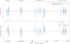 |
Fig. 4 Measured TTVs derived from allesfitter when modeling TESS observations for WASP-19 b in the upper plot with their residuals illustrated in the lower plot. The TTVFast model yields a negligible TTV amplitude of ATTV = 1.102 × 10⁻⁶ min. |
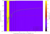 |
Fig. 5 MEGNO stability map depicting the upper mass limit (within ±1σ (68.3%), ±2σ (95.4%), and ±3σ (99.7%) confidence intervals) of an injected hypothetical perturber in the WASP-19 system. The red horizontal dashed lines represent the perturber’s mass range between M = 400 M⊕ and M = 1.4 M⊕ determined from the RV constraints (Bernabò et al. 2024). The red vertical dashed lines from left to right represent the perturber’s unstable orbits in 2:3, 1:1, and 3:2 resonances with WASP-19b determined in this paper, while the black vertical dashed lines from left to right represent the perturber’s stable orbits in 1:2, 5:3, 2:1, 5:2, and 3:1 resonances with WASP-19b found by Cortés-Zuleta et al. (2020). |
5.4 Constraints on apsidal precession and internal structure of WASP-19b
To further test the hypothesis that long-term deviations from a linear ephemeris are driven by apsidal precession, we applied the classical precession model described in Ragozzine & Wolf (2009). We modeled the observed mid-transit times using the following expression for an apsidally precessing system
 (7)
(7)
where T0 is the reference transit time, Ps is the sidereal period, e is the orbital eccentricity, ω0 is the argument of the periastron at epoch zero, and ω̇ is the apsidal precession rate in radians per orbit. We fixed the eccentricity at e = 0.00172, following the analysis of Bernabò et al. (2024), who derived this value from the combined RV and photometric constraints.
Using non-linear least squares optimization, we fit this model to our compiled transit mid-times, which span over 15 years. The resulting best-fit apsidal precession rate was ω̇obs = (1.00 ± 0.12) × 10−4 rad/orbit.
To interpret this observationally derived value, we computed the expected contribution from general relativity using the equation below, and by substituting the system parameters, we found
 (8)
(8)
Subtracting this from the total observed rate yields the tidal component of the precession
 (9)
(9)
The planetary Love number k2p, which characterizes the planet’s interior response to tidal forces, can then be derived using
 (10)
(10)
Rearranging, we solved for k2p
 (11)
(11)
This value agrees well with the result of Bernabò et al. (2024), who reported  based on a joint analysis of transits, occultations, and radial velocity data (see their Sect. 6.1). Nevertheless, the two estimates are consistent within 2σ and reinforce the interpretation that WASP-19b experiences an observable apsidal precession due to tidal distortion.
Combined with the statistical evidence of a cubic ephemeris (see Sect. 5.1), this dynamical modeling reinforces the view that the long-term orbital evolution of WASP-19b is not driven by orbital decay, but by apsidal motion resulting from both internal planetary structure and possible secular forcing from a wide-orbit stellar companion identified in Bernabò et al. (2024).
6 Transmission spectrum analysis
WASP-19b has been extensively studied by several researchers (e.g., Mancini et al. 2013; Mandell et al. 2013; Sedaghati et al. 2015). However, only a few have taken stellar anomalies into account, which can significantly impact the accuracy of the results. By modeling and correcting our data homogeneously for the effects of starspots and other stellar activity in the light curve, we can substantially improve the precision of the measured planet-to-star radius ratio, with uncertainties reduced by up to a factor of two compared to earlier studies. For example, we report a refined value of Rp∕R* = 0.1415 ± 0.0014, compared to previously published uncertainties ranging from ±0.002 to ±0.006 (e.g., H10, AL12, P20; see our Table 1). Such precision is crucial when interpreting atmospheric absorption features in transmission spectra, especially in hot-Jupiters like WASP-19 b, where stellar activity is known to distort transit depths (Rackham et al. 2018; Oshagh et al. 2014). In our analysis of WASP-19b, we incorporated starspot modeling into the light curve fitting process. This approach allowed us to refine the transit depth measurements, enhancing our ability to detect subtle atmospheric absorption features. Correcting for stellar activity not only reduces systematic errors, but also increases sensitivity to important atmospheric signals, such as molecular absorption bands, which may otherwise be obscured by noise.
6.1 Photometric spectrum
In our study of WASP-19b, a strongly irradiated hot-Jupiter, we used photometric data to reconstruct a low-resolution photometric transmission spectrum. Since our objective was closely tied to the orbital decay study, we did not incorporate occultation data, which would otherwise be necessary to characterize the planet’s dayside emission. Although such data can complement atmospheric characterization, especially for retrieving temperature profiles and detecting thermal inversions, their inclusion is not critical for probing transmission features, which are dominated by the planetary limb. Instead, we focused exclusively on transit observations to enhance the reliability of our constraints on orbital precession and the transmission spectrum derived purely from primary transits. We employed light curves obtained from the Danish telescope in the R and I filters, TESS in the R filter, along with multi-wavelength light curves from the literature across different passbands (g, J, H, K). These light curves allowed us to investigate the atmospheric characteristics on the nightside of WASP-19b. To ensure the accuracy of our analysis, we excluded incomplete or unreliable light curves, as discussed in Sect. 3.1, and focused solely on complete datasets. Using the PRISM+GEMC algorithm, we analyzed each light curve to compute the planet-to-star radius ratio (Rp/R*) for each passband. During this process, we kept other photometric parameters constant, using the best-fitting values determined from the overall light-curve fitting. This method ensured that any observed variations in the radius ratio were genuine and not influenced by systematic errors or instrumental effects.
For each of the six passbands, we calculated the Rp/R* values and then computed a weighted mean for each passband to increase the precision of our estimates. These weighted averages formed the basis for our reconstructed photometric transmission spectrum. Although this multi-wavelength photometry is lower in resolution than traditional transmission spectroscopy, it provides valuable insight into the composition of WASP-19 b’s nightside atmosphere.
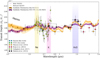 |
Fig. 6 Variation of the planetary radius, expressed as transit depth, as a function of wavelength. Sky-blue points correspond to Danish-DFOSC (this work), lime to TESS (this work), orange to GROND (Mancini et al. 2013), crimson to MMIRS (Bean et al. 2013), green to Sedaghati et al. (2015), and black to Huitson et al. (2013). Vertical error bars represent measurement uncertainties, while horizontal bars indicate the full width half maximum (FWHM) of the respective passbands. Synthetic photometric points were computed using the SVO SpecPhot tool to obtain flux-weighted transit depths at the effective wavelengths of the UV-optical filters. Retrievals were performed with POSEIDON including the opacities of Na, K, TiO, VO, and H2O. The orange curve shows the median best-fit model excluding TiO and VO, with 1σ and 2σ confidence intervals. The purple curve shows the median best-fit model including TiO and VO, with corresponding uncertainties. See Sect. 6.2 for details. |
6.2 Variation of planetary radius with the wavelength
To ensure a consistent transmission spectrum across heterogeneous datasets, we applied small additive transit-depth offsets to each instrument, derived by aligning all measurements with the high-S/N Hubble Space Telescope (HST) STIS+WFC3 baseline (Huitson et al. 2013) through weighted interpolation and bootstrap-estimated uncertainties with final offset values listed in Table C.1 (see Appendix C for full details of the baseline correction procedure).
Figure 6 shows the variation of k as a function of wavelength, obtained from multiple datasets, including Danish-DFOSC instrument (R and I band), TESS space telescope (R band), GROND instrument covering multiple bands (Sloan g′, Sloan r′, Sloan i′, J, H, K) from Mancini et al. (2013) and MMIRS instrument (J, H, K bands) from Bean et al. (2013). Additionally, spectroscopic data points from Sedaghati et al. (2015) and Huitson et al. (2013) were included to increase the accuracy of the model. These datasets are compared against two atmospheric retrieval models, one that includes metal oxides: titanium oxide (TiO) and vanadium oxide (VO), and another that excludes these species.
Retrievals were performed using POSEIDON (MacDonald 2023; MacDonald & Madhusudhan 2017), a Bayesian atmospheric retrieval framework with 2000 live points. Best-fit retrieval assuming opacity sources from Na, K, and H2O, excluding TiO/VO (Orange line) predominately explains the observed spectrum of sodium (Na) at ∼0.59 Mm, potassium (K) at ∼0.77 Mm, water vapor (H2O) at ∼1.4 Mm, and Rayleigh scattering at blue optical wavelength in the He - H2 dominated atmosphere. Given the extreme irradiation of WASP-19b, the presence of metal oxides such as titanium oxide (TiO) and vanadium oxide (VO) is also anticipated. The best-fit incorporating TiO and VO opacities in the above spectrum are shown as the purple line. Metal oxides contribute significantly to atmospheric opacities, leading to stronger absorption features in the UV-optical wavelength (∼0.4-1.0 Mm).
The updated retrieval analysis based on the offset-corrected transmission spectrum further strengthens the statistical preference for an atmosphere without TiO/VO. The TiO/VO-free model yields a higher Bayesian evidence of ln Z = 354.29 ± 0.19, compared to ln Z = 350.37 ± 0.22 for the model including TiO and VO. This difference (∆ ln Z ≃ 4) represents strong statistical support for the TiO/VO-free scenario. In addition, the reduced chi-squared value improves significantly: the TiO/VO-free model achieves  (with χ2 = 96.17 for 52 degrees of freedom), whereas the model including TiO/VO yields a slightly poorer fit with
  . These improvements, which are substantially better than our previous pre-offset results (
 ), demonstrate that homogenizing the heterogeneous datasets through offset correction reduces inter-instrument discontinuities and prevents spurious spectral gradients from being misinterpreted as TiO/VO absorption. Consequently, the offset-corrected retrieval provides a more coherent and physically consistent interpretation of the planetary atmosphere, favoring the presence of Na, K, H2O, and Rayleigh scattering, while offering less compelling statistical evidence of TiO/VO in the transmission spectrum of WASP-19b.
However, previous high-resolution spectroscopic studies, such as Sedaghati et al. (2017) using VLT-FORS2, reported a tentative detection of TiO features in the transmission spectrum of WASP-19 b. This discrepancy likely arises due to the difference in the spectral resolution and analysis approach. Sedaghati et al., employed differential spectroscopy using FORS2, which provides significantly higher spectral resolution and is capable of isolating narrowband features such as TiO absorption bands in the optical range. In contrast, the photometric transmission spectrum used in our study, though covering a wide wavelength range, relies on broadband photometry with limited spectral resolution.
Such photometric data tend to dilute or smooth out narrow spectral features, making it challenging to resolve molecular opacities like TiO/VO, particularly in the presence of instrumental systematics or stellar heterogeneities. Although we incorporated the spectroscopic data from Sedaghati et al. (2015) into our combined spectrum, the retrieval model still favors a solution without TiO/VO. This likely reflects the dominant influence of the lower-resolution photometric datasets included in the analysis. In addition, to complement the photometric dataset, synthetic photometric points were generated using the SVO SpecPhot4 tool by uploading the retrieved model spectra of WASP-19b (spanning 0.3-2.5,Mm) and integrating them into UV-optical filters: Rosetta/OSIRIS_WAC.F71, F81, UV375, HST/ACS_HRC.F435W, and F475W to obtain flux-weighted transit depths at the corresponding effective wavelengths. These synthetic points (plotted as colored squares in Fig. 6) represent where future or existing photometric observations would probe each model retrieved. They serve to extend the model predictions into wavelength regions with limited observational coverage, providing a continuous theoretical reference that highlights the expected spectral behavior of both the TiO/VO-included and TiO/VO-free retrievals.
Overall, our result does not refute the possibility of TiO/VO in WASP-19 b’s atmosphere, but rather highlights the limitations of broadband photometry in confidently detecting such species. High-resolution, spectrally resolved follow-up observations are essential to confirm the presence and abundance of metal oxides. Although our retrieval analysis does not provide strong evidence of the presence of TiO/VO, it is important to consider that atmospheric composition may not be static. Beyond observational limitations, the dynamical evolution of the planet’s orbit itself can significantly affect atmospheric structure and chemistry (Komacek & Showman 2020; May & Rauscher 2021). In hot-Jupiter systems like WASP-19b, while orbital decay due to tidal dissipation is a widely expected phenomenon, other processes such as apsidal precession may play an equally critical role.
In the case of WASP-19b, the presence of apsidal precession is suggested by the cubic trend observed in the transit timing residuals (see Sect. 5.1). This kind of orbital evolution is not only of dynamical interest, but it can also lead to periodic changes in the stellar irradiation received by the planet (Langton & Laughlin 2008; Rauscher & Kempton 2014). These fluctuations can result in time-variable atmospheric temperatures, which in turn influence molecular abundances through changes in chemical equilibrium. Consequently, absorbers such as H2O, TiO, and VO may experience redistribution or dissociation over time, leading to variations in the observed transmission spectrum.
7 Results
This study provides a comprehensive analysis of the TTVs and atmospheric properties of the ultra-short-period hot-Jupiter, WASP-19b. Our main results are as follows:
Using an extensive dataset spanning more than a decade, we modeled the transit timings of WASP-19 b with linear, quadratic, and cubic ephemeris models to assess potential departures from a constant-period orbit. due to the heterogeneous quality of the timing measurements, the reduced values χ2 exceed unity for all tested ephemerides. Nevertheless, a relative model comparison using the AIC and BIC consistently favors cubic ephemeris over linear and quadratic models (see Table 3). In a purely mathematical sense, the cubic term represents slow, non-periodic curvature in the observed-minus-calculated (O-C) diagram. Physically, such curvature may arise from low-order secular processes, including tidal dissipation or apsidal precession, rather than from periodic perturbations by additional planets. However, given the modest amplitude of the observed deviations (∼50-100 s) relative to the general scatter in the timing data, the current dataset does not provide statistically significant evidence of genuine TTVs. The cubic ephemeris should therefore be interpreted as an empirical description of a long-term trend rather than as a definitive proof of ongoing dynamical perturbations. This conclusion is consistent with theoretical expectations that tidal or pre-cessional effects in short-period systems may produce smooth, low-amplitude drifts over multi-year baselines (e.g., Maciejewski et al. 2018; Penev et al. 2018; Gomes et al. 2021; Yalçinkaya et al. 2024), which can only be robustly confirmed through future high-precision monitoring.
To verify the robustness of the timing signal, we performed a dedicated analysis using only the six available TESS sectors. Individual TTV were derived using allesfitter (Günther & Daylan 2019, 2021), and compared with synthetic TTV series from the N-body simulation TTVFast (Deck et al. 2014). In this framework, allesfitter provides the observed transit timing residuals (including all astrophysical effects), while TTVFast isolates the component of TTVs produced purely by gravitational perturbations. The resulting fit (Fig. 4) shows an excellent agreement between the observed TTV and modeled TTV series (
 , p-value = 0.9993), with a negligible amplitude of ATTV = 1.102 × 10⁻⁶ min. No coherent trend or periodicity is detected across the TESS dataset, indicating that WASP-19 b’s orbit is dynamically stable and that any potential perturbations are below the current detection threshold.
Given the absence of measurable TTVs, we explored whether a perturber capable of inducing the observed low-amplitude curvature could exist within dynamically stable regions. Using MEGNO maps and the TTV2F2F code (Hadden et al. 2019), we scanned the parameter space (P′/Pb, M′) ∈ ([0.1,9.9], [10−6,106] M⊕) and found that all near-resonant solutions with P′ < 20 d and M′ > 10 M⊕ are dynamically unstable or are ruled out by radial velocity limits. The remaining stable parameter space corresponds to perturbers below ∼10 M⊕ near the 1:2 and 2:1 resonances, but these would produce TTV amplitudes well below the current detection sensitivity.
The observed curvature in the long-term dataset is best explained by a slow secular process, such as apsidal precession or weak tidal dissipation, rather than by an external perturber. Modeling the transit times with a precession term yields a rate of ω̇obs = (1.00 ± 0.12) × 10−4 rad orbit−1 and an associated Love number k2p = 0.107 ± 0.08, in agreement with Bernabò et al. (2024). The presence of the wide stellar companion WASP-19 B could further sustain the slight eccentricity required for ongoing precession through Kozai-Lidov oscillations.
To assess robustness, we repeated the analysis on reduced subsets of the timing data after excluding the highest-uncertainty points (top 20-40%). In all cases, the cubic model remained marginally favored, but the absolute χ2 values remained > 1 and the residual scatter showed minimal improvement. This confirms that the statistical preference for a cubic fit arises primarily from the shape of the residual distribution rather than from genuine dynamical effects. The observed r.m.s. scatter of 46-50 s still exceeds the level required to detect secular orbital decay (∼10s over a decade), highlighting the need for future high-precision timing campaigns.
Our photometric transmission spectrum of WASP-19b shows no statistically significant evidence of TiO/VO absorption. After applying per-dataset offset corrections, the TiO/VO-free retrieval model yields a substantially higher Bayesian evidence (ln Z = 354.29 ± 0.19) and a lower reduced chi-square (
 ). This improvement over our pre-offset analysis (
 ) demonstrates that homogenizing the datasets leads to a more physically consistent interpretation. The preference for a TiO/VO-free atmosphere contrasts with previous high-resolution FORS2 detections (Sedaghati et al. 2017), a discrepancy most likely arising from the inherently lower spectral resolution of broadband photometry, which tends to smooth out narrow molecular features. If apsidal precession modulates irradiation over time, it could in principle lead to small-scale variability in the atmospheric temperature structure.
In summary, our analysis statistically favors the cubic ephemeris model for WASP-19b, indicating measurable curvature in the long-term transit timing data. The most consistent physical interpretation of this trend is the apsidal precession of a slightly eccentric orbit, possibly sustained by long-term gravitational perturbations from the stellar companion WASP-19 B. Although the observed amplitude remains small relative to measurement uncertainties, the persistent preference for a non-linear model across independent datasets suggests that secular orbital evolution rather than tidal decay or stochastic noise is currently shaping the long-term behavior of WASP-19 b.
8 Discussion
The orbital and atmospheric properties of WASP-19 b have been extensively explored since its discovery, with numerous efforts focusing on detecting signs of orbital decay and probing its atmospheric composition (Hebb et al. 2010; Mancini et al. 2013; Sedaghati et al. 2017; Patra et al. 2020). Our comprehensive reanalysis of more than 15 years of transit observations reveals a statistically significant curvature in the transit timing residuals, favoring a cubic ephemeris model. This curvature, combined with the moderate period-change rate derived from our fits, provides evidence that WASP-19 b might be undergoing a long-term dynamical evolution dominated by apsidal precession rather than rapid tidal decay.
Our updated analysis yields a period change rate of Ṗ = −0.99 ± 0.20 ms yr−1 (Table A.1), which places our result in close agreement with the value reported by Biswas et al. (2025, Ṗ = −1.1 ± 0.4 ms yr−1) and within the same order of magnitude as the upper bound derived by Rosério & et al. (2022, −1.40 ± 0.88 ms yr−1). Our measured Ṗ is notably smaller than the earlier claim of rapid orbital decay reported by Patra et al. (2020, Ṗ = −6.50 ± 1.33 ms yr−1 ) and slightly larger than the near-constant period solution of Ma et al. (2025). This intermediate value, together with the superior statistical performance of the cubic ephemeris, suggests that the orbital evolution of WASP-19b is best explained by a slow secular process such as apsidal precession rather than monotonic tidal decay.
The cubic term encapsulates the non-linear curvature expected from precessional motion of a slightly eccentric orbit. The direct fitting of a precession model to the dataset yields a precession rate of (1.00 ± 0.12)×10−4 rad orbit−1 corresponding to a planetary Love number of 0.107 ± 0.08, which aligns closely with the value of  reported by Bernabò et al. (2024). The consistency of these parameters across independent analyzes reinforces the interpretation that apsidal precession dominates the long-term timing evolution of WASP-19b. The wide-separation stellar companion WASP-19B may play a key dynamical role, inducing Kozai-Lidov oscillations or long-term secular forcing that sustain the small but nonzero eccentricity required for continued precession. Such secular interactions could also modulate the irradiation geometry of the planet over time, producing subtle variations in the structure and circulation of atmospheric temperature.
Although the cubic model is statistically favored (lowest AIC and BIC), the reduced values χ2 exceeding unity indicate that the timing dataset contains excess scatter beyond the formal uncertainties quoted. We recognize that this scatter is dominated by a subset of archival transit timings, particularly from older groundbased observations, for which the reported uncertainties may be underestimated. To mitigate this, we performed subset analyzes excluding high-uncertainty points (top 20-40%) and found that the cubic preference persisted, demonstrating that the inferred curvature is not driven by a small number of outliers or poorly constrained measurements. Moreover, the dedicated TESS-only analysis using allesfitter (Günther & Daylan 2019, 2021) and TTVFast (Deck et al. 2014) produced an excellent fit with negligible TTV amplitudes, indicating that short-period dynamical perturbations are not required to explain the data. This supports the interpretation that the long-term cubic trend reflects secular orbital evolution rather than stochastic noise or periodic forcing by an additional planet. Although we cannot entirely exclude the possibility of a low-mass external perturber, our MEGNO stability maps rule out companions more massive than ∼10 M⊕ near low-order resonances, thereby strengthening apsidal precession as the self-consistent physical explanation under the current observational constraints.
We note that occultation timings were intentionally excluded from this analysis due to their heterogeneous origins and instrument-dependent systematics. Restricting the analysis to homogeneously reduced transit timings ensures internal consistency over the 15-year baseline. Future observations combining precise secondary eclipse timings or phase-curve monitoring could further constrain eccentricity evolution and help discriminate between tidal and precessional contributions to the observed trend.
On the atmospheric side, the nature of the optical absorbers of WASP-19b has long been debated. With the offset-corrected transmission spectrum, our retrieval analysis strongly favors a model without TiO/VO, yielding a higher Bayesian evidence and a lower reduced chi-square compared to the TiO/VO-included model. This statistically robust preference for a TiO/VO-free atmosphere contrasts with the tentative TiO detection reported by high-resolution VLT-FORS2 spectroscopy by Sedaghati et al. (2017). The discrepancy likely arises from fundamental differences in spectral resolution: broadband photometric transmission spectra smooth over narrow TiO/VO bandheads that high-resolution differential spectroscopy can isolate. Additionally, TiO and VO are expected to be much more abundant and radiatively active on the intensely irradiated dayside of hot-Jupiters, where temperatures are higher and thermal dissociation or cold-trapping are less efficient (Fortney et al. 2008; Parmentier et al. 2018). Because our analysis relies exclusively on transmission (terminator) measurements and does not include occultation (dayside emission) data, any TiO/VO present primarily on the dayside may remain undetectable in the limb spectrum. High-altitude haze and clouds at the terminator (Sing et al. 2016) may further obscure metal oxide features. Instead, our retrieval consistently identifies Na, K, H2O, and Rayleigh scattering as the dominant opacity sources results consistent with earlier low-resolution photometric analyzes (Mancini et al. 2013) and physically plausible given the extreme irradiation of WASP-19b's environment.
A critical aspect in transmission spectroscopy is the impact of stellar activity, as uncorrected stellar variability can introduce systematic biases in transit depth measurements. Starspots, faculae, and flares have been known to distort transit light curves, leading to incorrect interpretations of planetary spectral features (Ioannidis et al. 2016). Our study accounts for these effects by incorporating PRISM+GEMC starspot modeling, which has been used successfully in prior exoplanet studies (Tregloan-Reed et al. 2013; Mancini et al. 2013). By correcting for stellar contamination, our modeling ensures that either the transit timing measurements or the retrieved planetary transmission spectrum is not significantly biased by stellar inhomogeneities, reinforcing the robustness of our results.
9 Conclusions
Our study provides supporting evidence that the long-term orbital evolution of WASP-19b could be dominated by the apsidal precession of a slightly eccentric orbit rather than rapid orbital decay. The statistically preferred cubic ephemeris, consistent precession rate, and derived Love number together point to a stable yet dynamically evolving system, possibly influenced by the distant stellar companion WASP-19B. On the atmospheric side, our analysis supports a TiO/VO-free composition with prominent Na, K, and H2O features and potential Rayleigh scattering. By combining a dynamically consistent ephemeris model with robust retrievals corrected for stellar activity, this work presents a coherent picture of WASP-19b as a hot-Jupiter whose orbital and atmospheric evolution are shaped primarily by long-term secular processes rather than by ongoing tidal decay. Looking ahead, the ability to distinguish between apsidal-precession and tidal-decay scenarios will critically depend on the availability of long-baseline high-quality transit timing data and on theoretical predictions of future transit times under both evolutionary pathways. While such forward modeling lies beyond the scope of the present work, the refined ephemeris and precession constraints reported here provide a robust empirical reference against which future, higher-precision measurements can be compared. As next-generation facilities such as JWST, PLATO, and the ELT achieve timing precisions at or below the ten-second level with improved control of systematics, WASP-19 b will become a benchmark system for probing long-term orbital evolution in hot-Jupiters and for assessing the role of data quality in detecting subtle secular effects.
Acknowledgements
We thank the anonymous referee and the editor for their constructive comments and valuable suggestions, which have significantly improved this manuscript. A.R.R acknowledges support from ANID Doctoral Scholarship program grant no. 21231937. A.B acknowledges support from the Deutsche Forschungsgemeinschaft (DFG, German Research Foundation) under Germany’s Excellence Strategy - EXC 2094 - 390783311. J.S acknowledges support from STFC under grant number ST/Y002563/1. F.A, M.A, and U.G.J acknowledge funding from the Novo Nordisk Foundation Interdisciplinary Synergy Programme grant no. NNF19OC0057374. T.C.H acknowledges funding from the Europlanet 2024 Research Infrastructure (RI) programme. The Europlanet 2024 RI provides free access to the world’s largest collection of planetary simulation and analysis facilities, data services and tools, a ground-based observational network and programme of community support activities. Europlanet 2024 RI has received funding from the European Union’s Horizon 2020 research and innovation programme under grant agreement No. 871149. R.F.J. acknowledges the support provided by the GEMINI/ANID project under grant number 32240028, by ANID’s Millennium Science Initiative through grant ICN12_009, awarded to the Millennium Institute of Astrophysics (MAS), and by ANID’s Basal project FB210003. E.K is supported by the National Research Foundation of Korea 2021M3F7A1082056. The following internet-based resources were used in research for this paper: exoplanet Transit Database (ETD); the SIM-BAD database; NASA’s Astrophysics Data System (ADS) Bibliograpic Services; We greatfully acknowledge the valuable suggestions and insightful discussions by Carlos Ferreria Lopez and Barbara Rojas, during the preparation of this manuscript.
References
- Albrecht, S., Winn, J. N., Johnson, J. A., et al. 2012, ApJ, 757, 18 [NASA ADS] [CrossRef] [Google Scholar]
- Anderson, D. R., Smith, A. M. S., Madhusudhan, N., et al. 2013, MNRAS, 430, 3422 [NASA ADS] [CrossRef] [Google Scholar]
- Antoniciello, G., Borsato, L., Lacedelli, G., et al. 2021, MNRAS, 505, 1567 [CrossRef] [Google Scholar]
- Ballard, S., Fabrycky, D., Fressin, F., et al. 2011, ApJ, 743, 200 [NASA ADS] [CrossRef] [Google Scholar]
- Barker, A. J., Braviner, H. J., & Ogilvie, G. I. 2016, MNRAS, 459, 924 [Google Scholar]
- Bastürk, Ö., Kutluay, A. C., Barker, A., et al. 2025, MNRAS, 541, 714 [Google Scholar]
- Bean, J. L., Désert, J.-M., Seifahrt, A., et al. 2013, ApJ, 771, 108 [NASA ADS] [CrossRef] [Google Scholar]
- Bernabò, L. M., Csizmadia, S., Smith, A. M. S., et al. 2024, A&A, 684, A78 [NASA ADS] [CrossRef] [EDP Sciences] [Google Scholar]
- Birkby, J. L., Cappetta, M., Cruz, P., et al. 2014, MNRAS, 440, 1470 [NASA ADS] [CrossRef] [Google Scholar]
- Biswas, S., Jiang, I.-G., Yeh, L.-C., et al. 2025, AJ, 170, 133 [Google Scholar]
- Bitsch, B., Lambrechts, M., & Johansen, A. 2015, A&A, 582, A112 [NASA ADS] [CrossRef] [EDP Sciences] [Google Scholar]
- Blackwell, D. E., & Shallis, M. J. 1977, MNRAS, 180, 177 [NASA ADS] [CrossRef] [Google Scholar]
- Bonomo, A. S., Desidera, S., Benatti, S., et al. 2017, A&A, 602, A107 [NASA ADS] [CrossRef] [EDP Sciences] [Google Scholar]
- Borkovits, T., Érdi, B., Forgács-Dajka, E., & Kovács, T. 2003, A&A, 398, 1091 [NASA ADS] [CrossRef] [EDP Sciences] [Google Scholar]
- Boss, A. P. 1997, Science, 276, 1836 [Google Scholar]
- Chatterjee, S., Ford, E. B., Matsumura, S., & Rasio, F. A. 2008, ApJ, 686, 580 [NASA ADS] [CrossRef] [Google Scholar]
- Cincotta, P. M., & Simó, C. 2000, A&AS, 147, 205 [NASA ADS] [Google Scholar]
- Cortés-Zuleta, P., Rojo, P., Wang, S., et al. 2020, A&A, 636, A98 [NASA ADS] [CrossRef] [EDP Sciences] [Google Scholar]
- Dawson, R. I. 2014, ApJ, 790, L31 [NASA ADS] [CrossRef] [Google Scholar]
- Deck, K. M., Agol, E., Holman, M. J., & Nesvornÿ, D. 2014, ApJ, 787, 132 [CrossRef] [Google Scholar]
- Doyle, A. P., Davies, G. R., Smalley, B., Chaplin, W. J., & Elsworth, Y. 2014, MNRAS, 444, 3592 [Google Scholar]
- Dragomir, D., Kane, S. R., Pilyavsky, G., et al. 2011, AJ, 142, 115 [NASA ADS] [CrossRef] [Google Scholar]
- Espinoza, N., Rackham, B. V., Jordán, A., et al. 2019, MNRAS, 482, 2065 [Google Scholar]
- Foreman-Mackey, D. 2016, J. Open Source Softw., 1, 24 [Google Scholar]
- Foreman-Mackey, D., Hogg, D. W., Lang, D., & Goodman, J. 2013, PASP, 125, 306 [Google Scholar]
- Fortney, J. J., Lodders, K., Marley, M. S., & Freedman, R. S. 2008, ApJ, 678, 1419 [CrossRef] [Google Scholar]
- Gallet, F., Bolmont, E., Mathis, S., Charbonnel, C., & Amard, L. 2017, A&A, 604, A112 [NASA ADS] [CrossRef] [EDP Sciences] [Google Scholar]
- Gomes, D. S., Ferreira, J. M., Ferreira, F., & Correia, A. C. M. 2021, A&A, 650, A178 [NASA ADS] [CrossRef] [EDP Sciences] [Google Scholar]
- Goswamy, T., Collier Cameron, A., & Wilson, T. G. 2024, MNRAS, 534, 843 [Google Scholar]
- Goździewski, K., Bois, E., Maciejewski, A. J., & Kiseleva-Eggleton, L. 2001, A&A, 378, 569 [NASA ADS] [CrossRef] [EDP Sciences] [Google Scholar]
- Gu, P.-G., Lin, D. N. C., & Bodenheimer, P. H. 2003, ApJ, 588, 509 [NASA ADS] [CrossRef] [Google Scholar]
- Günther, M. N., & Daylan, T. 2019, Allesfitter: Flexible Star and Exoplanet Inference From Photometry and Radial Velocity, Astrophysics Source Code Library [Google Scholar]
- Günther, M. N., & Daylan, T. 2021, ApJS, 254, 13 [CrossRef] [Google Scholar]
- Hadden, S., Barclay, T., Payne, M. J., & Holman, M. J. 2019, AJ, 158, 146 [NASA ADS] [CrossRef] [Google Scholar]
- Hadden, S., & Lithwick, Y. 2016, ApJ, 828, 44 [NASA ADS] [CrossRef] [Google Scholar]
- Hadden, S., & Lithwick, Y. 2017, AJ, 154, 5 [Google Scholar]
- Haisch, K. E. J., Lada, E. A., & Lada, C. J. 2001, ApJ, 553, L153 [NASA ADS] [CrossRef] [Google Scholar]
- Hebb, L., Collier-Cameron, A., Triaud, A. H. M. J., et al. 2010, ApJ, 708, 224 [NASA ADS] [CrossRef] [Google Scholar]
- Hellier, C., Anderson, D. R., Collier-Cameron, A., et al. 2011, ApJ, 730, L31 [NASA ADS] [CrossRef] [Google Scholar]
- Hinse, T. C., Christou, A. A., Alvarellos, J. L. A., & Gozdziewski, K. 2010, MNRAS, 404, 837 [NASA ADS] [CrossRef] [Google Scholar]
- Holczer, T., Mazeh, T., Nachmani, G., et al. 2016, ApJS, 225, 9 [Google Scholar]
- Hou, Q., & Wei, X. 2022, MNRAS, 511, 3133 [NASA ADS] [CrossRef] [Google Scholar]
- Hughes, I. G., & Hase, T. P. A. 2010, Measurements and their Uncertainties (New York: Oxford University Press) [Google Scholar]
- Huitson, C. M., Sing, D. K., Pont, F., et al. 2013, MNRAS, 434, 3252 [NASA ADS] [CrossRef] [Google Scholar]
- Ioannidis, P., Huber, K. F., & Schmitt, J. H. M. M. 2016, A&A, 585, A72 [NASA ADS] [CrossRef] [EDP Sciences] [Google Scholar]
- Jenkins, J. M., Twicken, J. D., McCauliff, S., et al. 2016, in Software and Cyberinfrastructure for Astronomy IV, 9913, SPIE, 1232 [Google Scholar]
- Komacek, T. D., & Showman, A. P. 2016, ApJ, 821, 16 [CrossRef] [Google Scholar]
- Komacek, T. D., & Showman, A. P. 2020, ApJ, 888, 2 [Google Scholar]
- Lambrechts, M., & Johansen, A. 2014, A&A, 572, A107 [NASA ADS] [CrossRef] [EDP Sciences] [Google Scholar]
- Langton, J., & Laughlin, G. 2008, ApJ, 674, 1106 [Google Scholar]
- Lendl, M., Gillon, M., Queloz, D., et al. 2013, A&A, 552, A2 [NASA ADS] [CrossRef] [EDP Sciences] [Google Scholar]
- Levrard, B., Winisdoerffer, C., & Chabrier, G. 2009, ApJ, 692, L9 [NASA ADS] [CrossRef] [Google Scholar]
- Lomb, N. R. 1976, Ap&SS, 39, 447 [Google Scholar]
- Love, H. 1912, Nature, 89, 1476 [Google Scholar]
- Ma, X., Wang, W., Zhang, Z., et al. 2025, AJ, 169, 169 [Google Scholar]
- MacDonald, R. J. 2023, J. Open Source Softw., 8, 4873 [Google Scholar]
- MacDonald, R. J., & Madhusudhan, N. 2017, MNRAS, 469, 1979 [Google Scholar]
- Maciejewski, G. 2019, Contrib. Astron. Observ. Skalnate Pleso, 49, 334 [Google Scholar]
- Maciejewski, G., Fernández, M., Aceituno, F., et al. 2018, Acta Astron., 68, 371 [NASA ADS] [Google Scholar]
- Maggio, A., Sanz-Forcada, J., Scandariato, G., & et al. 2012, A&A, 544, A23 [NASA ADS] [CrossRef] [EDP Sciences] [Google Scholar]
- Mancini, L., Ciceri, S., Chen, G., et al. 2013, MNRAS, 436, 2 [Google Scholar]
- Mandell, A. M., Haynes, K., Sinukoff, E., et al. 2013, ApJ, 779, 128 [NASA ADS] [CrossRef] [Google Scholar]
- Mathis, S. 2019, in EAS Publications Series, 82, EAS Publications Series, 5 [Google Scholar]
- Matsumura, S., Peale, S. J., & Rasio, F. A. 2010, ApJ, 725, 1995 [Google Scholar]
- May, E. J., & Rauscher, E. 2021, AJ, 161, 159 [Google Scholar]
- Mayor, M., & Queloz, D. 1995, Nature, 378, 355 [Google Scholar]
- Mordasini, C. 2018, Handbook of Exoplanets [Google Scholar]
- Morrell, S., Naylor, T., Southworth, J., & Sing, D. K. 2026, MNRAS, 545, staf2063 [Google Scholar]
- Ogilvie, G. I. 2014, ARA&A, 52, 171 [Google Scholar]
- Ogilvie, G. I., & Lin, D. N. C. 2004, ApJ, 610, 477 [Google Scholar]
- Oshagh, M., Santos, N. C., Ehrenreich, D., et al. 2014, A&A, 568, A99 [NASA ADS] [CrossRef] [EDP Sciences] [Google Scholar]
- Paardekooper, S., Dong, R., Duffell, P., et al. 2023, in Astronomical Society of the Pacific Conference Series, 534, Protostars and Planets VII, eds. S. Inutsuka, Y. Aikawa, T. Muto, K. Tomida, & M. Tamura, 685 [Google Scholar]
- Parmentier, V., Line, M. R., Bean, J. L., et al. 2018, A&A, 617, A110 [NASA ADS] [CrossRef] [EDP Sciences] [Google Scholar]
- Patra, K. C., Winn, J. N., Holman, M. J., et al. 2017, AJ, 154, 4 [Google Scholar]
- Patra, K. C., Winn, J. N., Holman, M. J., et al. 2020, AJ, 159, 150 [NASA ADS] [CrossRef] [Google Scholar]
- Penev, K., Bouma, L. G., Winn, J. N., & Hartman, J. D. 2018, AJ, 155, 165 [NASA ADS] [CrossRef] [Google Scholar]
- Petrucci, R., Jofré, E., Gómez Maqueo Chew, Y., et al. 2020, MNRAS, 491, 1243 [NASA ADS] [Google Scholar]
- Pollack, J. B., Hubickyj, O., Bodenheimer, P., et al. 1996, Icarus, 124, 62 [NASA ADS] [CrossRef] [Google Scholar]
- Pont, F., Knutson, H., Gilliland, R. L., Moutou, C., & Charbonneau, D. 2008, MNRAS, 385, 109 [Google Scholar]
- Rackham, B. V., Apai, D., & Giampapa, M. S. 2018, ApJ, 853, 122 [Google Scholar]
- Ragozzine, D., & Wolf, A. S. 2009, ApJ, 698, 1778 [Google Scholar]
- Rasio, F. A., & Ford, E. B. 1996, Science, 274, 954 [Google Scholar]
- Rauscher, E., & Kempton, E. M. R. 2014, ApJ, 790, 79 [NASA ADS] [CrossRef] [Google Scholar]
- Ricker, G. R., Winn, J. N., Vanderspek, R., et al. 2015, J. Astron. Telesc. Instrum. Syst., 1, 014003 [Google Scholar]
- Rosério, C., & et al. 2022, A&A, 664, A89 [NASA ADS] [CrossRef] [EDP Sciences] [Google Scholar]
- Sanchis-Ojeda, R., Winn, J. N., Holman, M. J., et al. 2011, ApJ, 733, 127 [Google Scholar]
- Scargle, J. D. 1982, ApJ, 263, 835 [Google Scholar]
- Sedaghati, E., Boffin, H. M. J., Csizmadia, S., et al. 2015, A&A, 576, L11 [NASA ADS] [CrossRef] [EDP Sciences] [Google Scholar]
- Sedaghati, E., Boffin, H. M. J., MacDonald, R. J., et al. 2017, Nature, 549, 238 [Google Scholar]
- Sing, D. K., Fortney, J. J., Nikolov, N., et al. 2016, Nature, 529, 59 [Google Scholar]
- Southworth, J., Hinse, T. C., Burgdorf, M. J., et al. 2009a, MNRAS, 399, 287 [NASA ADS] [CrossRef] [Google Scholar]
- Southworth, J., Hinse, T. C., Jørgensen, U. G., et al. 2009b, MNRAS, 396, 1023 [NASA ADS] [CrossRef] [Google Scholar]
- Southworth, J., Hinse, T. C., Burgdorf, M., et al. 2014, MNRAS, 444, 776 [CrossRef] [Google Scholar]
- Stetson, P. B. 1987, PASP, 99, 191 [Google Scholar]
- Stumpe, M. C., Smith, J. C., Catanzarite, J. H., et al. 2014, PASP, 126, 100 [Google Scholar]
- Tregloan-Reed, J., & Unda-Sanzana, E. 2019, A&A, 630, A114 [EDP Sciences] [Google Scholar]
- Tregloan-Reed, J., & Unda-Sanzana, E. 2021, A&A, 649, A130 [NASA ADS] [CrossRef] [EDP Sciences] [Google Scholar]
- Tregloan-Reed, J., Southworth, J., & Tappert, C. 2013, MNRAS, 428, 3671 [Google Scholar]
- Tregloan-Reed, J., Southworth, J., Burgdorf, M., et al. 2015, MNRAS, 450, 1760 [Google Scholar]
- Tregloan-Reed, J., Southworth, J., Mancini, L., et al. 2018, MNRAS, 474, 5485 [Google Scholar]
- Valsecchi, F., & Rasio, F. A. 2014, ApJ, 787, L9 [Google Scholar]
- VanderPlas, J. T. 2018, ApJS, 236, 16 [Google Scholar]
- Watson, C. A., & Marsh, T. R. 2010, MNRAS, 405, 2037 [NASA ADS] [Google Scholar]
- Wong, I., Knutson, H. A., Kataria, T., et al. 2016, ApJ, 823, 122 [NASA ADS] [CrossRef] [Google Scholar]
- Yahalomi, D. A., & Kipping, D. 2026, ApJ, 998, 136 [Google Scholar]
- Yalçinkaya, S., Senavci, H. V., & Özavci, . 2024, MNRAS, 530, 2475 [Google Scholar]
Appendix A Robustness tests for ephemeris models
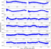 |
Fig. A.1 TESS photometric lightcurves of the Sector 9, 36, 62, 63, 89 and 90 |
This presents a set of robustness tests designed to evaluate whether the detected departure from strictly steady timing variations depends on the inclusion of specific sub-datasets, particularly the lower precision but temporally extensive TESS observations. Table A.3 compares the statistical performance of linear, quadratic, and cubic ephemeris models for datasets constructed with and without TESS timings.
TESS, with its space-based precision, provides extensive temporal coverage that is invaluable for long-term orbital analysis. However, its smaller aperture compared to ground-based telescopes like the Danish 1.54-m results in higher scatter in photometric measurements. The motivation for this comparative experiment is therefore not to reassess the dataset itself, but to determine whether the preference for the cubic ephemeris persists when the noisier TESS subset and outliers are removed.
Key observations and results: From the combined analysis from Table A.3 and A.4, the following conclusions include:
Across all data-quality cuts (full sample, best 20-40% timing precision, and removal of high-uncertainty or large-residual points), the cubic ephemeris consistently yields the lowest AIC and BIC values. This indicates that the increased model complexity is statistically supported rather than an artifact of any specific subset.
The inclusion of TESS data increases the overall χ2 and RMS residuals as expected from its higher photometric scatter but importantly, it does not erase or reverse the statistical preference for the cubic model. Both AIC and BIC continue to favor the cubic form in the “With TESS” and “Without TESS” cases.
For the highest-precision subsets (best 20-40 %), the cubic model maintains substantially lower information-criterion values, demonstrating that the non-linear curvature in the timing residuals is present even when the lowest-precision timestamps are removed.
To further test whether the cubic trend could be artificially driven by a few influential points, we also conducted a large-scale random hold-out cross-validation (Xval). In this test, 20 % of the transit times were randomly removed and the remaining 80 % refitted, repeated over 105 independent iterations. For each iteration, we compared the prediction errors of the linear, quadratic, and cubic ephemerides on the heldout data. Across all iterations, the cubic model produced prediction errors with a median absolute deviation comparable to the simpler models, while exhibiting the least systematic bias, indicating that the global curvature persists regardless of which measurements are withheld.
Statistical parameters for different subsets of the transit timing dataset.
In summary, this comparative analysis demonstrates that the detected departure from strictly steady timing variations is recovered regardless of whether TESS data are included. Although the TESS timings introduce additional scatter, both the AIC and BIC consistently favor the cubic ephemeris over the linear and quadratic forms, indicating that the increased model complexity is statistically warranted rather than an artifact of the lower-precision subset. Cross-validation experiments further confirm that the inferred curvature is not driven by isolated outliers or by any single sub-dataset. These results highlight the robustness of the non-linear trend detected in the timing residuals and underline the importance of continued, high-precision ground-and space-based monitoring to refine the long-term dynamical interpretation of the WASP-19 system.
Appendix B TTV analysis
This focused TTV analysis aims to test the possibility that the transit timing residuals observed in Fig. 3 are due to dynamical interactions with an unseen perturber in the WASP-19 system. To measure TTVs for TESS mid-transit times, we used opensource software allesfitter (Günther & Daylan 2019, 2021) that models the time-series TESS photometry data by performing MCMC built from the emcee (Foreman-Mackey et al. 2013) ensemble sampler and the corner (Foreman-Mackey 2016) package. We set the priors to run 100 000 steps with 200 walkers and 6000 burn-in steps to ensure a reasonable sampling process. After exploring all correlations in the parameter space, the TTVs and other orbital parameters can be accurately measured with their uncertainties estimated by the allesfitter software.
Mid-transit timing and photometric parameters for WASP-19 b used in this work.
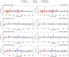 |
Fig. A.2 Transit timing residuals (O-C diagram) for WASP-19 b under different data inclusion scenarios. Each panel compares linear (solid black), quadratic (dashed green), and cubic (dotted brown) ephemeris models fitted to subsets of the data, with and without the inclusion of TESS transit timings. The top row shows results using all data, while the middle and bottom rows show fits restricted to the best 20%, 30%, and 40% of light curves based on photometric precision. Literature data are shown in red, Danish light curves (DK154) in blue, and TESS data in purple. |
Next, we applied the N-body simulation TTVFast (Deck et al. 2014) to evaluate the long-term TTV series. For a planetary system with a known transiting planet and a potential unseen perturber, this synthetic TTV series can be determined by first calculating the nth transit time and then subtracting the first two terms representing linear ephemerides (Hadden & Lithwick 2016, 2017):
![Mathematical equation: \begin{aligned} t(n) = T_{0} + nP_{b} + \mu' \delta t^{(0)}(n) + \mu' \mathrm{Re}[Z]\delta t^{(1,\,x)}(n) \\ + \mu' \mathrm{Im}[Z]\delta t^{(1,\,y)}(n), \end{aligned}](/articles/aa/full_html/2026/04/aa56822-25/aa56822-25-eq194.png) (B.1)
(B.1)
where μ′ represents the perturber’s planet-star mass ratio, and t(0)(n), t(1,x)(n), and t(1,y)(n) depend on the orbital period Pb and the reference time (or transit epoch) T0 of the inner planet. The variable Z:
 (B.2)
(B.2)
contains the free complex eccentricities of the inner planet  and the outer planet
  (Hadden & Lithwick 2016, 2017), ω and ω′ are their corresponding argument of periastron.
To derive the outer planet’s TTV series, we simply need to switch the following quantities:  ,
,  , and
, and  .
.
By fitting the measured TTVs with the synthetic TTV series, we can perform a separate MCMC to constrain the planetary mass (Mp) while exploring the parameter space of all input orbital parameters for TTVFast, including orbital period (Pb), eccentricity (e), inclination (i), longitude of the ascending node (Ω), argument of periastron (ω), and mean anomaly (M). The constrained planetary mass is  , which is consistent with the result reported in Table 2.
Statistical comparison of linear, quadratic, and cubic ephemeris models for WASP-19 b under different data-quality selections.
Statistical results of ephemeris model fits under different data-quality filtering criteria.
Furthermore, we extracted periodicity information from long-term synthetic TTV series using the Lomb-Scargle (LS) periodogram, a unique technique to detect and characterize periodic signals from unequally spaced data (Lomb 1976; Scargle 1982; VanderPlas 2018). In this paper, we applied this technique to explore the periodicity from the TTVFast model in Fig. 4 based on N-body simulations of gravitational interactions in planetary systems, not the cubic model in Fig. 3 that describes slow, non-periodic curvature expected from apsidal precession or tidal dissipation effects. Similar methodology can be found in other papers, such as Holczer et al. (2016) and Yahalomi & Kipping (2026). The LS periodogram for WASP-19b when searching for periodic signals up to 105 d is illustrated in Fig. B.1, where WASP-19b’s orbital period and its sub-harmonics (in the form of PWASP-19b/n, n = {2, 3,4,5,6,7,8,9,10}) are reflected as peaks in the upper panel. After removing all sub-harmonics in the middle panel of Fig. B.1, we found a power “excess” region at P ≳ 1200 d without long-period peaks being detected. The false alarm probability (FAP) returns to zero in this region, indicating that the LS signal is statistically strong and confident. Although the middle panel of Fig. B.1 shows a broad “excess” of power at periods P ≳ 1200 d once the sub-harmonics of the planetary orbital period are removed, this excess does not manifest as a distinct long-period peak. To assess whether this feature could still correspond to a genuine periodic modulation, we computed both analytic and bootstrap false-alarm probabilities (FAPs) using the measured TTV residuals.
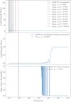 |
Fig. B.1 LS periodogram for WASP-19 b. The black dashed lines in the upper panel represent sub-harmonics of WASP-19 b’s periodic signal at P ≈ 0.789 d labelled with red dashed lines, while all sub-harmonics are removed in the middle panel. As a contrast, the corresponding FAP periodogram is illustrated in the lower panel. A long-period power "excess" region at P ≳ 1200 d is observed in the LS periodogram, but no obvious distant peaks are detected. |
The analytic FAP was evaluated using the classical expression for the exponential tail of the Lomb-Scargle periodogram under the null hypothesis of Gaussian noise (Lomb 1976; Scargle 1982; VanderPlas 2018):
![Mathematical equation: \mathrm{FAP_{analytic}} = 1 - \left[1 - e^{-z}\right]^{N_{\rm eff}},](/articles/aa/full_html/2026/04/aa56822-25/aa56822-25-eq214.png)
where z is the normalized LS power and Neff the number of independent frequencies. Applying this to the global peak power (z = 0.118) yields ~eq 0.95, indicating that the observed long-period excess is fully consistent with noise fluctuations.
To account for irregular sampling, we also performed a non-parametric bootstrap test FAPbootstrap by randomly shuffling the TTV residuals while keeping observation epochs fixed. For each of 104 realizations, a Lomb-Scargle periodogram was recomputed, and the highest peak was recorded. The resulting empirical false-alarm probability yields ∼eq 0.981 showing that nearly all bootstrap realizations produce peaks equal to or greater than the observed excess.
Together, the analytic and bootstrap tests demonstrate that the long-period power excess arises from baseline-limited spectral leakage rather than a coherent dynamical signal. This confirms that the LS periodogram does not contain statistically significant evidence of a long-period TTV modulation, and therefore does not support the presence of an additional planetary perturber in the WASP-19 system.
Appendix C Baseline correction for transmission photometric spectrum
To construct a consistent transmission spectrum from heterogeneous datasets, we applied a constant additive offset in transit depth to each instrument’s measurements. We adopted the HST STIS+WFC3 spectrum (Huitson et al. 2013) as the reference baseline due to its high signal-to-noise ratio, stable systematics, and continuous optical-near-IR coverage. For each ground-based or single-band dataset, we interpolated the HST spectrum onto the wavelength grid of that dataset within the overlapping region and solved for a constant offset ∆d that minimized the weighted squared difference between the datasets. Uncertainties in ∆d were estimated via bootstrap resampling. The resulting offsets are physically small (typically |∆d| ≲ 1.2 × 10⁻³), consistent with expected variations from unocculted stellar spots and instrumental baseline differences: for example, Huitson et al. (2013) report that unocculted spots can shift Rp/R* by up to 1.38% between epochs, corresponding to ∆d ~ (0.4-8) × 10−4, while Sedaghati et al. (2015) estimate a baseline uncertainty of −0.0017 in Rp/R* from FORS2 systematics. Similar vertical offsets are commonly applied in multi-instrument analyses (e.g., Bean et al. 2013; Mancini et al. 2013). Although we explored a broad prior range of ∆d ∈ [−0.02, +0.02] in transit depth, the best-fit values are more than an order of magnitude smaller, and for subsequent retrievals a tighter prior (e.g., ∆d ∈ [−5 × 10⁻³, +5 × 10⁻³] or a Gaussian prior with σ ≃ 0.001) is physically motivated. The final offsets applied in this work are shown in Table C.1. This homogenization ensures that the combined spectrum preserves the true wavelength-dependent atmospheric signal without being biased by instrument-specific baselines.
Offset corrections applied to each WASP-19b dataset.
Derived photometric parameters from each light curve, plus the interval within which the best fit was searched for using GEMC.
All Tables
Statistical comparison of linear, quadratic, and cubic ephemeris models for WASP-19 b under different data-quality selections.
Statistical results of ephemeris model fits under different data-quality filtering criteria.
Derived photometric parameters from each light curve, plus the interval within which the best fit was searched for using GEMC.
All Figures
|
Fig. 1 Observations of 27 transits were conducted from 2015 to 2023 utilizing the DFOSC instrument on the Danish Telescope at La Silla Observatory. Transits that exhibit possible starspots are enclosed within rectangular markers. The observation dates follow the YY/MM/DD format. |
| In the text | |
|
Fig. 2 Light curves of transits observed with the Danish telescope, with starspots modeled using PRISM+GEMC, along with the corresponding residuals. |
| In the text | |
|
Fig. 3 Transit-timing residuals of WASP-19 b with respect to the best-fitting linear ephemeris. The red, blue, and purple points represent literature, Danish, and TESS data, respectively, with their associated timing uncertainties. The solid black, green, and brown curves correspond to the median fits from the linear, quadratic, and cubic polynomial models, respectively. Shaded regions indicate the 68 % confidence intervals derived from 20000 bootstrap realizations of each model’s MCMC posterior distribution. |
| In the text | |
|
Fig. 4 Measured TTVs derived from allesfitter when modeling TESS observations for WASP-19 b in the upper plot with their residuals illustrated in the lower plot. The TTVFast model yields a negligible TTV amplitude of ATTV = 1.102 × 10⁻⁶ min. |
| In the text | |
|
Fig. 5 MEGNO stability map depicting the upper mass limit (within ±1σ (68.3%), ±2σ (95.4%), and ±3σ (99.7%) confidence intervals) of an injected hypothetical perturber in the WASP-19 system. The red horizontal dashed lines represent the perturber’s mass range between M = 400 M⊕ and M = 1.4 M⊕ determined from the RV constraints (Bernabò et al. 2024). The red vertical dashed lines from left to right represent the perturber’s unstable orbits in 2:3, 1:1, and 3:2 resonances with WASP-19b determined in this paper, while the black vertical dashed lines from left to right represent the perturber’s stable orbits in 1:2, 5:3, 2:1, 5:2, and 3:1 resonances with WASP-19b found by Cortés-Zuleta et al. (2020). |
| In the text | |
|
Fig. 6 Variation of the planetary radius, expressed as transit depth, as a function of wavelength. Sky-blue points correspond to Danish-DFOSC (this work), lime to TESS (this work), orange to GROND (Mancini et al. 2013), crimson to MMIRS (Bean et al. 2013), green to Sedaghati et al. (2015), and black to Huitson et al. (2013). Vertical error bars represent measurement uncertainties, while horizontal bars indicate the full width half maximum (FWHM) of the respective passbands. Synthetic photometric points were computed using the SVO SpecPhot tool to obtain flux-weighted transit depths at the effective wavelengths of the UV-optical filters. Retrievals were performed with POSEIDON including the opacities of Na, K, TiO, VO, and H2O. The orange curve shows the median best-fit model excluding TiO and VO, with 1σ and 2σ confidence intervals. The purple curve shows the median best-fit model including TiO and VO, with corresponding uncertainties. See Sect. 6.2 for details. |
| In the text | |
|
Fig. A.1 TESS photometric lightcurves of the Sector 9, 36, 62, 63, 89 and 90 |
| In the text | |
|
Fig. A.2 Transit timing residuals (O-C diagram) for WASP-19 b under different data inclusion scenarios. Each panel compares linear (solid black), quadratic (dashed green), and cubic (dotted brown) ephemeris models fitted to subsets of the data, with and without the inclusion of TESS transit timings. The top row shows results using all data, while the middle and bottom rows show fits restricted to the best 20%, 30%, and 40% of light curves based on photometric precision. Literature data are shown in red, Danish light curves (DK154) in blue, and TESS data in purple. |
| In the text | |
|
Fig. B.1 LS periodogram for WASP-19 b. The black dashed lines in the upper panel represent sub-harmonics of WASP-19 b’s periodic signal at P ≈ 0.789 d labelled with red dashed lines, while all sub-harmonics are removed in the middle panel. As a contrast, the corresponding FAP periodogram is illustrated in the lower panel. A long-period power "excess" region at P ≳ 1200 d is observed in the LS periodogram, but no obvious distant peaks are detected. |
| In the text | |
Current usage metrics show cumulative count of Article Views (full-text article views including HTML views, PDF and ePub downloads, according to the available data) and Abstracts Views on Vision4Press platform.
Data correspond to usage on the plateform after 2015. The current usage metrics is available 48-96 hours after online publication and is updated daily on week days.
Initial download of the metrics may take a while.