| Issue |
A&A
Volume 708, April 2026
|
|
|---|---|---|
| Article Number | A366 | |
| Number of page(s) | 16 | |
| Section | Astrophysical processes | |
| DOI | https://doi.org/10.1051/0004-6361/202556613 | |
| Published online | 27 April 2026 | |
The MARTINI platform
I. Se I–X atomic calculation and expansion opacity for early stage kilonova spectral analysis
1
Department of Physics, Sapienza University of Rome, P.le A. Moro 5, 00185 Rome, Italy
2
National Institute for Astrophysics – Astronomical Observatory of Abruzzo, Via Maggini snc, 64100 Teramo, Italy
3
National Institute for Nuclear Physics – Section of Perugia, Via A. Pascoli, Perugia, Italy
4
Department of Physics and Earth Science, University of Ferrara, Via Saragat 1, I-44122 Ferrara, Italy
5
National Institute for Nuclear Physics – Section of Ferrara, Via Saragat 1, I-44122 Ferrara, Italy
6
Institute of Theoretical Physics and Astronomy, Vilnius University, Saulėtekio Ave. 3 Vilnius, Lithuania
★ Corresponding author: This email address is being protected from spambots. You need JavaScript enabled to view it.
Received:
26
July
2025
Accepted:
22
February
2026
Abstract
Context. In the multi-messenger era, kilonovae represent key sites of r-process nucleosynthesis, making opacity estimation and spectral analysis crucial for constraining their composition.
Aims. Since light r-process elements shape the early (∼0.5 − 1.5 d) ejecta opacity, we present a detailed study of selenium with a focus on atomic data calculation, expansion opacity estimation, and spectral analysis.
Methods. We calculated the selenium atomic data from Se I to Se X using the GRASP2018 code. We performed a systematic analysis and evaluation of their precision through a detailed comparison with the NIST ASD, and other works available in the literature. We then used these atomic data to estimate expansion opacity at different temperatures (e.g. T = 5000 K, 10 000 K, 20 000 K, 100 000 K) and densities (e.g. ρ = 10−13 g cm−3, 3 × 10⁻¹² g cm−3). We performed spectral analysis with the Monte Carlo radiative transfer code POSSIS, with a pre-computed opacity grid calculated with new densities and temperatures, ranging from −19.5 to −4.5 g cm−3 in log-scale and from 1000 to 51 000 K, respectively. In the analysis, we considered two scenarios: one in which the opacity contribution comes from 100% selenium ejecta, and another in which selenium only partially contributes to the total opacity (∼10% of the total mass).
Results. The selenium atomic calculations show a good agreement with NIST ASD, with accurate energy levels and transitions determined alongside atomic data for higher ionisation stages not fully covered by NIST ASD. The expansion opacities calculated with these new selenium data exhibit differences in comparison to existing works in the literature. Selenium spectral features can only be observed in the kilonova scenario consisting of 100% selenium. When selenium accounts for about 10% of the total kilonova mass, these features become undetectable. Finally, all selenium results are now available in the new open-source MARTINI platform dedicated to element nucleosynthesis.
Key words: gravitational waves / atomic data / opacity / radiative transfer
© The Authors 2026
 Open Access article, published by EDP Sciences, under the terms of the Creative Commons Attribution License (https://creativecommons.org/licenses/by/4.0), which permits unrestricted use, distribution, and reproduction in any medium, provided the original work is properly cited.
This article is published in open access under the Subscribe to Open model. This email address is being protected from spambots. You need JavaScript enabled to view it. to support open access publication.
1. Introduction
Modern astronomy is characterised by an ever-growing stream of observational data. The international astrophysics community has been, and continues to be, inundated with spectroscopic data from numerous large-scale surveys (e.g. Gaia-ESO (European Southern Observatory): Randich et al. 2022; GALAH (GALactic Archaeology with HERMES, High Efficiency and Resolution Multi-Element Spectrograph): De Silva et al. 2015; APOGEE (Apache Point Observatory Galactic Evolution Experiment): Majewski et al. 2017; 4MOST (4-metre Multi-Object Spectroscopic Telescope): Guiglion et al. 2019; WEAVE (WHT Enhanced Area Velocity Explorer): Jin et al. 2024). Handling such a vast volume of data requires substantial theoretical efforts to accurately reconstruct the evolution of chemical abundances across time and space for the different components of our Galaxy, as well as in nearby galaxies.
Stellar yields are key ingredients in chemical evolution models. Some of them relate to stars that do not ignite carbon in their cores and end their evolution as white dwarfs, after passing through the asymptotic giant branch (AGB) phase (see, e.g. Busso et al. 1999; Straniero et al. 2006). These stars are responsible for producing roughly half of the elemental abundances heavier than iron via the slow neutron-capture process (s-process; Gallino et al. 1998).
The remaining half are produced by massive stars: via the weak s-process (e.g. Pignatari et al. 2010) during their pre-explosive phases, and – whether as single stars or members of binary systems – via the rapid neutron-capture process (r-process; see, e.g. Cowan et al. 2021) during their final evolutionary stages. While the r-process yields of individual sites can vary due to the uncertainties in modelling the late evolutionary phases of stars, this does not substantially affect the global r-process abundance pattern. S-process nucleosynthesis is anchored in laboratory measurements of all relevant reaction rates and half-lives, whereas the r-process relies largely on theoretical extrapolations for nuclei that are far from stable. For this reason, it is generally more robust to derive the solar r-process fraction as r = 1 − s (see e.g. Prantzos et al. 2020), rather than inferring the s-process contribution from 1 − r.
Interest in the r-process has surged in recent years following the gravitational wave event GW170817 (Abbott et al. 2017a), which was triggered by the coalescence of a binary neutron star (BNS) system. The GW170817 event was groundbreaking, as it marked the advent of multi-messenger astronomy (Abbott et al. 2017a; Corsi et al. 2024). The gravitational wave (GW) detection was accompanied by electromagnetic counterparts. In particular, GW170817 included a short gamma-ray burst, identified as GRB170817A (Abbott et al. 2017b; He et al. 2018; Lyman et al. 2018) and a kilonova (KN) emission stemming from the radioactive decay of r-process elements synthesised during the merger (AT2017gfo; Andreoni et al. 2017; Arcavi et al. 2017; Cowperthwaite et al. 2017; Drout et al. 2017; Evans et al. 2017; Kasliwal et al. 2017; McCully et al. 2017; Pian et al. 2017; Smartt et al. 2017; Soares-Santos et al. 2017; Utsumi et al. 2017). The KN provided the first direct evidence of in situ production of heavy elements via the r-process (e.g. Pian et al. 2017). However, theoretical modelling of KNe requires a complex set of physical inputs, ranging from nucleosynthesis yields and thermalisation coefficients to line opacities of the individual chemical elements produced (e.g. Kasen et al. 2015; Metzger 2019).
Most recent studies, such as Banerjee et al. (2022, 2024), Fontes et al. (2023), Flörs et al. (2023), Carvajal Gallego et al. (2024), and Kato et al. (2024), have focused on lanthanides and actinides, which undoubtedly play a significant role in KN opacity. However, much less attention has been paid to non-lanthanide elements present in early stage (∼0.5–1.5 days after the merger) evolution, especially at high-ionisation states. During this phase, light elements play a key role in shaping the early spectrum (Kasen et al. 2013; Villar et al. 2017; Metzger 2019). Figure 1 shows typical abundances of light r-process elements synthesised in the high-Ye (high electron fraction) dynamical polar ejecta and spiral-wave ejecta of BNS mergers.
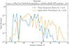 |
Fig. 1. Abundances of light r-process elements for trajectories representative of the dynamical polar wind and spiral-wave wind, at 1.5 days after merger. For both trajectories, selenium accounts for about 10% of the total mass. |
These lanthanide-poor components, which are the earliest and fastest ejecta, can dominate the blue kilonova emission during the first days after the merger (Nedora et al. 2019; Perego et al. 2022). The dynamical polar (Ye = 0.35) trajectories and spiral-wave (Ye = 0.30) trajectories shown here are representative examples of their respective ejecta types (Vescovi et al. 2022). In the dynamical polar case, nucleosynthesis produces Sr as the heaviest abundantly produced element, while the spiral-wave trajectory may also produce interesting elements such as Y, Mo, and Pd. There are studies available in the literature that investigated strontium (Watson et al. 2019; Perego et al. 2022; Domoto et al. 2022; Sneppen et al. 2024), while less attention has been paid to other elements, such as yttrium (Sneppen & Watson 2023), zirconium (Domoto et al. 2022), palladium, molybdenum, and selenium (Se), which are abundantly produced through the r-process. Moreover, their relatively simple atomic structure makes them easier to handle in both theoretical and experimental studies, providing valuable information on the opacity under KN conditions (Mascali et al. 2022; Pidatella et al. 2021; Bezmalinovich et al. 2024).
To reduce the lack of data for highly ionised states of non-lanthanide elements, in this first article, we present a study focused on selenium (Se) I–X atomic data and expansion opacity calculation in the framework of early stage KN. While our long-term goal is to include all elements and perform fully consistent KN modelling, in this work we only investigate Se because it is one of the most abundant element produced by ejecta with high electron fractions (Ye = 0.3 − 0.35) and a mass fraction XSe = 0.1 (Fig. 1) in early stage scenario. Moreover, Se was chosen as it is among the primary candidates for future measurement at PANDORA (Plasmas for Astrophysics Nuclear Decays Observation and Radiation for Archaeometry; Mascali et al. 2022), a magnetic trap facility currently under construction at the INFN – Laboratori Nazionali del Sud in Italy. Therefore, investigating its atomic properties and opacity is essential in view of future experiments and KN modelling.
Prompted by the need for these data from both theoretical and experimental communities, we created a new online platform, MARTINI1, which is designed to provide researchers with the inputs needed to simulate the chemical evolution of the Galaxy and to model KN light curves.
The paper is divided into the following sections. In Sect. 2, we begin with a theoretical introduction to KN and expansion opacity. Moreover, we provide a brief presentation of the GRASP2018 (general relativistic atomic structure package) atomic code developed by Froese Fischer et al. (2019), employed for the atomic calculation, and the KN code POSSIS (POlarization Spectral Synthesis In Supernovae; Bulla 2019, 2023). Sect. 3 is entirely dedicated to Se atomic calculations and to the computational strategy adopted. Specifically, starting from the available works of Tanaka et al. (2020), Radžiūtė & Gaigalas (2022), and Kitovienė et al. (2024), we performed Se atomic calculations, with the aim of improving the accuracy of Se I–IV energy levels and transitions compared to the NIST ASD2 (National Institute of Standards and Technology atomic spectra database; Kramida & Ralchenko 1999). We extended our approach to higher ionisation states, from Se V to Se X. These atomic results were then used to estimate the expansion opacity, the results of which are reported in Sect. 4. Finally, in Sect. 5 we incorporate the opacity results into POSSIS to analyse and investigate KN spectral features.
2. Theoretical background
2.1. Kilonova physics
Kilonovae occur during the post-merger phase of a BNS or black hole – neutron star (BHNS) system shortly after mass ejection (Radice et al. 2020). They are quasi-thermal electromagnetic transients powered by the radioactive decay of heavy neutron-rich isotopes synthesised in the aftermath of BNS or BHNS mergers (Kasen et al. 2017; Metzger 2019). The peak luminosity and colour of the transient depend on several factors (e.g. ejecta mass, velocity, composition) and can evolve with time. For AT2017gfo, the KN initially peaked in the near-ultraviolet and optical range, pushing to infrared emissions as soon as the ejected material expanded and cooled (e.g. Chornock et al. 2017)
The study of KNe offers a unique opportunity to investigate the conditions under which heavy elements are synthesised and their subsequent distribution in the cosmos. The extreme neutron-rich environment of KN ejecta allows the efficient synthesis of heavy elements, such as gold, platinum (Gillanders et al. 2021), and the majority of elements beyond the second r-process peak (A ≥ 130).
However, due to several factors that are not yet well understood (e.g. the EoS (equation of state), the mass ratios of neutron stars, nuclear physics rates and half lives, the role of neutrinos, mass ejection processes, timescales), it is challenging to precisely determine the exact composition of the ejecta emitted from a BNS. One approach to addressing this issue involves analysing the observed spectra of the KN. Consequently, it is necessary to overcome uncertainties in opacity calculations, which often arise from oversimplified atomic structure models (Barnes et al. 2016; Kasen & Barnes 2019; Tanaka et al. 2020), to ensure precise spectral analysis and resolve between theoretical predictions and observational data for KNe.
2.2. The expansion opacity
Kilonova opacity is dominated by bound-bound transitions. Following previous studies (Kasen et al. 2013; Barnes & Kasen 2013; Tanaka & Hotokezaka 2013; Tanaka et al. 2020), we computed the expansion opacity using the formalism for bound-bound lines (Sobolev 1960; Castor 1974; Karp et al. 1977), combined with the formula by Eastman & Pinto (1993). During the post-merger phase of a BNS system, the ejecta expand at high velocities, vej, following the laws of homologous expansion with a timescale, t (this assumption may break down in the case of circumstellar material plasma through which the ejecta propagate). In this scenario, the spectral lines generated are broadened because of the dynamics of the ejecta.
The expression for calculating the opacity within a bin in an expanding medium is defined by the so-called bound–bound expansion opacity (Eastman & Pinto 1993; Banerjee et al. 2020):
 (1)
(1)
where texp refers to the time elapsed since the material was ejected, ρ is the density, c the speed of light, and λl is the wavelength of the corresponding l transition within the bin, Δλ. The Sobolev optical depth, τl, is defined as
 (2)
(2)
with fl being the oscillator strength, nℓ the density population of ℓ-level, and me and e the mass and charge of the electron, respectively.
In the literature, there are two other approaches that are frequently used to calculate opacity. One is the line-binning method (e.g. Fontes et al. 2020), while the other is the line-by-line method (e.g. Shingles et al. 2023). The former consists of grouping spectral lines into wavelength bins and calculating the opacity within each bin, without including the ‘expansion’ of the medium (typically for the expansion opacity). In the latter technique, the opacity is calculated for each individual line with no bin considerations.
Calculating the expansion opacity requires detailed atomic data inputs. Following previous works (Tanaka et al. 2020; Banerjee et al. 2022, 2024; Pognan et al. 2022), we assumed local thermodynamic equilibrium (LTE), which is a reasonable approximation in the early phase of KNe (< 2–3 days). Through the Saha equation, we determined the ionisation balance. This equation relates two adjacent stages of ionisation, i and i + 1, and is defined as:
 (3)
(3)
where kB is the Boltzmann constant, ne is the electron number density, h is the Planck constant, χi is the ionisation potential of the ith ionisation degree, and Ui(T) is the partition function for the ith ionisation state defined as:
 (4)
(4)
where gi, ℓ is the statistical weight corresponding to the energy, Ei, ℓ, of the level, ℓ. Once the ionisation balance is determined, the Boltzmann distribution specifies the relative population of excited levels within a given ionisation stage,
 (5)
(5)
where ni, ℓ is the density population of ℓ-level with respect to the total population ni of the ith ionisation stage.
As shown in Eq. (1), atomic calculations are essential to accurately compute the expansion opacity. In this context, we used the GRASP2018 atomic code.
2.3. The theory behind GRASP2018
GRASP2018 is a general relativistic atomic structure package developed by Froese Fischer et al. (2019) based on fully relativistic (four-component) multi-configuration Dirac-Hartree-Fock (MCDHF) and relativistic configuration interaction (RCI) methods (Grant 2007; Fischer et al. 2016), suitable for medium to heavy atomic systems. Starting from the eigenvalue equation  ,
,  is the Dirac-Coulomb Hamiltonian, defined as
 (6)
(6)
with V the interaction potential between N total electrons, rjk the distance of electron–electron repulsion between two distinguished electrons (j, k), α and β the Dirac matrices, and p the momentum operator. The MCDHF method is applied to  to determine a numerical representation of the atomic state function (ASF) ψ as
 (7)
(7)
obtained by the linear combination of configuration state functions (CSF) Φ(γrPJMJ), eigenfunctions of the parity P, total angular momentum operators J2, and its projection MJ, with the mixing coefficients cr (Kitovienė et al. 2024).
GRASP2018 performs a single run per element per ionisation state. It starts with a set of electron configurations (ECs) provided as input to determine a multi-reference (MR) set, followed by the estimation of the radial part of the wave function. In addition, angular integrations based on the second quantisation formalism (Gaigalas et al. 2001a, 2017) are included, together with Breit interaction and quantum electrodynamic (QED) corrections applied to the RCI computation. Finally, the energy levels and transitions are determined.
2.4. KN spectra modelling: POSSIS
Once the atomic calculations are performed, it is possible to estimate the expansion opacity, and the results are then inserted as input into POSSIS (Bulla 2019, 2023), which is a three-dimensional Monte Carlo radiative transfer code that can model radiation transport in expanding media like the ejecta of supernovae and KNe. Unlike other sophisticated radiative transfer codes available in the literature (e.g. Höeflich et al. 2021; Blinnikov et al. 1998; Hauschildt & Baron 1999; Utrobin 2004; Dessart & Hillier 2005; Kasen et al. 2006; Kromer & Sim 2009; Tanaka & Hotokezaka 2013; Wollaeger & van Rossum 2014; Kerzendorf & Sim 2014), POSSIS uses pre-computed atomic opacity tables as the input, which can significantly speed up the calculation time. The code includes wavelength- and time-dependent opacities and generates angular-dependent predictions of spectra, light curves, and polarisation for both simplified and hydrodynamical explosion models. We report below the key aspects of the code’s structure and focus particularly on the latest version of the code (Bulla 2023) that is used in this work. More details can be found and studied accurately in Bulla (2019) and Bulla (2023).
First, the ejecta are described by a 3D Cartesian grid specifying the ith spatial coordinates, density, ρi, 0, and electron fraction, Ye, i, at a reference time, t0, for each cell. The time-dependence is modelled assuming homologous expansion, i.e. the velocity and mass of each cell is constant and therefore radial coordinates and densities scale with time, t, as ri ∝ t and ρi ∝ t−3, respectively. We assume Ye, i to remain constant within each cell, i.e. the composition is fixed during the simulation.
Key properties that control the energy budget and set the temperature profile of the ejecta are the nuclear heating rates,  , and the thermalisation efficiencies, ϵth. We took the nuclear heating rates, which provide the amount of energy per unit time per unit mass produced by the radioactive decay of r-process nuclei, from Rosswog & Korobkin (2024). In this framework, the electron fraction, Ye, and the expansion velocity, vexp, only enter as input parameters required to select the appropriate heating rate prescription and are therefore fixed to their initial values within each cell. Although Ye and the chemical composition may evolve with time, this evolution is not explicitly followed, as its effect is already captured by the time dependence of the tabulated heating rates. Instead, the expansion velocity is computed at the start of the simulation as a function of the cell mass and the cell width in velocity space, which remain constant under homologous expansion. As a result, for each cell the heating rate depends solely on time. The thermalisation efficiencies, which control what fraction of the heating rates thermalise within the ejecta and is available to power the KN, are computed within the code following standard prescriptions (Barnes et al. 2016; Wollaeger et al. 2018).
Assuming perfect coupling between matter and radiation, heating rates and thermalisation efficiencies are then used to initialise the temperature of the ejecta. Specifically, the mean intensity of the radiation field in each cell is computed as
 (8)
(8)
and the ejecta temperature is set equal to the radiation temperature, Ti, estimated via the Stefan-Boltzmann law:
 (9)
(9)
In the two equations, the texp/ts term accounts for adiabatic energy losses from a given time, texp < ts, to the starting time of the simulation, ts, and σ is the Stefan-Boltzmann constant. During the simulation, the temperature is updated at the end of every time step using Monte Carlo estimators (Mazzali & Lucy 1993; Lucy 2003) in Eq. (9) for the mean intensity,
 (10)
(10)
where V is the cell volume and the sum is performed over all the Monte Carlo photon packets with co-moving-frame energy, ecmf, travelling a path length, Δl, through the given cell at the given time step with duration, Δt.
Once the grid structure is set, a number, Nph, of identical and indivisible Monte Carlo photon packets (Abbott & Lucy 1985) are created and spread evenly across the different time steps. Monte Carlo photons activated at a given time step are assigned initial positions, x, initial directions, n, energies, e, frequencies, ν and normalised Stokes vectors, s. The initial energy of all packets is the same (Abbott & Lucy 1985) and computed by evenly splitting the energy from the radioactive decay of r-process nuclei thermalised within the ejecta (Wollaeger et al. 2018; Rosswog & Korobkin 2024). The initial frequency, ν, is chosen by sampling the thermal emissivity
 (11)
(11)
where κtot(ν) is the total opacity and B(ν, T) is the Planck function at temperature T.
The propagation of Monte Carlo packets is then controlled by the opacities of the expanding medium. In particular, the code POSSIS takes as input tables specifying electron-scattering and bound-bound opacities as a function of wavelength, time and local ejecta properties like density, temperature and electron fraction3. The output flux and polarisation spectra as a function of time are then constructed ‘on the fly’ using estimators (Kerzendorf & Sim 2014; Bulla et al. 2015), a technique that leads to a significant reduction in numerical noise compared to the binning of escaping packets commonly used in Monte Carlo radiative transfer simulations.
3. Atomic calculation
3.1. GRASP2018 calculation strategy
We started by focusing on the first four degrees, I–IV, of Se (i.e. Se I, Se II, Se III, and Se IV). A MR set of ECs must be defined to determine the CSFs for the ASF, as seen in Eq (7). Table 1 reports the MR sets of the ECs selected for the calculation of Se I–IV.
Se I–IV electron configurations.
The ECs were divided by parity, and their relative wave functions were optimised separately according to even or odd states. The choice of ECs was guided by references such as the NIST ASD (Kramida & Ralchenko 1999) and articles available in the literature by Tanaka et al. (2020), Radžiūtė & Gaigalas (2022), and Kitovienė et al. (2024). Moreover, we performed our calculations by respecting the same orbital symmetry between even and odd states for all the degrees of ionisation, ensuring convergence within GRASP2018. At odds with the work of Tanaka et al. (2020), our calculation included f shell orbitals for Se I–IV. On the one hand, this approach allows us to highlight possible differences between the two works; on the other hand, it enables a well-founded comparison with NIST ASD and the two works Radžiūtė & Gaigalas (2022) and Kitovienė et al. (2024), both of which provide f shell ECs. To calculate the energy levels and the transitions, we included single-double (SD) excitation applied to the valence shell, while keeping the core [Ar]3d10 and the 4s2 shells frozen during the whole calculation. For each ionisation stage, we applied the same computational strategy. Once Se I–IV were completed, the procedure was extended to Se V–X, using the corresponding ECs reported in Table 2.
Se V–X electron configurations.
In particular, Se V was computed by adopting the same calculation strategy as in the lower ionisation stages. Starting from Se VI, a slight modification to this approach became necessary. Specifically, in the cases of Se VI and VII, the orbital symmetry involving the subshells {5s, 5p, 4d, 4f} was not preserved between the even and odd parity states, as this adjustment was required to ensure the convergence of the code. Beyond Se VII, the f shell was no longer included, because the valence electrons in these higher ionisation states primarily occupy the s, p, and d shells. Given the high temperature (≳10 000 K) of the medium, electrons are more likely to be ionised rather than excited to the f shell. Furthermore, from Se VIII, the [Ne] core was treated as frozen throughout the entire calculation, including a new orbital symmetry {5s, 5p, 4d} between even and odd states. Finally, the case of Se IX and X is complicated by the lack of guidance from the NIST ASD, which does not provide information on possible ECs. To address this gap, a set of ECs was independently defined, with a focus on improving the transition probabilities and improving the accuracy of the ASF, thus strengthening the final opacity calculations.
In GRASP2018, RCI correlations with MR sets are included, taking into account a set of virtual orbitals with a step-by-step procedure through different layers. In our calculation, we assumed three different layers, starting from the initial L1 to the final layer L3.
As shown in Table 3, the adopted layer structure varies across the Se I to Se X calculations. This is necessary to ensure convergence of the atomic calculations, and to optimise the final energy levels and atomic transitions. In this regard, to correctly estimate the accuracy of the calculated energy levels, we computed mean absolute differences between energy levels, following the methodology presented in Radžiūtė & Gaigalas (2022). In detail, this approach consists in computing the mean absolute differences and the mean relative differences between the predicted energy levels and those reported in the NIST ASD database, which serves as the reference. The equations used for these calculations are defined as
 (12)
(12)
 (13)
(13)
List of RCI layers.
where E* denotes the energy level under investigation, to be compared with the corresponding value of the NIST ASD database, in a total of N energy levels in common between the references (i.e. Tanaka et al. 2020; Radžiūtė & Gaigalas 2022; Kitovienė et al. 2024). Identification of the levels obtained in the GRASP package is usually performed in the jj-coupling scheme. Therefore, in order to compare the obtained levels with the NIST ASD database, where levels are usually identified in LS-coupling (coupling between the total angular momentum, L, and the total spin, S), it is necessary to perform a transformation of the atomic state function from jj-coupling to LS-coupling (Gaigalas et al. 2001b, 2003). This transformation is performed by the jj2lsj program (Gaigalas et al. 2004, 2017), which is integrated into the GRASP package (Froese Fischer et al. 2019). This identification of levels by LS-coupling and comparison with the NIST ASD database is approved by the atomic theory community.
To broaden the analysis and achieve a complete and consistent evaluation, in addition to our Se results, we include available atomic data from the literature. We consider atomic results for Se II and Se III performed with GRASP2018 and published by Radžiūtė & Gaigalas (2022) and Kitovienė et al. (2024), respectively, and Se I–IV data published by Tanaka et al. (2020) and available from the online database4 Japan–Lithuania (Kato & Tanaka 2021) calculated using the HULLAC atomic code (Bar-Shalom et al. 2001).
Finally, we adopted the same strategy and the quantitative and qualitative evaluation (QQE) method described in the work of Kitovienė et al. (2024) to evaluate the accuracy of the calculated transitions. The strategy consisted in evaluating the derived transitions in different classes, based on the ASF accuracy of the wave function introduced in Eq. (7). The classes are as follows: AA, A+, A, B+, B, C+, C, D+, D, and E. Class E indicates a transition with low ASF accuracy, while AA represents the class with the highest.
3.2. Se atomic calculation results
Since our goal is to calculate the expansion opacity arising from bound-bound transitions, we restricted our analysis to bound-state energy levels only. We first report the results inherent in the energy levels of Se I–IV and Se V-X. Secondly, the resulting atomic transitions of all ionisation stages are presented.
Fig. 2 shows a comparison of the energy levels predicted by this work, and the published data of Tanaka et al. (2020), Radžiūtė & Gaigalas (2022), and Kitovienė et al. (2024). The results of each work are compared with the NIST ASD and the error estimates are provided in Table 4.
 |
Fig. 2. Se I–IV energy levels of the four works compared with the NIST ASD. In the analysis we considered all energy levels below ionisation for each state. The dashed lines represent the ionisation threshold for each ionisation degree. |
Se I–IV error estimation of the energy levels.
Our Se I–IV calculations show good agreement with the NIST ASD and appear to be more accurate than the data reported in Tanaka et al. (2020) (see Fig. 2 and Table 4). These differences in precision and number of energy levels, compared to Tanaka et al. (2020), may be attributed to several factors, like the computational strategy (e.g. the inclusion of f shells in the ECs and RCI method adopted; see Tables 1 and 3) or the different atomic code used in the calculation. Specifically, the accuracy of our Se I and Se IV energy levels improves by approximately 3% and 5%, respectively, while Se II and Se III show improvements around 2% and 1%, respectively. In this respect, we stress that the uncertainty of the Se IV ionisation state is more than halved with respect to previous available publications. Furthermore, our findings for Se II and Se III demonstrate that the works of Radžiūtė & Gaigalas (2022) and Kitovienė et al. (2024) agree better with the NIST ASD, with results approximately two times more accurate than ours. Since the assumptions made by the two models are the same as those used by us (i.e. same atomic code and same inclusion of f shell in ECs), these differences in the results highlight the need for a dedicated refinement of the choice of ECs and the RCI layer method in our GRASP2018 calculations for each ionisation stage. However, achieving this level of precision in the results requires a huge effort and a very sophisticated computational procedure that takes months or even years to complete. In this context, our method sought a solution that is certainly less accurate but still provides a good level of precision of the data, allowing calculations to be feasible in a short time (from approximately a few weeks to a few months). Moreover, the goal of our work is to provide reliable atomic data for several atomic elements, starting from the Se calculations presented in this work. Although not precisely as accurate as in Radžiūtė & Gaigalas (2022) and Kitovienė et al. (2024), the computational strategy we adopted demonstrates that the obtained Se results are in good agreement with the NIST ASD reference, and better reproduce accurate energy levels of Se I–IV than existing works in the literature (e.g. Tanaka et al. 2020).
Further confirmation of the accuracy of the energy levels is obtained from the ionisation fraction plot. Fig. 3 reports the ionisation fraction of our Se I–IV as a function of the temperature. This plot is obtained by applying the Saha-Boltzmann equations (see Eqs. (3) and (5)) to the atomic levels presented in Table 4 to correctly estimate the ionisation states and the population distribution. In the same plot, we compare our Se I–IV results with the ionisation fraction calculated for another two models. ‘Model I’ is formed by the inclusion of Radžiūtė & Gaigalas (2022) Se II and Kitovienė et al. (2024) Se III with our Se I and Se IV to create a model with the highest accuracy of Se data compared to the NIST ASD. The other model considers the Se I–IV atomic data of Tanaka et al. (2020). First of all, we see that the level population of our Se I–IV overlaps with the other two models, which means that our Se I–IV energy levels that contribute to the partition function have been estimated correctly.
 |
Fig. 3. Se ionisation fraction as a function of the temperature. Vertical dashed lines indicate the temperature at which a new ionisation state is rising. The blue panel represents the range of temperatures of interest for the early stage KN (≳10 000 K). |
Moreover, from Fig. 3, it can be evinced that Se I and Se II do not impact as much as Se III and Se IV in the range of interest for early stage KNe. Rather, the ionisation fraction plot suggests that Se V should be taken into account for a more accurate modelling of KNe at these temperatures.
Beyond Se IV, only the theoretical models of Banerjee et al. (2024) are available in the literature, but without published or accessible data to be used for the analysis. Therefore, the evaluation of our results is only based on a comparison with the NIST ASD database. Fig. 4 presents the calculated energy levels from Se V to Se X, with their respective error estimates listed in Table 5.
 |
Fig. 4. Se V–X energy levels of our GRASP2018 atomic calculations compared with the NIST ASD. In the analysis we considered all energy levels below ionisation for each state. The dashed lines represent the ionisation threshold for each ionisation degree. |
Se V–X error estimation of the energy levels.
Table 5 shows that the accuracy of the Se V–VIII calculations is even higher than the Se I–IV ones. The precision of Se V and Se VII is within 2,5%, while Se VI and Se VIII show deviations of less than 2%.
As can be seen in Fig. 4, an exception has to be made for Se IX and X for which no NIST data are provided. In these two cases, the reliability of the results only depends on the quality of the level transitions calculated using the method described in Sect. 3.1. In Fig. 5, we report all transitions obtained from Se I to Se X with the corresponding classes. The classification proves that E-class transitions dominate at lower ionisation stages, while this trend reverses as we move towards higher stages. This indicates that the ASFs obtained for Se I–III are less accurate compared to those for Se IV–X. A similar conclusion can be reached by comparing our calculated transitions for Se II and Se III with the works of Radžiūtė & Gaigalas (2022) and Kitovienė et al. (2024), presented in Fig. 6.
 |
Fig. 5. Se I–X transition classes of GRASP2018 calculation. In the legend, ‘AA’ denotes transitions computed with highly accurate wave functions, whereas ‘E’ indicates the least accurate ones. |
 |
Fig. 6. Se II–III transition classes of our GRASP2018 atomic calculations compared with Radžiūtė & Gaigalas (2022) Se II, and Kitovienė et al. (2024) Se III. |
However, in the early stage scenario, the dominant ionisation stages are those beyond Se IV. Therefore, considering the high quality of these transitions (Fig. 5), together with the high accuracy achieved on the energy levels (Table 5), we provide a robust estimation for Se expansion opacity. Moreover, the Se I–X data presented and discussed in this section can be integrated into the MARTINI platform to support future KN modelling.
4. Expansion opacity
In the estimation of opacity, we again included the data of Radžiūtė & Gaigalas (2022), Kitovienė et al. (2024), and Tanaka et al. (2020) to compare with our results of Se. In this context, in addition to our Se I–IV data, we built two other different models: the first is the previously mentioned Model I, while the second is derived from the work of Tanaka et al. (2020), with Se I–IV data collected from Kato & Tanaka (2021). In all models, the Se expansion opacity is estimated by assuming the LTE regime in the early stage KN scenario. In detail, in Eq. 1 we assume ρ = 10−13 g cm−3, texp = 1 d, Δλ = 34.50 Å at temperature values of T = 5 000 K, 10 000 K, while ρ = 3 × 10⁻¹² g cm−3, texp = 1 d, Δλ = 34.50 Å at T = 20 000 K, and 100 000 K. Although the latter three values are significant temperatures for the early stage KN, T = 5000 K is also considered to perform an appropriate comparison of Se opacity with the results published in Tanaka et al. (2020). Fig. 7 shows the Se I–IV opacity at T = 5000 K. In the plot, the three panels indicate the expansion opacity calculated for the three different models (i.e. this work, ‘Tanaka+,2020’, and Model I).
 |
Fig. 7. Comparison of Se I–IV expansion opacity at T = 5000 K calculated with the three different sets of atomic data. Each banner corresponds to the expansion opacity calculated with the specific set of atomic data. In the top panel the opacity is calculated considering Se I–IV data from this work. In the middle panel the opacity is calculated considering Se I–IV data from Model I. In the bottom panel the opacity is calculated considering Se I–IV data from ‘Tanaka+,2020’. In the plot legend, the notation ‘I–II’, ‘I–III’, and ‘I–IV’ indicates that the opacity is calculated by including time-by-time additional ionisation states. |
In accordance with Fig. 3, all three models agree, which proves that Se II and Se I ionisation stages dominate at T = 5000 K. In detail, all the panels of Fig. 7 reproduce a maximum expansion opacity of κ ∼ 3.2 cm2 g−1, peaking in the wavelength range of 700–800 Å. However, pushing to infrared wavelengths, the third model notably differs from the other two. Since all calculations were performed assuming the same thermodynamic conditions, the differences between the plots must be ascribed to the choice of Se I and Se II data used in the calculations. On the one side, the notable differences in Fig. 7 between this work and ‘Tanaka+,2020’ are associated with the atomic datasets used for both Se I and Se II, whose energy-level accuracy (see Table 4) reflects on the output opacity. On the other side, this work and Model I share the same Se I data, and therefore, as can be evinced by the colours of Fig. 7, the minor variations between the two must be attributed to the different Se II data considered, with the corresponding energy-level accuracy and transition quality presented and discussed in Table 4 and Figs. 5,6.
We extended the analysis to higher temperatures of interest for the early KN scenario. Fig. 8 shows the expansion opacity estimation of the three models at T = 10 000 K. The ionisation states that mainly contribute to opacity are Se II and Se III, in agreement with Fig. 3. Moreover, all three models exhibit a high opacity contribution in the range of 600–2000 Å, with a peak around 1500 Å of κ ∼ 10 cm2 g−1 in value. A secondary opacity peak of κ ∼ 0.02 cm2 g−1 can also be observed around 5500–6000 Å, while beyond ∼7000 Å, the three plots differ in behaviour. This is a consequence of the Se II and Se III data included in the models. Their deviation from the NIST ASD presented in Table 4 affects the opacity estimation, producing different trends between the plots. The same conclusions can be drawn from a comparison of this work and Model I: even if the plots look similar, the different accuracy on the transition quality evaluation reported in Fig. 6 reflects on the opacity. This can be seen by the presence of green peaks induced by Se II in the middle panel, which are not observable on the other. Finally, unlike the bottom plot, the top and middle panels report a small contribution of Se IV at T = 10 000 K. Again, the Se IV implemented in this work and Model I is exactly the same and proves more accurate than that of ‘Tanaka+,2020’ (see Table 4).
 |
Fig. 8. Comparison of Se I–IV expansion opacity at T = 10 000 K calculated with the three different sets of atomic data. Each banner corresponds to the expansion opacity calculated with the specific set of atomic data. In the top panel the opacity is calculated considering Se I–IV data from this work. In the middle panel the opacity is calculated considering Se I–IV data from Model I. In the bottom panel the opacity is calculated considering Se I–IV data from model ‘Tanaka+,2020’. In the plot legend, the notation ‘I–II’, ‘I–III’, and ‘I–IV’ indicates that the opacity is calculated by including time-by-time additional ionisation states. |
As shown in Fig. 3, in early stage KN scenario temperatures can reach higher values beyond T = 10 000 K. For this reason, the second temperature investigated is T = 20 000 K. In this case, Fig. 3 shows that Se V is also among the dominant ionisation states. However, no additional Se V data are available from the literature. Therefore, in the analysis we only use the Se I–X data presented in this work.
Fig. 9a shows the expansion opacity behaviour at T = 20 000 K. The top panel shows a comparison between the expansion opacity calculated for all Se I–X data, compared to that calculated with Se I–V only. These results are in agreement with Fig. 3, demonstrating that, at T = 20 000 K, all contributions beyond Se V are negligible. In the bottom panel, we show how the different ionisation stages from Se I to Se V impact on the opacity. Specifically, Fig. 9b represents a zoomed-in view of Fig. 9a in the wavelength range 0–5000 Å. From the plot, we see that below Se III there are no Se ionisation degrees relevant at T = 20 000 K. Moreover, with an increase in the ionisation states, the opacity shifts from the visible towards the near-ultraviolet region.
 |
Fig. 9. Comparison of Se I–X expansion opacity at T = 20 000 K calculated with Se I–X data presented in this work. In the plot legend, the notation ‘I–X’ indicates that the opacity is calculated by including all the ionisation states from ‘I’ to ‘X’. At the top panel of (a), we show a comparison between the Se I–X and Se I–V ionisation states, while in the bottom panel we present the different ionisation state contribution from Se I to Se X. Panel (b): same analysis with a zoomed-in view in the wavelength range 0–5000 Å. From both figures, we see that only the ionisation degrees between Se III and Se V matter for the opacity calculation at T = 20 000 K. |
Things become even more evident when we push to T = 100 000 K. In Fig. A.1, we show a comparison of the Se I–X at T = 100 000 K. We see that, at this high temperature, there is no opacity contribution below Se VI. Only the ionisation stages beyond Se VI have an impact on producing evident traces in the observed opacity plot. At T = 100 000 K, the opacity of Se VIII–X can be detected by two peaks of κ ∼ 1 − 1.4 cm2 g−1, located in the ultraviolet region within 100–2000 Å.
Modest variations in the thermodynamic parameters within the range considered slightly affect the absolute opacity, but its overall behaviour remains unchanged. Therefore, the opacity results presented are robust within the temperature–density range investigated under LTE conditions.
5. POSSIS spectral analysis
The last part of the work concerns the analysis of KN spectra using the POSSIS code. Since POSSIS requires a pre-computed table of opacity as input (see Sect. 2.4), for the analysis we calculated three different grids of opacity values using the Se atomic data from the three models (i.e. this work, Tanaka et al. 2020 data, and Model I) presented in Sect. 3.2. In the opacity estimation, we considered density values ranging from −19.5 to −4.5 g cm−3 on the logarithmic scale at steps of 0.5 g cm−3 and temperatures within 1000 and 51 000 K with an increase of 500 K at each density iteration.
In the model, we assumed spherically symmetric ejecta, with a mass of Mej = 10−2 M⊙ (which is comparable to the estimated mass of AT2017gfo), an averaged velocity of vej = 0.2 c, and a fixed electron fraction of Ye = 0.35, which is representative of the ejected matter responsible for the early KN emission. We ran POSSIS simulations for a total number of photon packets Nph = 107. We focused on three different time epochs after the BNS merger: 0.5 d, 1 d, and 1.43 d. At all time epochs, we fixed Ye = 0.35 to select the appropriate heating rate, and we investigated how the pre-computed Se opacity influences the KN spectrum. The analysis was carried out by comparing three spectra generated by the Se opacity results of the three different models presented in the previous section. Moreover, in every epoch we considered two scenarios. The first scenario resembles a KN in which the opacity contribution comes from an ejecta consisting of 100% Se. In the second scenario, the Se opacity only partially contributes to the total opacity, since it is taken to be a fraction of 10% of the total mass (see Fig. 3). The remaining 90% contributes with an adopted grey opacity of 0.5 cm2 g−1, typical for lanthanide-poor compositions (Villar et al. 2017).
To assess whether Se could produce observable spectral features in KN ejecta, we performed a simple test by combining the pre-computed pure-Se expansion opacity,  , with a grey mixture opacity,
  . Specifically, in the case where Se constitutes 100% of the KN ejecta mass, the selenium abundance is assumed to be XSe = 1 and therefore the whole KN opacity grid is Se opacity, constructed as
 (14)
(14)
In the case of Se at 10%, the Se abundance becomes XSe = 0.1, consistent with expectations for high-Ye ejecta (see Fig. 1). In this scenario, Eq. (14) is modified as
 (15)
(15)
From Eq. (15), whenever  , the perturbative effects caused by Se opacity are not detectable in the resulting spectra. Only in the case of
  could possible Se-induced features be observed. A caveat must be noted: the heating rates should be distinguished and treated separately for each scenario. However, since here we are interested in the impact of different opacities on the final spectra, we adopted the same heating rates in both cases.
Figure 10 shows a comparison of the two KN scenarios at three different epochs: texp = 0.5, 1.0, 1.43 d. The third epoch was chosen to facilitate a comparison with the first X-shooter data for AT2017gfo (Pian et al. 2017; Smartt et al. 2017; Tanvir et al. 2017). A clear trend emerges: the spectra for the model with 100% Se peak at shorter wavelengths than those of the 10% model, with the difference growing in time. This effect is driven by the different opacities between the two models. In the 10% Se model, the inclusion of an additional grey opacity of 0.5 cm2 g−1 increases the overall opacity relative to the 100% Se case. As a result, the photospheric surface in the 100% Se model lies deeper inside the ejecta in regions that are hotter. This is illustrated in Fig. A.2 at 1 d after the merger. The surface where the thermalisation depth  (Rybicki & Lightman 1979) is located at velocities of ∼0.05c in the 100% Se model and at ∼0.12c in the 10% Se model. The corresponding temperatures are ∼11 200 K for the 100% Se model and 7500 K for the 10% Se model. Black-body spectra at these temperatures peak at ∼ 2700 Å and ∼ 4000 Å, in good agreement with the modelled spectra at one day (see Figs. 10c and d).
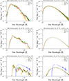 |
Fig. 10. KN spectra comparison between the three different models, generated through the POSSIS code and calculated at 40 Mpc of distance. Each row represents a different time epoch: 0.5 d, 1 d, 1.43 d, respectively. The columns identify different KN ejecta compositions: on the left column, the spectra of panels (a), (c), and (e), are generated by an opacity contribution of 100% of Se. The right columns, (b), (d), and (f), are calculated by considering Se at 10%, and a grey opacity of |

We now look more closely at the spectra at each epoch and focus on the differences between the three models with different Se opacities. Figs. 10a and b show a comparison of the two KN scenarios at texp = 0.5 d. Focusing on the left-hand-side plot, we find that the spectra shape of the three models is similar. On the one hand, the curves show a tail beyond ∼5000 Å, with the highest value about 4 × 10⁻¹⁵ erg s−1 cm−2 Å−1 near 2000 Å. On the other hand, all the three models predict a Se spectral feature in the range of 3000 − 4000 Å. Further differences are also notable between these spectra. The ‘peaks’ do not perfectly overlap, and the absolute intensities vary from spectrum to spectrum. Since we assumed the same modelling criteria, these variations are a consequence of the different opacity inputs adopted in each model. Changing the opacities affects the propagation of photon packets, and consequently the radiation field (Eq. (10)), which in turn influences the temperature (Eq. (9)) and the opacities themselves. An example of this effect is shown in Fig. A.2. These differences in the opacities and the uncertainties in the atomic calculations are reflected in the resulting spectra.
If we now focus on the right-hand plot (Fig. 10b), we see that in a more ‘realistic’ scenario in which Se opacity contributes only 10% of the whole KN mass, the shape of the spectra results in a more regular behaviour with no Se-induced features observable. This is a consequence of Eq. (15). In the previous section, we saw that Se higher opacity is always located in the near-ultraviolet and visibile range, while it becomes almost negligible at large wavelengths, in the near-infrared region. This behaviour is reflected in the spectra. In the wavelength range beyond 2000 Å,  reaches small values such that
  opacity is smaller than
  . Therefore, the grey opacity overwhelms the Se contribution, with no detectable features on the spectra. On the contrary, the slight differences between the models that can be observed at low wavelengths are produced by
  that contributes to exceed the grey opacity. In this case
  becomes greater than
  with the consequence of slight spectra distortion from the continuum shape.
In the epoch texp = 1 d, similar spectra characteristics can be observed. The results are shown in Figs. 10c and d. In general, the left-hand plot shows good agreement between our model (red) and Model I (green) if compared to the Tanaka et al. (2020) model (orange). All three predict a highest intensity value of 6 × 10⁻¹⁶ erg s−1 cm−2 Å−1 at ∼2200 Å, but differ at ∼10 000 Å. Moving to the second scenario, on Fig. 10d no evident discrepancies between the models can be detected, beside the small variations between the plots at low wavelengths, in agreement with the previous analysis.
In the late epoch of texp = 1.43 d, significant differences between the models can be observed. We report them in Figs. 10e and f, together with the uniform reduction and calibration of the X-shooter data for AT2017gfo at the same epoch (Pian et al. 2017; Smartt et al. 2017; Tanvir et al. 2017).
In the left plot, the shapes of the red and green models differ greatly from those of the orange model. In particular, there are absorption features in the ‘Tanaka+,2020’ model that are not there in the other two. In detail, the spectrum calculated with our Se opacity (red) agrees better with the spectrum of Model I (green) generated with the most accurate Se atomic data available. Both spectra show less absorption at 4000 Å and 7000 Å, compared to the model of Tanaka et al. (2020) that predicts a much stronger absorption feature. At 5000 Å, Model I and Tanaka et al. (2020) both provide an intensity ‘peak’ of 10−16 erg s−1 cm−2 Å−1, while, in our model, it is shown at a shifted wavelength position of 6000 Å. These different positions are a direct consequence of the estimate opacity and the accuracy of the atomic calculations.
Finally, a gap in intensity can be noticed between the predicted spectra of the three models and the observed spectrum of AT2017gfo. This difference can be attributed to the over-simplified model of one spherical symmetric component of 10−2 M⊙ assumed in the analysis. In a more realistic scenario, at the epoch of texp = 1.43 d, multiple components of the ejecta with different Ye and a greater total mass of 5 × 10⁻² M⊙ are likely needed to explain the AT2017gfo spectra (Villar et al. 2017; Perego et al. 2017). In addition to the difference in intensity, the modelled spectra are typically bluer than that of AT2017gfo, especially for the case of 100% Se. This effect is driven by the opacities in the 100% Se model being much lower than those expected in KN ejecta and therefore producing spectra that are bluer than those observed (cf. with the photospheric temperature of ∼5000 K estimated for AT2017gfo in Gillanders et al. 2022). The temperature of the 10% Se model is more similar to the observed one. However, the model does not show a strong flux suppression below ∼4000 Å as in AT2017gfo since the adopted grey opacity is only a crude approximation and does not capture the strong line blanketing expected at these phases in these blue wavelength regions (see e.g. Fig. 11 of Tanaka et al. 2020 where the opacity at one day and at these wavelengths can reach ∼10 − 50 cm2 g−1 even for Ye = 0.35).
In the plot of Fig. 10f, we see that all three models perfectly overlap and therefore no possible features of Se can be detected.
6. Selenium atomic opacities in the MARTINI platform
MARTINI is a flexible, user-friendly, open access platform dedicated to astrophysics, in particular to element nucleosynthesis. It combines html pages with a light mysql database, all embedded in the high-level Python Web framework Django. Fig. 11 shows the design and structure of the platform. In detail, all the main topics (e.g. s-process yields, previously available from the FRUITY database website (Cristallo et al. 2011, 2015) and now integrated here, r-process, AGB dust, atomic opacities, KN spectra, and KN light curves) are displayed on the homepage (Fig. 11a). After selecting the field of interest for this article (Atomic-Opacities), a new window is loaded, showing the periodic table of the elements (Fig. 11b). In the periodic table, green buttons represent the available elements with corresponding atomic data, and red buttons represent the in-progress elements, while transparent buttons represent the ones not available yet. Once the element is selected, a new page is shown with all the corresponding ‘.txt’ data files, i.e.: electron configurations, energy levels and transitions for ground and ionised states, opacities and fluxes at various epochs (Fig. 11c). At the top of the page, the general properties together with the corresponding literature references associated with the data of the searched element can be found. Plots of selenium energy levels (compared to NIST ASD) and KN spectra at various epochs (computed with POSSIS) are reported as well.
 |
Fig. 11. Images of the MARTINI platform. Panel (a): homepage of the platform with all the different fields of interest, from s-process to KN light curves. Panel (b): periodic table appearing as intermediate window after the topic selection. Here the user must select one of the available elements (in green) to move to the data page. Panel (c): detailed Se example of the data page. On this page all the literature references, the ‘.txt’ data files, and plots are reported. |
The same scheme will be maintained for the future computation of atomic opacities related to other chemical elements.
7. Conclusions
To investigate and analyse the impact of selenium on KN spectra in the early stage scenario, we performed atomic calculations and opacity estimations for Se I–X ionisation states. We calculated the atomic data using the GRASP2018 code, and compared the results with the NIST ASD and other existing data available from the literature (Tanaka et al. 2020; Radžiūtė & Gaigalas 2022; Kitovienė et al. 2024). Specifically, Se I–IV energy levels deviate ∼5% from the NIST ASD, which results in a significant improvement compared to Tanaka et al. (2020). However, our atomic data do not reach the same accuracy level of Radžiūtė & Gaigalas (2022) and Kitovienė et al. (2024), suggesting that future refinements in atomic calculation are needed. Concerning Se V–VIII, the precision in the calculations is even higher than the Se I–IV results. In detail, Se V and Se VII are ∼2,5%, while Se VI and Se VIII show deviations less than 2%. Since NIST ASD atomic data are not provided for Se IX–X degrees of ionisation, here the reliability of the results only depends on the quality of the level transitions calculated through the classification method described in Kitovienė et al. (2024). The results show a high transition accuracy for ionisation stages beyond Se IV. Taking into account the high quality of these transitions (Fig. 5), together with the high accuracy achieved on the energy levels (Table 5), we provide a robust estimation for Se expansion opacity under the LTE regime. We performed the analysis assuming different temperatures (e.g. T = 5 000 K, T = 10 000 K, T = 20 000 K, and T = 100 000 K). The estimated expansion opacity is calculated with improved accuracy compared to existing works in the literature (e.g. Tanaka et al. 2020). In the last part of the work, we implemented new grids of opacity in the POSSIS code to perform spectral analysis. The grids were calculated using the Se atomic results discussed in Sect. 3.2 and a new set of densities and temperatures, ranging from −19.5 to −4.5 g cm−3 in log-scale and from 1000 to 51 000 K, respectively (see Sect. 5 for more details). In the analysis of the spectra, different KN epochs (e.g. texp = 0.5 d, 1 d, 1.43 d) were investigated, assuming two different scenarios: the first in which the opacity contribution comes from an ejecta made of 100% selenium, and the second in which the opacity of Se only contributes to 10% of the total KN mass, while the rest comes from an adopted grey opacity of 0.5 cm2 g−1. From the results of the KN spectra, Se spectral features can only be observed in the case of 100% of the KN composition, while pushing to a more realistic scenario of 10%, these features are no longer detectable. Finally, all the selenium results discussed in this paper are now available in the new MARTINI platform dedicated to astrophysics, in particular to element nucleosynthesis. These new Se data offer a valuable input to the community to refine future KN models and opacity studies, and they should also be considered for re-investigating previous results.
Acknowledgments
The authors thank the reviewers for their constructive feedback, which significantly improved the clarity and quality of this manuscript. M. Bezmalinovich, D.V. and S.C. acknowledge funding by the European Union – NextGenerationEU RFF M4C2 1.1 PRIN 2022 project ‘2022RJLWHN URKA’ and by INAF 2023 Theory Grant ObFu 1.05.23.06.06. M. Bulla acknowledges the Department of Physics and Earth Science of the University of Ferrara for the financial support through the FIRD 2024 grant. M. Bezmalinovich, D.V. and S.C. are also grateful to S. Simonucci, S. Taioli, T. Morresi, J.H. Gillanders and M. McCann for their support during the work. Finally, the authors acknowledge the support of the PANDORA INFN collaboration.
References
- Abbott, B. P., Abbott, R., Abbott, T. D., et al. 2017a, ApJ, 848, L13 [CrossRef] [Google Scholar]
- Abbott, B. P., Abbott, R., Abbott, T. D., et al. 2017b, ApJ, 848, L12 [Google Scholar]
- Abbott, D. C., & Lucy, L. B. 1985, ApJ, 288, 679 [NASA ADS] [CrossRef] [Google Scholar]
- Andreoni, I., Ackley, K., Cooke, J., et al. 2017, PASA, 34 [Google Scholar]
- Arcavi, I., Hosseinzadeh, G., Howell, D. A., et al. 2017, Nature, 551, 64 [NASA ADS] [CrossRef] [Google Scholar]
- Banerjee, S., Tanaka, M., Kawaguchi, K., Kato, D., & Gaigalas, G. 2020, ApJ, 901, 29 [NASA ADS] [CrossRef] [Google Scholar]
- Banerjee, S., Tanaka, M., Kato, D., et al. 2022, ApJ, 934, 117 [CrossRef] [Google Scholar]
- Banerjee, S., Tanaka, M., Kato, D., & Gaigalas, G. 2024, ApJ, 968, 64 [NASA ADS] [CrossRef] [Google Scholar]
- Bar-Shalom, A., Klapisch, M., & Oreg, J. 2001, JQSRT, 71, 169 [NASA ADS] [CrossRef] [Google Scholar]
- Barnes, J., & Kasen, D. 2013, ApJ, 775, 18 [NASA ADS] [CrossRef] [Google Scholar]
- Barnes, J., Kasen, D., Wu, M.-R., & Martínez-Pinedo, G. 2016, ApJ, 829, 110 [NASA ADS] [CrossRef] [Google Scholar]
- Bezmalinovich, M., Emma, G., Mishra, B., Pidatella, A., & Mascali, D. 2024, Nuovo Cim. C, 47, 1 [Google Scholar]
- Blinnikov, S. I., Eastman, R., Bartunov, O. S., Popolitov, V. A., & Woosley, S. E. 1998, ApJ, 496, 454 [Google Scholar]
- Bulla, M. 2019, MNRAS, 489, 5037 [NASA ADS] [CrossRef] [Google Scholar]
- Bulla, M. 2023, MNRAS, 520, 2558 [CrossRef] [Google Scholar]
- Bulla, M., Sim, S. A., & Kromer, M. 2015, MNRAS, 450, 967 [Google Scholar]
- Busso, M., Gallino, R., & Wasserburg, G. J. 1999, ARA&A, 37, 239 [Google Scholar]
- Carvajal Gallego, H., Deprince, J., Maison, L., Palmeri, P., & Quinet, P. 2024, A&A, 685, A91 [NASA ADS] [CrossRef] [EDP Sciences] [Google Scholar]
- Castor, J. I. 1974, MNRAS, 169, 279 [NASA ADS] [CrossRef] [Google Scholar]
- Chornock, R., Berger, E., Kasen, D., et al. 2017, ApJ, 848, L19 [NASA ADS] [CrossRef] [Google Scholar]
- Corsi, A., Barsotti, L., Berti, E., et al. 2024, Front. Astron. Space Sci., 11 [Google Scholar]
- Cowan, J. J., Sneden, C., Lawler, J. E., et al. 2021, Rev. Mod. Phys., 93, 015002 [Google Scholar]
- Cowperthwaite, P. S., Berger, E., Villar, V. A., et al. 2017, ApJ, 848, L17 [CrossRef] [Google Scholar]
- Cristallo, S., Piersanti, L., Straniero, O., et al. 2011, ApJS, 197, 17 [NASA ADS] [CrossRef] [Google Scholar]
- Cristallo, S., Straniero, O., Piersanti, L., & Gobrecht, D. 2015, ApJS, 219, 40 [Google Scholar]
- De Silva, G. M., Freeman, K. C., Bland-Hawthorn, J., et al. 2015, MNRAS, 449, 2604 [NASA ADS] [CrossRef] [Google Scholar]
- Dessart, L., & Hillier, D. J. 2005, A&A, 439, 671 [NASA ADS] [CrossRef] [EDP Sciences] [Google Scholar]
- Domoto, N., Tanaka, M., Kato, D., et al. 2022, ApJ, 939, 8 [NASA ADS] [CrossRef] [Google Scholar]
- Drout, M. R., Piro, A. L., Shappee, B. J., et al. 2017, Science, 358, 1570 [NASA ADS] [CrossRef] [Google Scholar]
- Eastman, R. G., & Pinto, P. A. 1993, ApJ, 412, 731 [NASA ADS] [CrossRef] [Google Scholar]
- Evans, P. A., Cenko, S. B., Kennea, J. A., et al. 2017, Science, 358, 1565 [NASA ADS] [CrossRef] [Google Scholar]
- Fischer, C. F., Godefroid, M., Brage, T., Jönsson, P., & Gaigalas, G. 2016, J. Phys. B, 49, 182004 [Google Scholar]
- Flörs, A., Silva, R. F., Deprince, J., et al. 2023, MNRAS, 524, 3083 [CrossRef] [Google Scholar]
- Fontes, C. J., Fryer, C. L., Hungerford, A. L., Wollaeger, R. T., & Korobkin, O. 2020, MNRAS, 493, 4143 [CrossRef] [Google Scholar]
- Fontes, C. J., Fryer, C. L., Wollaeger, R. T., Mumpower, M. R., & Sprouse, T. M. 2023, MNRAS, 519, 2862 [Google Scholar]
- Froese Fischer, C., Gaigalas, G., Jönsson, P., & Bieroń, J. 2019, Comput. Phys. Commun., 237, 184 [NASA ADS] [CrossRef] [Google Scholar]
- Gaigalas, G., Fritzsche, S., & Grant, I. P. 2001a, Comput. Phys. Commun., 139, 263 [NASA ADS] [CrossRef] [Google Scholar]
- Gaigalas, G., Zalandauskas, T., & Rudzikas, Z. 2001b, Lith. J. Phys., 41, 226 [Google Scholar]
- Gaigalas, G., Žalandauskas, T., & Rudzikas, Z. 2003, At. Data Nucl. Data Tables, 84, 99 [Google Scholar]
- Gaigalas, G., Fischer, C., Rynkun, P., & Jönsson, P. 2017, Atoms, 5, 6 [CrossRef] [Google Scholar]
- Gaigalas, G., Zalandauskas, T., & Fritzsche, S. 2004, Comput. Phys. Commun., 157, 239 [Google Scholar]
- Gallino, R., Arlandini, C., Busso, M., et al. 1998, ApJ, 497, 388 [Google Scholar]
- Gillanders, J. H., McCann, M., Sim, S. A., Smartt, S. J., & Ballance, C. P. 2021, MNRAS, 506, 3560 [NASA ADS] [CrossRef] [Google Scholar]
- Gillanders, J. H., Smartt, S. J., Sim, S. A., Bauswein, A., & Goriely, S. 2022, MNRAS, 515, 631 [NASA ADS] [CrossRef] [Google Scholar]
- Grant, I. P. 2007, Relativistic Quantum Theory of Atoms and Molecules (New York: Springer) [Google Scholar]
- Guiglion, G., Battistini, C., Bell, C. P. M., et al. 2019, The Messenger, 175, 17 [NASA ADS] [Google Scholar]
- Hauschildt, P. H., & Baron, E. 1999, J. Comput. Appl. Math., 109, 41 [NASA ADS] [CrossRef] [Google Scholar]
- He, X.-B., Thomas Tam, P.-H., & Shen, R.-F. 2018, Res. Astron. Astrophys., 18, 043 [Google Scholar]
- Höeflich, P., Müeller, E., & Khokhlov, A. 2021, A&A, 268, 570 [Google Scholar]
- Jin, S., Trager, S. C., Dalton, G. B., et al. 2024, MNRAS, 530, 2688 [NASA ADS] [CrossRef] [Google Scholar]
- Karp, A. H., Lasher, G., Chan, K. L., & Salpeter, E. E. 1977, ApJ, 214, 161 [NASA ADS] [CrossRef] [Google Scholar]
- Kasen, D., & Barnes, J. 2019, ApJ, 876, 128 [Google Scholar]
- Kasen, D., Thomas, R. C., & Nugent, P. 2006, ApJ, 651, 366 [NASA ADS] [CrossRef] [Google Scholar]
- Kasen, D., Badnell, N. R., & Barnes, J. 2013, ApJ, 774, 25 [NASA ADS] [CrossRef] [Google Scholar]
- Kasen, D., Fernández, R., & Metzger, B. D. 2015, MNRAS, 450, 1777 [NASA ADS] [CrossRef] [Google Scholar]
- Kasen, D., Metzger, B., Barnes, J., Quataert, E., & Ramirez-Ruiz, E. 2017, Nature, 551, 80 [Google Scholar]
- Kasliwal, M. M., Nakar, E., Singer, L. P., et al. 2017, Science, 358, 1559 [NASA ADS] [CrossRef] [Google Scholar]
- Kato, D. I., Tanaka, M., et al. 2021, Japan-Lithuania Opacity Database for Kilonova [Google Scholar]
- Kato, D., Tanaka, M., Gaigalas, G., Kitovienė, L., & Rynkun, P. 2024, MNRAS, 535, 2670 [Google Scholar]
- Kerzendorf, W. E., & Sim, S. A. 2014, MNRAS, 440, 387 [NASA ADS] [CrossRef] [Google Scholar]
- Kitovienė, L., Gaigalas, G., Rynkun, P., Tanaka, M., & Kato, D. 2024, J. Phys. Chem. Ref. Data, 53 [Google Scholar]
- Kramida, A., & Ralchenko, Y. 1999, NIST Atomic Spectra Database [Google Scholar]
- Kromer, M., & Sim, S. A. 2009, MNRAS, 398, 1809 [Google Scholar]
- Lucy, L. B. 2003, A&A, 403, 261 [NASA ADS] [CrossRef] [EDP Sciences] [Google Scholar]
- Lyman, J. D., Lamb, G. P., Levan, A. J., et al. 2018, Nat. Astron., 2, 751 [NASA ADS] [CrossRef] [Google Scholar]
- Majewski, S. R., Schiavon, R. P., Frinchaboy, P. M., et al. 2017, AJ, 154, 94 [NASA ADS] [CrossRef] [Google Scholar]
- Mascali, D., Santonocito, D., Amaducci, S., et al. 2022, Universe, 8, 80 [CrossRef] [Google Scholar]
- Mazzali, P. A., & Lucy, L. B. 1993, A&A, 279, 447 [NASA ADS] [Google Scholar]
- McCully, C., Hiramatsu, D., Howell, D. A., et al. 2017, ApJ, 848, L32 [NASA ADS] [CrossRef] [Google Scholar]
- Metzger, B. D. 2019, Liv (Relat.: Rev), 23 [Google Scholar]
- Nedora, V., Bernuzzi, S., Radice, D., et al. 2019, ApJ, 886, L30 [NASA ADS] [CrossRef] [Google Scholar]
- Perego, A., Radice, D., & Bernuzzi, S. 2017, ApJ, 850, L37 [NASA ADS] [CrossRef] [Google Scholar]
- Perego, A., Vescovi, D., Fiore, A., et al. 2022, ApJ, 925, 22 [CrossRef] [Google Scholar]
- Pian, E., D’Avanzo, P., Benetti, S., et al. 2017, Nature, 551, 67 [Google Scholar]
- Pidatella, A., Cristallo, S., Galatá, A., et al. 2021, Nuovo Cim. C, 44, 1 [Google Scholar]
- Pignatari, M., Gallino, R., Heil, M., et al. 2010, ApJ, 710, 1557 [Google Scholar]
- Pognan, Q., Jerkstrand, A., & Grumer, J. 2022, MNRAS, 513, 5174 [NASA ADS] [CrossRef] [Google Scholar]
- Prantzos, N., Abia, C., Cristallo, S., Limongi, M., & Chieffi, A. 2020, MNRAS, 491, 1832 [Google Scholar]
- Radice, D., Bernuzzi, S., & Perego, A. 2020, Annu. Rev. Nucl. Part. Sci., 70, 95 [Google Scholar]
- Radžiūtė, L., & Gaigalas, G. 2022, At. Data Nucl. Data Tables, 147, 101515 [Google Scholar]
- Randich, S., Gilmore, G., Magrini, L., et al. 2022, A&A, 666, A121 [NASA ADS] [CrossRef] [EDP Sciences] [Google Scholar]
- Rosswog, S., & Korobkin, O. 2024, Ann. Phys., 536 [Google Scholar]
- Rybicki, G. B., & Lightman, A. P. 1979, Radiative Processes in Astrophysics (New York: Wiley) [Google Scholar]
- Shingles, L. J., Collins, C. E., Vijayan, V., et al. 2023, ApJ, 954, L41 [NASA ADS] [CrossRef] [Google Scholar]
- Smartt, S. J., Chen, T.-W., Jerkstrand, A., et al. 2017, Nature, 551, 75 [Google Scholar]
- Sneppen, A., & Watson, D. 2023, A&A, 675, A194 [NASA ADS] [CrossRef] [EDP Sciences] [Google Scholar]
- Sneppen, A., Watson, D., Gillanders, J. H., & Heintz, K. E. 2024, A&A, 688, A95 [NASA ADS] [CrossRef] [EDP Sciences] [Google Scholar]
- Soares-Santos, M., Holz, D. E., Annis, J., et al. 2017, ApJ, 848, L16 [CrossRef] [Google Scholar]
- Sobolev, V. V. 1960, Moving Envelopes of Stars (Harvard: Harvard University Press) [Google Scholar]
- Straniero, O., Gallino, R., & Cristallo, S. 2006, Nucl. Phys. A, 777, 311 [NASA ADS] [CrossRef] [Google Scholar]
- Tanaka, M., & Hotokezaka, K. 2013, ApJ, 775, 113 [NASA ADS] [CrossRef] [Google Scholar]
- Tanaka, M., Kato, D., Gaigalas, G., & Kawaguchi, K. 2020, MNRAS, 496, 1369 [NASA ADS] [CrossRef] [Google Scholar]
- Tanvir, N. R., Levan, A. J., González-Fernández, C., et al. 2017, ApJ, 848, L27 [CrossRef] [Google Scholar]
- Utrobin, V. P. 2004, Astron. Lett., 30, 293 [NASA ADS] [CrossRef] [Google Scholar]
- Utsumi, Y., Tanaka, M., Tominaga, N., et al. 2017, PASJ, 69 [Google Scholar]
- Vescovi, D., Reifarth, R., Cristallo, S., & Couture, A. 2022, Front. Astron. Space Sci., 9 [Google Scholar]
- Villar, V. A., Guillochon, J., Berger, E., et al. 2017, ApJ, 851, L21 [Google Scholar]
- Watson, D., Hansen, C. J., Selsing, J., et al. 2019, Nature, 574, 497 [NASA ADS] [CrossRef] [Google Scholar]
- Wollaeger, R. T., & van Rossum, D. R. 2014, ApJS, 214, 28 [NASA ADS] [CrossRef] [Google Scholar]
- Wollaeger, R. T., Korobkin, O., Fontes, C. J., et al. 2018, MNRAS, 478, 3298 [NASA ADS] [CrossRef] [Google Scholar]
We note that using different inputs for heating rates and opacities and decoupling them through their dependence on Ye may break self-consistency. In the future, we plan to carry out simulations where heating rates and opacities are computed self-consistently for specific compositions of the ejecta.
Appendix A: Additional figures
 |
Fig. A.1. Se I–X expansion opacity at T = 100 000 K. In the panels, it can be seen that the opacity contribution at T = 100 000 K only comes from the ionisation stages beyond Se VI. No significant contribution can be observed in the ionisation stages between Se I–VI. |
 |
Fig. A.2. Density, temperature, opacity and optical depth (from left to right) maps in the yz plane for the model with 100% Se (upper panels) and 10% Se (lower panels). The white circles show the location of the thermalisation/photospheric surface, and the value of its temperature is indicated in the corresponding panels. Maps are computed at 1 d after the merger. Note that the colour bars of the upper and lower panels have the same ranges, except for those of the opacities κ. |
All Tables
All Figures
|
Fig. 1. Abundances of light r-process elements for trajectories representative of the dynamical polar wind and spiral-wave wind, at 1.5 days after merger. For both trajectories, selenium accounts for about 10% of the total mass. |
| In the text | |
|
Fig. 2. Se I–IV energy levels of the four works compared with the NIST ASD. In the analysis we considered all energy levels below ionisation for each state. The dashed lines represent the ionisation threshold for each ionisation degree. |
| In the text | |
|
Fig. 3. Se ionisation fraction as a function of the temperature. Vertical dashed lines indicate the temperature at which a new ionisation state is rising. The blue panel represents the range of temperatures of interest for the early stage KN (≳10 000 K). |
| In the text | |
|
Fig. 4. Se V–X energy levels of our GRASP2018 atomic calculations compared with the NIST ASD. In the analysis we considered all energy levels below ionisation for each state. The dashed lines represent the ionisation threshold for each ionisation degree. |
| In the text | |
|
Fig. 5. Se I–X transition classes of GRASP2018 calculation. In the legend, ‘AA’ denotes transitions computed with highly accurate wave functions, whereas ‘E’ indicates the least accurate ones. |
| In the text | |
|
Fig. 6. Se II–III transition classes of our GRASP2018 atomic calculations compared with Radžiūtė & Gaigalas (2022) Se II, and Kitovienė et al. (2024) Se III. |
| In the text | |
|
Fig. 7. Comparison of Se I–IV expansion opacity at T = 5000 K calculated with the three different sets of atomic data. Each banner corresponds to the expansion opacity calculated with the specific set of atomic data. In the top panel the opacity is calculated considering Se I–IV data from this work. In the middle panel the opacity is calculated considering Se I–IV data from Model I. In the bottom panel the opacity is calculated considering Se I–IV data from ‘Tanaka+,2020’. In the plot legend, the notation ‘I–II’, ‘I–III’, and ‘I–IV’ indicates that the opacity is calculated by including time-by-time additional ionisation states. |
| In the text | |
|
Fig. 8. Comparison of Se I–IV expansion opacity at T = 10 000 K calculated with the three different sets of atomic data. Each banner corresponds to the expansion opacity calculated with the specific set of atomic data. In the top panel the opacity is calculated considering Se I–IV data from this work. In the middle panel the opacity is calculated considering Se I–IV data from Model I. In the bottom panel the opacity is calculated considering Se I–IV data from model ‘Tanaka+,2020’. In the plot legend, the notation ‘I–II’, ‘I–III’, and ‘I–IV’ indicates that the opacity is calculated by including time-by-time additional ionisation states. |
| In the text | |
|
Fig. 9. Comparison of Se I–X expansion opacity at T = 20 000 K calculated with Se I–X data presented in this work. In the plot legend, the notation ‘I–X’ indicates that the opacity is calculated by including all the ionisation states from ‘I’ to ‘X’. At the top panel of (a), we show a comparison between the Se I–X and Se I–V ionisation states, while in the bottom panel we present the different ionisation state contribution from Se I to Se X. Panel (b): same analysis with a zoomed-in view in the wavelength range 0–5000 Å. From both figures, we see that only the ionisation degrees between Se III and Se V matter for the opacity calculation at T = 20 000 K. |
| In the text | |
|
Fig. 10. KN spectra comparison between the three different models, generated through the POSSIS code and calculated at 40 Mpc of distance. Each row represents a different time epoch: 0.5 d, 1 d, 1.43 d, respectively. The columns identify different KN ejecta compositions: on the left column, the spectra of panels (a), (c), and (e), are generated by an opacity contribution of 100% of Se. The right columns, (b), (d), and (f), are calculated by considering Se at 10%, and a grey opacity of |
| In the text | |
|
Fig. 11. Images of the MARTINI platform. Panel (a): homepage of the platform with all the different fields of interest, from s-process to KN light curves. Panel (b): periodic table appearing as intermediate window after the topic selection. Here the user must select one of the available elements (in green) to move to the data page. Panel (c): detailed Se example of the data page. On this page all the literature references, the ‘.txt’ data files, and plots are reported. |
| In the text | |
|
Fig. A.1. Se I–X expansion opacity at T = 100 000 K. In the panels, it can be seen that the opacity contribution at T = 100 000 K only comes from the ionisation stages beyond Se VI. No significant contribution can be observed in the ionisation stages between Se I–VI. |
| In the text | |
|
Fig. A.2. Density, temperature, opacity and optical depth (from left to right) maps in the yz plane for the model with 100% Se (upper panels) and 10% Se (lower panels). The white circles show the location of the thermalisation/photospheric surface, and the value of its temperature is indicated in the corresponding panels. Maps are computed at 1 d after the merger. Note that the colour bars of the upper and lower panels have the same ranges, except for those of the opacities κ. |
| In the text | |
Current usage metrics show cumulative count of Article Views (full-text article views including HTML views, PDF and ePub downloads, according to the available data) and Abstracts Views on Vision4Press platform.
Data correspond to usage on the plateform after 2015. The current usage metrics is available 48-96 hours after online publication and is updated daily on week days.
Initial download of the metrics may take a while.