| Issue |
A&A
Volume 696, April 2025
|
|
|---|---|---|
| Article Number | A32 | |
| Number of page(s) | 30 | |
| Section | Atomic, molecular, and nuclear data | |
| DOI | https://doi.org/10.1051/0004-6361/202452967 | |
| Published online | 01 April 2025 | |
Kilonova ejecta opacity inferred from new large-scale HFR atomic calculations in all elements between Ca (Z = 20) and Lr (Z = 103)
1
Atomic Physics and Astrophysics, Université de Mons (UMONS),
Mons,
Belgium
2
Astronomy and Astrophysics Institute, Université Libre de Bruxelles,
Brussels,
Belgium
3
Spectroscopy, Quantum Chemistry and Atmospheric Remote Sensing, Université Libre de Bruxelles,
Brussels,
Belgium
4
GSI Helmholtzzentrum für Schwerionenforschung,
Darmstadt,
Germany
5
Astrophysical Big Bang Laboratory, RIKEN Cluster for Pioneering Research,
Wako,
Japan
6
IPNAS, ULiège,
Liège,
Belgium
★ Corresponding author; This email address is being protected from spambots. You need JavaScript enabled to view it.
Received:
12
November
2024
Accepted:
16
February
2025
Abstract
Context. The production of elements heavier than iron in the Universe still remains an unsolved mystery. About half of them are thought to be produced by the astrophysical r-process (rapid neutron-capture process), for which neutron star mergers (NSMs) are among the most promising production sites. In August 2017, gravitational waves generated by a NSM were detected for the first time by the LIGO detectors (event GW170817), and the observation of its electromagnetic counterpart, the kilonova (KN) AT2017gfo, suggested the presence of heavy elements in the KN ejecta. The luminosity and spectra of such KN emission depend significantly on the ejecta opacity. Atomic data and opacities for heavy elements are thus sorely needed to model and interpret KN light curves and spectra.
Aims. The present work focuses on large-scale atomic data and opacity computations for all heavy elements with Z ≥ 20, with a special effort on lanthanides and actinides, for a grid of typical KN ejecta conditions (temperature, density, and time post-merger) between one day and one week after the merger (corresponding to the local thermodynamical equilibrium photosphere phase of the KN ejecta).
Methods. In order to do so, we used the pseudo-relativistic Hartree–Fock (HFR) method as implemented in Cowan’s codes, in which the choice of the interaction configuration model is of crucial importance.
Results. In this paper, HFR atomic data and opacities for all elements between Ca (Z = 20) and Lr (Z = 103) are presented, with a special focus on lanthanides and actinides. In particular, we found increased lanthanide opacities compared to previous works. Besides, we also discuss the contribution of every single element with Z ≥ 20 to the total KN ejecta opacity for a given NSM model, depending on their Planck mean opacities and elemental abundances. An important result is that lanthanides are found to not be the dominant sources of opacity, at least on average. The impact on KN light curves of considering such atomic-physics-based opacity data instead of typical crude approximation formulae is also evaluated. In addition, the importance of taking the ejecta composition into account directly in the expansion opacity determination (instead of estimating single-element opacities) is highlighted. A database containing all the relevant atomic data and opacity tables has also been created and published online along with this work.
Key words: atomic data / atomic processes / nuclear reactions, nucleosynthesis, abundances / opacity / radiative transfer / stars: neutron
© The Authors 2025
 Open Access article, published by EDP Sciences, under the terms of the Creative Commons Attribution License (https://creativecommons.org/licenses/by/4.0), which permits unrestricted use, distribution, and reproduction in any medium, provided the original work is properly cited.
This article is published in open access under the Subscribe to Open model. This email address is being protected from spambots. You need JavaScript enabled to view it. to support open access publication.
1 Introduction
The stable neutron-rich nuclides heavier than iron observed in stars of various metallicities and in the solar system are produced by the rapid neutron-capture process (or r-process) of stellar nucleosynthesis. The r-process is responsible for creating about half of the atomic nuclei heavier than iron. This process occurs in explosive environments with extremely high neutron densities and temperatures (Arnould et al. 2007; Arnould & Goriely 2020; Cowan et al. 2021). The exact astrophysical sites of the r-process have been extensively searched for. For a long time, core-collapse supernovae of massive stars were considered the primary r-process sites, but so far no successful r-process has been found in the most sophisticated models (e.g. Janka 2017; Wanajo et al. 2018; Wang & Burrows 2023, and references therein). Collapsars, a subclass of core-collapse supernovae corresponding to rapidly rotating and highly magnetized massive stars and associated with the origin of observed long γ-ray bursts, remain promising r-process sites (Winteler et al. 2012; Siegel et al. 2019; Miller et al. 2019; Just et al. 2022). Alternatively, neutron star (NS) mergers have been also envisioned as a potential site for the r-process (Lattimer & Schramm 1974; Eichler et al. 1989). Hydrodynamical simulations of NS mergers have confirmed that a considerable amount of matter could be ejected from these systems (e.g. Ruffert et al. 1996; Rosswog et al. 1999). Associated nucleosynthesis calculations have shown that NS mergers are viable r-process sites (see e.g. Goriely et al. 2011; Korobkin et al. 2012; Wanajo et al. 2014; Just et al. 2015, 2023; Radice et al. 2018; Kullmann et al. 2023). The resulting abundance distributions are found to reproduce remarkably well the solar system distribution, as well as various elemental distributions observed in low-metallicity stars. In addition, the ejected mass of r-process material, combined with the predicted astrophysical event rate (around 10 My−1 in the Milky Way) can account for the majority of r-process material in our Galaxy. Another piece of evidence that NS mergers are major contributors to the Galactic r-process-enrichment comes from the remarkable 2017 gravitational wave event GW170817 (Abbott et al. 2017a) and its electromagnetic counterpart AT 2017gfo (Abbott et al. 2017b). The decay of freshly produced radioactive r-process elements is expected to power such a kilonova (KN), which is potentially observable in the optical and (near-)infrared electromagnetic spectrum. Fits to the observed KN light curve provide a strong indication that r-process elements were synthesized in this event (e.g. Kasen et al. 2017). Watson et al. (2019); Gillanders et al. (2022) also report the spectroscopic identification of Sr (Z = 38), providing the first direct evidence that NS mergers eject material enriched in heavy elements.
The light curve of a KN delivers unique information about the ejecta mass and velocity, and its composition. However, the modeling of these merger events and the resulting KN explosion still faces considerable challenges, including in particular the description of radiative processes that determine the opacity and emission observed. This requires the most complete knowledge possible of atomic data such as energy levels, transition wavelengths, and oscillator strengths characterizing the species contributing to the opacity. A major effort has been made in this direction in recent years with various studies aimed at determining the relevant atomic parameters and deducing the corresponding opacity for many heavy elements. Among these studies, we mention the works published by Tanaka et al. (2020) for elements ranging from Fe to Ra in ionization stages from I to IV, by Fontes et al. (2020, 2023) for all lanthanide and actinide atoms in charge stages between I and IV, by Banerjee et al. (2022) for three selected lanthanides (i.e., Nd, Sm, and Eu) from V to XI, and by Banerjee et al. (2024) for all elements from La to Ra in the charge stages ranging from I to XI, to which must be added investigations more focused on specific elements such as the works published by Gaigalas et al. (2022) for Pr IV, Gaigalas et al. (2019) for Nd II–IV, Gaigalas et al. (2020) and Deprince et al. (2024) for Er III, Radžiūtė et al. (2020) for Pr II–Gd II, Radžiūtė et al. (2021) for Tb II–Yb II, Carvajal Gallego et al. (2021) for Ce II–IV, Rynkun et al. (2022) for Ce IV, Carvajal Gallego et al. (2022a) for Ce V–X, Carvajal Gallego et al. (2022b) for La V–X, Carvajal Gallego et al. (2023a) for Pr V–X, Nd V–X, and Pm V–X, Carvajal Gallego et al. (2023c) for Sm V–X, Maison et al. (2022) for Lu V, Ben Nasr et al. (2023) for Nb I–IV and Ag I–IV, Ben Nasr et al. (2024) for Hf I–IV, Os I–IV, and Au I–IV, Deprince et al. (2023) for U II–III, and Flörs et al. (2023) for Nd II–III and U II–III. We also add to all these investigations the recent paper published by Peng et al. (2024) concerning KN light curve interpolation with neural networks.
In the present work, we report new opacity calculations for all elements with 20 ≤ Z ≤ 103 (i.e., from Ca to Lr), using a consistent set of atomic parameters obtained with the pseudo- relativistic Hartree–Fock (HFR) method for all atomic species of interest in the first four charge states (I–IV). A comparison with the most complete previous works is also discussed, as well as the impact on KN light curve models.
In Sect. 2, the HFR method is described, as well as the atomic models used for each ion considered in this work. A discussion about the accuracy of our atomic data is also carried out. The expansion opacities of all elements from Ca to Lr are illustrated for typical KN ejecta conditions in Sect. 3, as well as a comparison with a similar previous work. The same type of comparison is performed in Sect. 4 concerning the Planck mean line-binned opacities. In Sect. 5, we introduce and detail the new HFR atomic database and opacity tables produced in this work and available online. Finally, in Sect. 6, the impact of the newly calculated HFR opacities is illustrated in the case of a NS merger simulation. Special attention is paid to the elements contributing the most to the ejecta opacity and to their impact on the light curve in comparison with alternative approximations.
2 HFR computations
The pseudo-Relativistic Hartree-Fock code (HFR) was developed by Cowan (1981). In this method, a set of orbitals is obtained for each configuration by solving the Hartree– Fock (HF) equations that are derived from the application of the variational principle on the corresponding configuration average energy. In addition, several relativistic corrections are included in a perturbative way; namely, the Blume-Watson spin–orbit (including the one-body Breit interaction operator), mass-velocity, and one-body Darwin terms. The coupled HF equations are solved by using the self-consistent field approach.
Within the framework of the Slater–Condon method, the atomic wavefunctions (eigenfunctions of the Hamiltonian) are built as a superposition of basis wavefunctions in the LS Jπ representation; that is,
 (1)
(1)
The construction and diagonalization of the multiconfiguration Hamiltonian matrix are carried out within the framework of the Slater-Condon theory. Each matrix element is computed as a sum of products of Racah angular coefficients  , and radial Slater and spin-orbit integrals (xl):
 (2)
(2)
As was recommended by Cowan (1981), scaling factors of 0.85 were applied to the Slater integrals in the present calculations. The choice of scaling factors between 0.8 and 0.95 virtually does not affect the computed expansion opacities, as was recently shown by Carvajal Gallego et al. (2023a) in the case of Nd IX.
The radiative transition wavelengths and oscillator strengths for each transition allowed in the electric dipole approximation can then be computed from the eigenvalues and eigenstates obtained using such approach. It should be noted that only the transitions characterized by log gf ≥ −5 are considered in this work, since it was shown by Carvajal Gallego et al. (2022a) that values under this cutoff do not modify the computed expansion opacity.
For all lanthanide and actinide ions considered in this work, namely from the neutral to the trebly ionized species, the same methodology was adopted to build the multiconfiguration models, considering single and double electron substitutions from reference configurations. In more detail, for all the lanthanides, the model for each ion was built by considering single electron excitations from the ground configuration toward all n = 5 and n = 6 orbitals, as well as configurations arising from double excitations from the ground one to selected n = 5 and n = 6 orbitals, namely 5d, 6s, and 6p, with a few isolated restrictions for ions characterized by an atomic structure with a very large number of states (and thus by a very large Hamiltonian matrix to be diagonalized). Similarly, for actinides, the same single and double excitations to the corresponding n = 6 and n = 7 orbitals were considered (i.e., all the single electron substitutions from the ground configuration to n = 6 and n = 7 orbitals as well as double excitations toward 6d, 7s, and 7p). The lists of the configurations included in our models are given in Table A.1. The justification of such model choices is based on the same strategy that we used for Nd II, Nd III, U II, and U III in Flörs et al. (2023), in which we show that the resulting HFR atomic data lead to converged expansion opacities. The accuracy of the atomic data obtained for Nd II, Nd III, U II, and U III has already been discussed in Flörs et al. (2023). In summary, in this paper, we compared our HFR atomic levels with the ones computed by another independent method, namely the Flexible Atomic Code (FAC) (Gu 2008), and found an overall agreement between 10% and 20% for these four ions. When compared to experimental energy levels from the pioneer compilation of Blaise & Wyart (1992) entitled “Selected Constants Energy Levels and Atomic Spectra of Actinides” (abbreviated as SCASA and available in an online database (Blaise & Wyart 1994)), our HFR energy levels agree within 18% to 30%, except for Nd III, for which a larger discrepancy was obtained (49%), doing in some cases worse and in other cases better than the FAC computations depending on the ion. We also used the same strategy to build the HFR multiconfiguration model of Er III in the same context in Deprince et al. (2024), for which an overall agreement of 37% was found when comparing our energy levels with experimental data from Wyart et al. (1997). We showed in Deprince et al. (2023) and Deprince et al. (2024) that, even if a non-negligible discrepancy was obtained between our HFR atomic levels and experimental data for U II, U III, and Er III, a calibration of our data consisting in fitting the computed configuration average energies to the ones deduced from SCASA (Blaise & Wyart 1994) and from Wyart et al. (1997) greatly improves the accuracy of our energy levels (e.g., the overall agreement was reduced from 37% to 4% in the case of Er III, see Deprince et al. 2024) but has only a minor impact on the expansion opacities. In particular, the ground levels computed without calibration do not match the observed ones for those three ions (which is the case for 23 ions among all the 120 lanthanide and actinides ions considered in this work). However, as was mentioned above, we observed that the expansion opacities were virtually unaffected by the level inversion calibration and concluded that, in the framework of large-scale computations of atomic data for opacity determination, this calibration could be omitted – at least in a first step – for ions with high spectral densities as lanthanides and actinides and for the conditions expected in KN ejecta (Deprince et al. 2023, 2024).
For all the other elements from Z = 20 (i.e., 20 ≤ Z ≤ 56 and 72 ≤ Z ≤ 88), namely those belonging to the fourth, fifth, sixth, and seventh rows of the periodic table, we also considered all the neutrals and ions up to IV ionization stage.
Firstly, we focus on the elaboration of the configuration lists for the fourth row transition metal elements, namely those with an open 3d subshell. For Co I and the corresponding isoelectronic fourth row ions (namely Ni II, Cu III, and Zn IV), which are all homologous to Ag III, we used a configuration interaction (CI) model of the same type as the one used in our paper Ben Nasr et al. (2023); that is, with an [Ar] core instead of a [Kr] core and 3d up to 6f valence orbitals instead of 4d up to 8f valence orbitals. For the other neutral fourth row elements and their isoelectronic ions, the same list of configurations as for Co I were considered increasing or decreasing the number of electrons in the 3d subshell. For Sc IV and the corresponding isoelectronic fourth row transition metal Ti V, single excitations of 3p electron from the 3p6 configuration to valence subshells up to 6f were used to generate the list of configurations. As far as calcium ions are considered, for Ca I, all single excitations of an electron 4s from the ground configuration 4s2 to the valence subshells up to 6f were used to build the CI list, which was further extended by adding the 3d2 and 4p2 configurations. Concerning the other ions, namely Ca II, Ca III, and Ca IV, which are, respectively, isoelectronic to Sc III, Sc IV, and Sc V, the same lists of interacting configurations were thus considered, except for Ca IV, for which the configuration 3s3p6 was added in the list. The fourth row elements from Z = 31 to Z = 36 are characterized by the filling of the 4p subshell. For Ga I, single excitations of the 4p electron from the ground configuration 4s24p to the valence orbitals up to 6f were considered to build the CI model in a first step. The list was then extended by adding the 4s4p2, 4s4p5s, 4s4p4d, and 4p3 configurations. For all the other neutral species, the lists of interacting configurations were deduced by gradually filling the 4p subshell from the Ga I CI model. Regarding the other ionization stages, the CI lists were deduced from the corresponding isoelectronic sequence of each ion (e.g., since Ge II, As III, and Se IV correspond to the isoelectronic sequence of Ga, we used the same multiconfiguration model for these ions).
Concerning the fifth-row elements (Z = 37–54), the lists of interacting configurations included in the various models were deduced from the corresponding fourth-row homologous ions (Z = 20–36), besides the neutral rubidium (since we considered elements from Z = 20 for the fourth row), whose CI list was generated by considering single excitation of the 5s electron from the ground configuration 5s to valence subshells up to 7f. The same approach was also used to build the multiconfiguration models of the sixth-row elements (Z = 72–86) as well as for cesium (Z = 55), barium (Z = 56), francium (Z = 87), and radium (Z = 88); that is, the configuration lists were built based on the homologous fifth-row element ones.
The configuration models used for all the elements considered in this work (i.e., elements with 20 ≤ Z ≤ 103) are presented in Table A.1.
3 Expansion opacity
We computed the bound-bound opacities of all the elements mentioned in Section 2 for typical conditions expected in the KN ejecta (roughly guided by the AT2017gfo case) from 1 to 7 days after the NSM which corresponds to the photosphere phase of the KN, in which local thermodynamical equilibrium (LTE) conditions are expected to be valid (Pognan et al. 2022). From roughly one week post-merger, non-LTE (NLTE) effects are expected to be more important. In this study, we thus limit ourselves to the KN photosphere phase from 1 day after the merger. The corresponding conditions of temperature and density within the KN ejecta can be estimated from ejecta distributions resulting in hydrodynamical simulations, as is illustrated in Fig. 1 showing the temperature and density conditions expected in the photosphere of the KN ejecta of a 1.375–1.375 M⊙ NS merger (model “sym-n1-a6” in Just et al. 2023) from t = 0.1 d until the ejecta becomes optically thin, and for which we adopted the heuristic prescription described in Just et al. (2022) for the opacity and photosphere. Based on these estimates, we computed the atomic opacities of all the elements between Z = 20 and Z = 103 for a grid of conditions corresponding to temperatures of 1000 K ≤ T ≤ 10 000 K and densities of 10−17 g cm−3 ≤ ρ ≤ 10−13 g cm−3. For such temperatures, only the low-ionization stages of the elements are present in the KN ejecta; namely, from the neutral to the trebly ionized species (see e.g., Tanaka et al. 2020; Flörs et al. 2023). We thus focus our work on these ions, which were already mentioned in Section 2. As in previous studies (e.g., Flörs et al. 2023; Tanaka et al. 2020), the opacities given in this section (as well as in Section 4) serve as an illustration and a means of comparison with data provided by other groups since they adopt a composition with 100% of a given element, which is unrealistic since the KN ejecta total opacity obviously depends on the elemental abundance pattern resulting from r-process nucleosynthesis. More realistic opacities based on ejecta compositions deduced from astrophysical simulations will be discussed in Section 6.
In this study, we mainly focus on the widely used expansion opacity (see Eastman & Pinto 1993; Kasen et al. 2013; Tanaka & Hotokezaka 2013) defined as
 (3)
(3)
where t is the time after the merger, ρ is the ejecta density, ∆λ is the wavelength bin width, and λl is the transition wavelength with Sobolev optical depth
 (4)
(4)
in which fl is the oscillator strength of the line with transition wavelength λl and the corresponding lower level number density, nl . The number densities of the lower levels can be computed under the LTE assumption by using the Saha ionization balance,
 (5)
(5)
and Boltzmann population equations,
 (6)
(6)
where Ni and nk, respectively, correspond to the ion population and the level population, Ui(T) is the partition function, ne is the electron density, λdB is the thermal de Broglie wavelength, Eion is the ionization energy, gk is the multiplicity of the level (2 Jk + 1), and Ek is the level energy.
In this work, the bin width was chosen to be 1% of the wavelength, but it is worth mentioning that neither the absolute scale nor the general shape of the expansion opacity depends on the bin width, as has been mentioned for example by Flörs et al. (2023). In the literature, a bin width of 10 Å is often assumed, but our choice results in smoother (and therefore easier to read) curves. The choice of using the Sobolev approximation (Sobolev 1960) to compute opacities in the expansion formalism is justified for NS merger ejecta (see e.g., Flörs et al. 2023) by the high expansion velocities (∼0.1c) of the ejecta.
The opacity thus depends on the physical conditions within the ejecta for a given time post merger; that is, the temperature and density. To facilitate comparisons with other studies, we chose to illustrate our expansion opacities in this Section for typical conditions of the ejecta around 1 day after the merger, corresponding to a temperature of T = 5000 K (in accordance with the continuum of AT2017gfo inferred from the spectrum at 1.4 days) and a density of ρ = 10−13 g cm−3 (characteristic for an ejecta mass of ∼10−2 M⊙ distributed uniformly within a sphere expanding at 0.1c).
For each ion considered in this work, we also computed the corresponding wavelength-independent Planck mean opacity, which is defined as
 (7)
(7)
Wavelength-independent (i.e., “gray”) opacities are often used for light curve modeling. The use of Planck mean opacities is supported by the circumstance that the observed radiation in AT2017gfo closely resembled a blackbody spectrum during the photospheric phase (Watson et al. 2019; Gillanders et al. 2022), although significant deviations from the latter are observed roughly one week after the merger.
The expansion opacities (left panels) computed for elements of the nd-shell group, np-shell group, ns-shell group, and for all lanthanides and actinides for the aforementioned conditions as well as their corresponding Planck mean opacities as a function of the temperature (right panels) are shown, respectively, in Figures 2, 3, 4, and 5. Once again, we want to stress that the discussion carried out in this section concerning the predominance of given elements with respect to its expansion opacity assumes a single-element plasma of each species, while a discussion about the contribution of each element to the total KN ejecta opacity based on the physical conditions and on realistic elemental abundances within the ejecta will be conducted in Section 6.
The d-shell element expansion opacities (see Figure 2) exhibit a strong wavelength dependency, since they are higher at shorter wavelengths (smaller than 3000 Å). Among the 3d-shell elements, V (Z = 23) and Ti (Z = 22) have the largest expansion opacity at short wavelengths (in the UV). The Planck mean opacity of these two elements gradually increases with temperature, reaching a peak of 30 cm2/g and 50 cm2 /g, respectively, at T = 6000 K. For T = 7000 K, Cr (Z = 24) has the highest opacity, whereas Zn (Z = 30) has the lowest contribution to the opacity at any temperature. In the 4d-shell series, the dominant elements are Nb (Z = 41) and Mo (Z = 42), reaching a maximum expansion opacity of 400 cm2/g in the UV, which rapidly decreases with increasing wavelengths. For intermediate temperatures (T = 5000 – 8000 K), Nb and Mo contribute the most to the expansion opacity, while Pd (Z = 46) becomes predominant at higher temperatures (T = 10 000 K). The species with the lowest expansion opacity is Cd (Z = 48) for any temperature. As far as the 5d-shell group is concerned, W (Z = 74) and Hf (Z = 72) are the strongest contributors to the opacity at low temperatures, while Ta (Z = 73), Os (Z = 76) and Re (Z = 75) become dominant at higher temperatures, as does Pt (Z = 78) above T = 9000 K. Similarly to Zn and Cd from the 3d- and 4d-shell groups, Hg (Z = 80) has the lowest expansion opacity within the 5d-shell group.
The elements from the p-shell group (see Figure 3) contribute less to the opacity in comparison to the d-shell elements. The highest opacities are observed in the UV. Within the 4p- shell group, all elements show a similar trend; no element clearly dominates. However, among the 5p-shell elements, Te (Z = 52) contributes the most to the opacity at high temperatures. As far as the 6p-shell group is concerned, while almost all elements have similar opacities at low temperature, Po (Z = 84) has the largest opacity at high temperature.
The opacities of the s-shell group elements (see Figure 4) are nearly insignificant compared to those of the p-shell and d-shell ones, in light of the limited number of transitions possible in such elements due to their atomic structure being characterized by much lower numbers of energy levels. Within this group, Ba (Z = 56) dominates the Planck mean opacity at almost any temperature. However, this predominance gradually decreases with increasing temperature, in aid of Fr (Z = 87).
Among the lanthanides (see upper panel of Figure 5), for a temperature around T = 5000 K, Sm (Z = 62) has the largest expansion opacities at almost any wavelength, followed by Nd (Z = 60) and Pr (Z = 59), while Dy (Z = 66) opacity is also significant at low wavelengths. The Sm expansion opacity remains the dominant one at any typical temperature of the KN ejecta 1 day post-merger (1000 K ≤ T ≤ 10 000 K). In contrast, Lu (Z = 71) has the smallest contribution to the expansion opacity for almost any temperature and wavelength. As far as actinides are concerned (see lower panel of Figure 5), U (Z = 92) and Np (Z = 93) expansion opacities are the highest ones nearly independent of the wavelength and temperature, followed by Pu (Z = 94), the latter even becoming dominant at higher temperatures along with Am (Z = 95). Overall, it is clear that lanthanide and actinide opacities are larger by several orders of magnitude with respect to all the other elements. This was obviously expected in light of the complex atomic structures of lanthanides and actinides, which are characterized by very large numbers of atomic levels giving rise to extremely high spectral densities. As an example, we can cite the f-shell element Nd II, whose atomic structure (modeled with HFR using 26 configurations in this work) is characterized by more than 13 million lines (with log g f ≥ −5), whereas the 40 configurations included in the CI model of 4d element Re I give rise to about half as many transitions, despite the much larger number of configurations considered. In addition, it is worth noting that actinide opacities are generally larger than lanthanide ones for the homologous species (i.e., elements from the same column of the periodic table). In particular, the uranium expansion opacity is higher than the neodymium one for almost all temperatures and wavelengths within the ranges considered.
A comparison of the Planck mean expansion opacities computed using the HFR data obtained in this work with the ones obtained by Tanaka et al. (2020) using the HULLAC code (Bar-Shalom et al. 2001; Gu 2008) is displayed in Figure 6, for typical conditions expected within the KN ejecta one day after the NSM. The trends observed in this figure for the Planck opacities computed by both methods seem to reasonably agree with each other for non-lanthanide elements (Tanaka et al. 2020, did not compute actinide opacities), although our HFR values tend to be larger in many cases. However, the Planck mean opacities of almost all lanthanide species (with a few exceptions) computed in this work are found to be significantly larger (by up to one order of magnitude) than the ones published by Tanaka et al. (2020). This difference has already been commented on and explained for Nd in one of our previous works on this topic (Flörs et al. 2023), and comes down to several reasons. Firstly, HFR and HULLAC methods are based on rather different approaches. Relativistic corrections are introduced in HFR through the pseudo-relativistic approach with j-independent radial wave functions, while in HULLAC the atomic relativistic states are obtained from the many electron Dirac Hamiltonian. However, the states from all configurations are optimized in the former, whereas the optimization of the potential is based on a small number of configurations in the latter. In addition, the configuration models used by Tanaka et al. (2020) are restricted to small numbers of configurations with respect to the CI models considered in our HFR calculations, resulting in a smaller number of transitions considered, and thus to a possible underestimation of the corresponding opacities. As an example, for Pr II, only six configurations were considered by Tanaka et al. (2020) in their HULLAC calculation, while 26 configurations were included in our HFR model based on an expansion opacity convergence study (Flörs et al. 2023). Besides, as we recently highlighted in Carvajal Gallego et al. (2023b), the partition functions used to compute the Sobolev optical depth (see Eq. (4)) by Tanaka et al. (2020) were not computed using all the energy levels from the calculation but were approximated to the statistical weight of the ground level only, as is shown in Eq. (7) in a previous work of this group (Gaigalas et al. 2019) and mentioned in Flörs et al. (2023), or to a sum of the statistical weights up to a certain energy level (thus independent of the temperature) as is detailed in Banerjee et al. (2024). We showed in Carvajal Gallego et al. (2023b) that such an approximation can have a significant impact on the computed expansion opacities, which could also explain some of the differences observed. Banerjee et al. (2024) confirm this statement, showing that such an approximation has a significant effect on the expansion opacity of a lanthanide species (Eu), while lower-Z element opacities seem less affected by the use of such an approximate partition function. It is worth highlighting that the higher opacities obtained when using HFR atomic data compared to the ones from Tanaka et al. (2020) using HULLAC, as well as the opacities determined with FAC data in Flörs et al. (2023), have already been discussed in the latter paper. The main reasons were found to be the higher density of levels near the ground state in the HFR computations (Flörs et al. 2023), as well as the extra configurations added in the HFR multiconfigurations models and the different optimization approaches of the various methods, as was already discussed above.
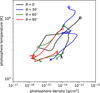 |
Fig. 1 Time evolution of the density and temperature at the photosphere in KN ejecta of an exemplary NS merger simulation (model sym-n1-a6 of Just et al. 2023 with an ejecta mass of 0.073 M⊙) at four different polar angles, θ, relative to the rotation axis of the NS binary. Each line starts at t = 0.1 d (indicated by circles) and ends when the radial optical depth drops below unity (indicated by crosses). |
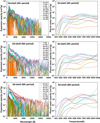 |
Fig. 2 Expansion opacities of the nd group elements for t = 1 day, T = 5000 K, and ρ = 10−13 g cm−3 (left panels) and their corresponding Planck mean opacities (right panels). |
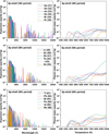 |
Fig. 3 Expansion opacities of the np group elements for t = 1 day, T = 5000 K, and ρ = 10−13 g cm−3 (left panels) and their corresponding Planck mean opacities (right panels). |
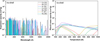 |
Fig. 4 Expansion opacities of the ns group elements for t = 1 day, T = 5000 K, and ρ = 10−13 g cm−3 (left panels) and their corresponding Planck mean opacities (right panels). |
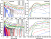 |
Fig. 5 Lanthanide and actinides expansion opacities for t = 1 day, T = 5000 K, and ρ = 10−13 g cm−3 (left panels) and their corresponding Planck mean opacities (right panels). |
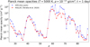 |
Fig. 6 Comparison between Planck mean opacities obtained in this work and the ones from Tanaka et al. (2020) for all elements characterized by Z = 26-88, for t = 1 day post-merger, T = 5000 K, and ρ = 10−13 g cm−3. |
4 Line-binned opacity
In addition to expansion opacities, another frequency-dependent opacity formalism is the so-called line-binned opacity (Fontes et al. 2020):
 (8)
(8)
where ρ is the ejecta density, ∆v are the widths of the frequency bins that contain lines, l, with number densities of the lower level, Nl, and oscillator strengths, fl. This expression is obtained by replacing the line profile with a flat distribution across the corresponding bin (Fontes et al. 2020). Unlike the expansion opacity (Eq. (3)), the line-binned opacity is independent of the evolution time, t, and it can therefore be used for on-the-fly table interpolation in a more straightforward manner.
We thus also computed the line-binned opacities in addition to the expansion ones for lanthanide and actinides species, in order to compare them with other works, as well as their corresponding Planck mean opacities (as defined by Eq. (7)). In particular, we compared our results with the Planck mean line- binned opacities determined by Fontes et al. (2020) and Fontes et al. (2023) for lanthanides (Fig. 7) and actinides (Fig. 8), respectively. The Planck mean line-binned opacities that we computed for all lanthanides and actinides seem to agree to a reasonable extent with the ones from Fontes et al. (2020, 2023), even if our values are systematically slightly higher for lanthanides, with the same conclusion for actinides except for Pa (Z = 91) and Pu (Z = 94). The differences observed are thought to mainly arise from the configurations included in the atomic models.
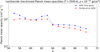 |
Fig. 7 Lanthanide Planck line-binned opacities for T = 3500 K and ρ = 10−13 g cm−3 in comparison with the one computed by Fontes et al. (2020). |
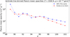 |
Fig. 8 Actinide Planck line-binned opacities for T = 3500 K and ρ = 10−13 g cm−3 in comparison with the one computed by Fontes et al. (2023). |
5 HFR atomic database and opacity tables for kilonovae
In this work, we created a database called “HFR Atomic Database and Opacity Tables for Kilonovae from Mons and Brussels Universities,” which includes, for all the elements considered in this work (i.e., from Z = 20 to Z = 103), all the relevant atomic data to compute expansion and line-binned opacities in the context of KN emissions, as well as expansion and line-binned opacity tables for a grid of typical KN ejecta conditions. The atomic database contains all the energy levels and lines of each element considered in this work computed with the HFR method. As for the expansion and line-binned opacity tables, they are provided for a grid of time post merger, density, and temperature defined as follows: t = 1, 2, 3, 4, 5, 6, 7 days, ρ = 10−17, 10−16, 10−15, 10−14, 10−13 g cm−3, and T = 1000, 2000, 3000, 4000, 5000, 6000, 7000, 8000, 9000, 10 000 K. A table giving the Planck mean opacities of all these elements for the above-mentioned grid of conditions is also supplied. This database is available online on Zenodo1.
6 KN ejecta opacity and light curves
To illustrate the impact of the newly determined HFR opacities, we now consider a state-of-the-art NS merger simulation with the associated post-processed nucleosynthesis calculation, as is described in Just et al. (2023). More specifically, we consider the hydrodynamical simulations of a 1.375-1.375 M⊙ NS merger calculated with the SFHo EoS (Just et al. 2023). The total mass of 2.75 M⊙ corresponds to the estimated total mass of GW170817 event (Abbott et al. 2017a). This end-to-end model, referred to as “sym-n1-a6,” includes the prompt dynamical ejecta component, the ejecta from the NS-torus system formed right after the merger, as well as the subsequently launched ejecta from the black-hole torus before its final evaporation. The masses of the three components amount to 0.006, 0.02, and 0.047 M⊙, respectively, and are sampled by 2380, 375, and 1180 mass elements (also referred to as “trajectories”), respectively. The r-process calculations were performed using the BSkG3 mass model (Grams et al. 2023), the associated TALYS reaction rates obtained with microscopic inputs for the nuclear level densities and photon strength functions (Koning et al. 2023), β-decay rates from the RMF+RRPA model (Marketin et al. 2016), the fission rates based on the HFB-14 model (Goriely et al. 2010), and the fission fragment distributions obtained within the SPY model (Lemaître et al. 2021).
The elemental molar fractions of the 7.3 × 10⁻² M⊙ ejected in this model are shown in Fig. 9 (middle panel) as a function of the atomic number, Z, for the entire ejecta 3.5 days after the NS merger. The contributions of all elements to the Planck mean expansion opacity of the ejecta at t = 3.5 d, T = 6000 K, and ρ = 10−13 g cm−3 are shown in Fig. 9 (lower panel). The partial opacities in this mixture of elements were determined by re-computing the expansion opacity (and, then, Planck mean expansion opacity) of each element by replacing the single-element transition lower level number densities, nl, independent of Z (as is defined in Eq. (4)) by Z-dependent lower level number densities, nl,Z, which were obtained by multiplying the single-element number densities, nl , by the corresponding elemental abundance of each element, yZ ; that is,
 (9)
(9)
For this NS merger model, a major contribution to the total abundance-averaged opacity (for a composition averaged over the entire ejecta) comes from the 3d-shell Z ≃ 24 and 4d-shell Z ≃ 40 elements, in addition to the lanthanides and actinides. The lower opacity of the Z ≃ 24 and Z ≃ 40 elements is compensated by their relatively large abundances. As a consequence, lanthanides do not fully dominate the opacity, at least on average. The ejecta total HFR opacity (equal to 1.13 cm2 g−1) is found to be about 25% lower than the values that would result from the heuristic prescription for the opacities deduced in Just et al. (2022). In that approach, the opacity is parametrically expressed as a function of the lanthanide plus actinide molar fractions (which is equal to 8.4 × 10⁻⁵ in this model) and the gas temperature (see Eqs. (13)–(15) from Just et al. 2022). In addition, it is worth mentioning that estimating the contribution of each element to the ejecta Planck expansion opacity by averaging the single-element Planck opacities (as is shown in Fig. 9; upper panel) with the elemental abundances leads to a rather poor approximation, since a corresponding value of an ejecta total Planck opacity of 0.11 cm2 g−1 would be found in this case; that is, one order of magnitude lower than the actual value. While most works report single-element expansion opacities (i.e., assuming a composition made of 100% of a given element for each species), the latter can therefore not be used to properly estimate the total opacity for a given composition a posteriori, although they are obviously important to compare results between various atomic physics approaches. This is not the case for line-binned opacities, which are directly proportional to the transition lower level number densities (see Eq. (8)), and hence to the elemental abundances.
Similarly, Fig. 10 gives the single-element Planck mean expansion opacities, the molar fractions, and the Planck opacity contributions of all elements just for the rapidly expanding dynamical component of the ejecta in the sym-n1-a6 model. In this case, the ejecta is more abundant in lanthanides and actinides (their molar fraction is equal to 8.7 × 10⁻⁴, i.e., one order of magnitude higher with respect to the entire ejecta case), but also Z ≃ 40 isotopes. The contribution from these three groups of elements is seen to dominate the total abundance- averaged opacity (see Fig. 10, lower panel). In this specific case, at 3.5 days post merger, the phenomenological parametrisation of Just et al. (2022) underestimates the dynamical ejecta opacity by a factor of two, since the HFR total opacity is found to be of 5.42 cm2 g−1, while an opacity of 2.87 cm2 g−1 is obtained when using the formula from Just et al. (2022).
The dependence of the Planck mean opacity of the ejecta with respect to the temperature and density at a time t = 3.5 days post-merger is illustrated in Fig. 11, still considering the overall ejecta composition deduced from NS merger model sym-n1- a6 at t = 3.5 d. It is clear from this figure that the ejecta opacity tends to increase with higher values of density and lower values of temperature, although non-monotonic behavior is also seen, particularly in the temperature dependence, which shows a kind of band structure. At low temperatures, low ionization stages dominate. Since energy levels lie closer to each other in lowly charged ions, higher spectral densities, and thus higher opacities, are expected in this case. This temperature dependence of the ionization structure can therefore explain the opacity increase at decreasing temperatures and the resulting band structure observed in Fig. 11.
The calculated yields and radioactive heating rates were now used as input for a two-dimensional (axisymmetric) radiation transport simulation adopting approximate M1 closure to estimate the KN light curve, as is detailed in Just et al. (2022). The results are shown in Fig. 12. In panel a, a comparison of the bolometric light curves is shown for the parametric opacity function defined in Just et al. (2022) as well as for the case using the opacities calculated by the HFR method described in this paper. For the calculation using the HFR opacities, we adopted the average composition as shown in Fig. 9 and assumed that the ejecta composition is uniformly distributed in the 2D plane. All of the ejecta components are included in this model. Panel b shows the same comparison but assuming that only dynamical ejecta are present, by setting the densities of all other ejecta components to zero and assuming the averaged composition, as is shown in Fig. 10, to be homogeneously distributed in the ejecta. We note that the ejecta composition was not averaged for the simulation with the parametric opacity function. The observed bolometric luminosity of AT2017gfo (Waxman et al. 2018) is also displayed by solid circles for reference. Using the HFR opacities makes a noticeable impact on the light curve compared to the parametric ones. The HFR opacity yields a slightly lower peak bolometric luminosity when all the ejecta components are included, and the time of the peak is shifted toward ~7–8 days, compared to ~1–2 days for the simple parametric opacity approximation of Just et al. (2022). We illustrate in Fig. 13 the time evolution of the averaged photospheric properties and the opacity for the ALCAR-kilonvoa model using the HFR data for the entire ejecta. The photospheric temperature, density, and velocity normalized by their values at 1 day are shown. The Planck mean opacity for both the HFR data and for the parametric opacity function are compared. As is seen in this figure, the opacity is initially higher for the parametric function compared to the HFR opacity until about 1 day, when it drops significantly. The HFR opacity drops more steadily and reaches the minimum value at around ∼7–8 days. This is consistent with the behavior of the model light curves in Fig. 12a. When only the fast dynamical ejecta component is included, the contribution to the opacity is dominated by lanthanides and actinides. In this case, the light curve is comparable for both the opacity calculations, but the peak luminosity is higher for HFR data compared to the parametric opacity approximation. These results illustrate that opacities based on atomic data are sorely needed in order to reliably predict KN light curves.
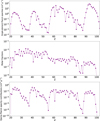 |
Fig. 9 Single-element Planck mean opacities for each species at t = 3.5 d, T = 6000 K, and ρ = 10−13 g cm−3 (upper panel), elemental abundances ejected in the sym-n1-a6 NSM model at t = 3.5 d (Just et al. 2023) (middle panel), and contribution of each element to the Planck mean opacities of the KN ejecta based on the composition resulting in model sym-n1-a6 model 3.5 days post-merger (lower panel). The total Planck opacity of the ejecta (i.e., the HFR Planck mean opacities for this ejecta composition summed over all elements Z) is found to be equal to 1.13 cm2 g−1, whereas an opacity of 1.43 cm2 g−1 is obtained when using the formula from Just et al. (2022). |
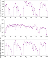 |
Fig. 10 Same as Fig. 9 but only for the dynamical ejecta at t = 3.5 d, T = 2500 K, and ρ = 10−15 g cm−3. In this case, the total HFR opacity is equal to 5.42 cm2 g−1, while the parametric formula from Just et al. (2022) gives an opacity of 2.87 cm2 g−1. |
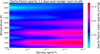 |
Fig. 11 Temperature and density dependence of the Planck mean opacity of the ejecta at a time t = 3.5 days post merger assuming the composition of model sym-n1-a6 at that time. |
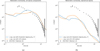 |
Fig. 12 Comparison of light curves obtained with the KN scheme developed in Just et al. (2022) for the NS merger model sym-n1-a6, using a parametric opacity function defined by Just et al. (2022) or the opacity data calculated using the HFR method. The left panel shows the comparison for all the ejecta components including the prompt dynamical component, the ejecta from the NS-torus system, and the disk wind stemming from the black-hole torus remnant; while the right panel shows the comparison for the dynamical ejecta component alone. Note that the computed light curves adopt the simplified assumption of spatially averaged composition. The observed bolometric luminosity of AT2017gfo (Waxman et al. 2018) is shown by solid circles for reference. |
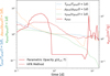 |
Fig. 13 Time evolution of the photospheric properties and the opacity calculated using the HFR method presented in this paper for the NS merger model sym-n1-a6 and assuming a uniform composition corresponding to the full ejecta at t = 3.5 d. Temperature (dotted blue line), density (dotted orange line), and velocity (dotted green line) are scaled by the left y axis and normalized by their values at 1 day. The values at 1 day for these quantities are Tph (t = 1d) = 2750 K, ρph(t = 1d) = 7.4 × 10⁻¹⁶ g cm3, and υph(t = 1d) = 1.2 × 1010 cm s−1, respectively. The Planck-averaged opacity for the HFR data (red, dashed line) is plotted on the right y axis. The solid red curve shows the opacity calculated using the parametric opacity function defined by Just et al. (2022), for comparison. |
7 Conclusions
This work consists of a new large-scale calculation of atomic parameters and opacities for all elements from Ca (Z = 20) to Lr (Z = 103) in their first four charge stages, with a special focus on lanthanides and actinides. This study was carried out in the context of KNe, the electromagnetic counterpart of gravitational wave emission following the coalescence of two NSs, a relevant site of heavy-element production by the r-process. The purpose of this work is to build a database providing more accurate values for the KN ejecta opacity based on detailed atomic calculations. These opacities are of great importance for modeling KN light curves and spectra.
Atomic computations have been performed using the HFR method, which has already been used in our group, in the same context, for Ce II–IV (Carvajal Gallego et al. 2021), for Nd II–III and U II–III (Flörs et al. 2023; Deprince et al. 2023), for Er III (Deprince et al. 2024), for several lighter trans-iron elements (Ben Nasr et al. 2023, 2024), and for many moderately charged lanthanide ions (Carvajal Gallego et al. 2022a,b, 2023a,c; Maison et al. 2022). The strategy adopted in this work is to build the atomic multiconfiguration models of all elements in the charge stages I–IV (which are the species expected to be present in the KN ejecta). Our approach is justified based on the methodology developed in our previous studies for selected lanthanides and actinides (Flörs et al. 2023; Deprince et al. 2023, 2024) as well as the one used for several lighter trans-irons elements (Ben Nasr et al. 2023, 2024), in which we also compare with available experimental data as well as with results obtained using another computational method (namely, FAC, Gu 2008).
The expansion opacities computed for all elements from Ca to Lr using our HFR atomic data are illustrated in this article for typical conditions expected in the KN ejecta one day after merger (namely, at a fiducial temperature of T = 5000 K and a density of ρ = 10−13 g cm−3). The corresponding Planck mean opacities are estimated for a grid of temperatures ranging from T = 1000 K to T = 10 000 K. For such physical conditions within the ejecta, we confirm that lanthanide and actinide opacities are significantly higher than the other trans-iron element ones, which can be explained by the complex atomic structures of these ions characterized by an unfilled 4f and 5f subshell, respectively. Among lanthanides, we note that Sm, Nd, and Pr have the largest opacities, while U, Np, and Pu dominate the actinide expansion opacities. A comparison with the Planck mean expansion opacities determined using HULLAC atomic data for elements with 20 ≤ Z ≤ 88 by Tanaka et al. (2020) is also discussed in detail. From the latter, we conclude that the trends from both calculations agree to a good extent, although HFR Planck mean expansion opacities tend to be larger for several ions, especially for lanthanides by up to one order of magnitude. This disagreement can be explained by the differences between both methods, but especially by the differences in the multiconfiguration models used in both computations. Indeed, Tanaka et al. (2020) use more restricted atomic models as well as approximated atomic partition functions (see Carvajal Gallego et al. 2023b; Banerjee et al. 2024, for more details). In addition, we find that the Planck mean line-binned opacities determined in this work for both lanthanides and actinides are in reasonable agreement with those obtained by Fontes et al. (2020, 2023) (though most of our HFR line-binned opacities are found to be systematically slightly higher).
It is also worth highlighting that we published a database called “HFR Atomic Database and Opacity Tables for Kilonovae from Mons and Brussels Universities”. The latter includes all the relevant data to compute expansion and line-binned opacities in the context of KN emissions, as well as expansion and line- binned opacity tables for a grid of typical KN ejecta conditions.
Finally, we applied our HFR Planck mean expansion opacities to calculate KN light curves using the ALCAR-kilonova code developed in Just et al. (2022) for a 1.375002D-1.375 M⊙ NS merger model (Just et al. 2023). We found that the phenomenological ejecta opacity used by Just et al. (2022) can be significantly different from the one determined using the present HFR atomic data. In addition to lanthanides and actinides, a non- negligible contribution to the opacity comes from the abundant elements around Z ≃ 24 and 40. Lanthanides thus seem to not fully dominate the ejecta opacity, at least on average. The HFR opacities yield a lower luminosity for the first week and shift the peak luminosity to a later day (around 7–8 days) when compared to the phenomenological prescription of Just et al. (2022) (which peaks around ∼2 days). When considering the fast dynamical ejecta only, which are dominated by the abundant f-shell lanthanides and actinides, the phenomenological formula from Just et al. (2022) gives a rather similar light curve for the first 10 days, but the HFR opacities yield a brighter peak. The added value of the phenomenological prescription is that the spatial and temporal dependence of the composition can be taken into account in the calculation of the opacity, something that cannot be easily done with microscopic composition-dependent expansion opacities at the moment. Obviously, opacities based on detailed atomic data are sorely needed to reliably predict light curves. In the present simulations, a uniform composition of the ejecta in the 2D plane has been assumed due to the complex dependence of the expansion opacity on the number densities. An important future improvement in the estimate of KN light curves would consist of calculating the opacities along the ejecta trajectories according to the specific composition of each cell of the 2D grid. Since this calculation represents a significant computer effort, we leave it to future work.
In view of the present results, it would also be worth further improving the HFR atomic data for the species that are found to contribute the most to the KN ejecta opacity, among which feature several lanthanides and actinides (in particular Sm, Nd, Dy, Er, U, Np, and Pu) as well as some lighter trans-iron elements around Z ≃ 24 and Z ≃ 40 (such as Cr, Fe, Zr, and Mo). For these elements, more elaborate atomic models could be tested, for example by enlarging the configuration lists, or by including the so-far neglected core-polarization correction. Fits to experimental energy levels, when available, could also be attempted in a second step to assess the accuracy of our data. An extended stheory-observation comparison of atomic energy levels and line intensities (see e.g., Ding et al. 2024 for Nd III) might indeed allow some semi-empirical adjustment of our computed HFR atomic parameters, and hence improve the resulting opacities.
Data availability
The complete atomic and opacity data sets used in this paper are available on the Zenodo database at the address https://zenodo.org/records/14017952 (DOI 10.5281/zenodo.14017952).
Acknowledgements
The present work is supported by the FWO and F.R.S.- FNRS under the Excellence of Science (EOS) programme (numbers O.0004.22 and O022818F). HCG is a holder of a FRIA fellowship. SG and PP are Research Associate of the Belgian Fund for Scientific Research F.R.S.-FNRS. PQ is F.R.S.-FNRS Research Director. GW, MG, SG and SVE are members of BLU-ULB (Brussels Laboratory of the Universe, blu.ulb.be). OJ acknowledges support by the European Research Council (ERC) under the European Union’s Horizon 2020 research and innovation programme (ERC Advanced Grant KILONOVA No. 885281), by the Deutsche Forschungsgemeinschaft (DFG, German Research Foundation) through Project - ID 279384907 - SFB 1245 (subprojects B06, B07), and by the State of Hesse within the Cluster Project ELEMENTS. Computational resources have been provided by the Consortium des Equipements de Calcul Intensif (CECI), funded by the F.R.S.-FNRS under Grant No. 2.5020.11 and by the Walloon Region of Belgium. We also want to thank our collaborators from GSI, Universidade de Lisboa and NOVA University of Lisbon for fruitful discussions, in particular A. Flörs, R. Silva, J. Marques, G. Martínez-Pinedo and J. Sampaio.
Appendix A configuration lists
List of the configurations used to model each atomic system
References
- Abbott, B., Abbott, R., Abbott, T., et al. 2017a, Phys. Rev. Lett., 119, 161101 [CrossRef] [Google Scholar]
- Abbott, B., Abbott, R., Abbott, T., et al. 2017b, Astrophys. J. Lett., 848, L12 [CrossRef] [Google Scholar]
- Arnould, M., & Goriely, S. 2020, Prog. Part. Nucl. Phys., 112, 103766 [NASA ADS] [CrossRef] [Google Scholar]
- Arnould, M., Goriely, S., & Takahashi, K. 2007, Phys. Repts., 450, 97 [NASA ADS] [CrossRef] [Google Scholar]
- Banerjee, S., Tanaka, M., Kato, D., et al. 2022, ApJ, 934 [Google Scholar]
- Banerjee, S., Tanaka, M., Kato, D., & Gaigalas, G. 2024, ApJ, 968, 64 [NASA ADS] [CrossRef] [Google Scholar]
- Bar-Shalom, A., Klapisch, M., & Oreg, J. 2001, JQSRT, 71, 169 [NASA ADS] [CrossRef] [Google Scholar]
- Ben Nasr, S., Carvajal Gallego, H., Deprince, J., Palmeri, P., & Quinet, P. 2023, A&A, 678, A67 [NASA ADS] [CrossRef] [EDP Sciences] [Google Scholar]
- Ben Nasr, S., Carvajal Gallego, H., Deprince, J., Palmeri, P., & Quinet, P. 2024, A&A, 687, A41 [NASA ADS] [CrossRef] [EDP Sciences] [Google Scholar]
- Blaise, J., & Wyart, J. F. 1992, Energy levels and atomic spectra of actinides (Tables internationales de constantes), 479 [Google Scholar]
- Blaise, J., & Wyart J. F., 1994, http://www.lac.universite-paris-saclay.fr/Data/Database [Google Scholar]
- Carvajal Gallego, H., Palmeri, P., & Quinet, P. 2021, MNRAS, 501, 1440 [Google Scholar]
- Carvajal Gallego, H., Berengut, J., Palmeri, P., & Quinet, P. 2022a, MNRAS, 509, 6138 [Google Scholar]
- Carvajal Gallego, H., Berengut, J., Palmeri, P., & Quinet, P. 2022b, MNRAS, 513, 2302 [NASA ADS] [CrossRef] [Google Scholar]
- Carvajal Gallego, H., Deprince, J., Berengut, J., Palmeri, P., & Quinet, P. 2023a, MNRAS, 518, 332 [Google Scholar]
- Carvajal Gallego, H., Deprince, J., Godefroid, M., et al. 2023b, Eur. Phys. J. D, 77, 72 [NASA ADS] [CrossRef] [Google Scholar]
- Carvajal Gallego, H., Deprince, J., Palmeri, P., & Quinet, P. 2023c, MNRAS, 522, 312 [NASA ADS] [CrossRef] [Google Scholar]
- Cowan, R. D. 1981, The Theory of Atomic Structure and Spectra (University of California Press) [Google Scholar]
- Cowan, J., Sneden, C., Lawler, J., et al. 2021, Rev. Mod. Phys., 93, 015002 [CrossRef] [Google Scholar]
- Deprince, J., Carvajal Gallego, H., Godefroid, M., et al. 2023, Eur. Phys. J. D, 77, 93 [NASA ADS] [CrossRef] [Google Scholar]
- Deprince, J., Carvajal Gallego, H., Ben Nasr, S., et al. 2024, Eur. Phys. J. D, 78, 105 [NASA ADS] [Google Scholar]
- Ding, M., Ryabtsev, A. N., Kononov, E. Y., Ryabchikova, T., & Pickering, J. C. 2024, A&A, 692, A33 [NASA ADS] [CrossRef] [EDP Sciences] [Google Scholar]
- Eastman, R. G., & Pinto, P. A. 1993, ApJ, 412, 731 [NASA ADS] [CrossRef] [Google Scholar]
- Eichler, D., Livio, M., Piran, T., & Schramm, D. 1989, Nature, 340, 126 [NASA ADS] [CrossRef] [Google Scholar]
- Flörs, A., Silva, R. F., Deprince, J., et al. 2023, MNRAS, 524, 3083 [CrossRef] [Google Scholar]
- Fontes, C. J., Fryer, C. L., Hungerford, A. L., Wollaeger, R. T., & Korobkin, O. 2020, MNRAS, 493, 4143 [CrossRef] [Google Scholar]
- Fontes, C. J., Fryer, C. L., Wollaeger, R. T., Mumpower, M. R., & Sprouse, T. M. 2023, MNRAS, 519, 2862 [Google Scholar]
- Gaigalas, G., Kato, D., Rynkun, P., Radžiute, L., & Tanaka, M. 2019, Astrophys. J. Suppl., 240, 29 [NASA ADS] [Google Scholar]
- Gaigalas, G., Rynkun, P., Radžiute, L., et al. 2020, Astrophys. J. Suppl., 248, 13 [NASA ADS] [Google Scholar]
- Gaigalas, G., Rynkun, P., Banerjee, S., et al. 2022, MNRAS, 517, 281 [NASA ADS] [Google Scholar]
- Gillanders, J. H., Smartt, S. J., Sim, S. A., Bauswein, A., & Goriely, S. 2022, Mon. Not. Roy. Astron. Soc., 515, 631 [CrossRef] [Google Scholar]
- Goriely, S., Chamel, N., & Pearson, J. 2010, Phys. Rev. C, 82, 035804 [NASA ADS] [CrossRef] [Google Scholar]
- Goriely, S., Bauswein, A., & Janka, H.-T. 2011, Astrophys. J. Lett., 738, L32 [NASA ADS] [Google Scholar]
- Grams, G., Ryssens, W., Scamps, G., Goriely, S., & Chamel, N. 2023, Eur. Phys. J. A, 59, 270 [Google Scholar]
- Gu, M. F. 2008, Can. J. Phys., 86, 675 [NASA ADS] [CrossRef] [Google Scholar]
- Janka, H.-T. 2017, Handbook of Supernovae, eds. A. W. Alsabti, & P. Murdin (Springer International Pub. AG), 1095 [Google Scholar]
- Just, O., Bauswein, A., Ardevol Pulpillo, R., Goriely, S., & Janka, H.-T. 2015, MNRAS, 448, 541 [Google Scholar]
- Just, O., Goriely, S., Janka, H.-T., Nagataki, S., & Bauswein, A. 2022, MNRAS, 509, 1377 [NASA ADS] [Google Scholar]
- Just, O., Kullmann, I., Goriely, S., et al. 2022, MNRAS, 510, 2820 [NASA ADS] [CrossRef] [Google Scholar]
- Just, O., Vijayan, V., Xiong, Z., et al. 2023, ApJ, 951, L12 [NASA ADS] [CrossRef] [Google Scholar]
- Kasen, D., Badnell, N. R., & Barnes, J. 2013, ApJ, 774, 25 [NASA ADS] [CrossRef] [Google Scholar]
- Kasen, D., Metzger, B., Barnes, J., Quataertl, E., & Ramirez-Ruiz, E. 2017, Nature, 551, 80 [CrossRef] [PubMed] [Google Scholar]
- Koning, A., Hilaire, S., & Goriely, S. 2023, Eur. Phys. J. A, 59, 131 [CrossRef] [Google Scholar]
- Korobkin, O., Rosswog, S., Arcones, A., & Winteler, C. 2012, MNRAS, 26, 1940 [Google Scholar]
- Kullmann, I., Goriely, S., Just, O., Bauswein, A., & Janka, H.-T. 2023, MNRAS, 523, 2551 [NASA ADS] [CrossRef] [Google Scholar]
- Lattimer, J., & Schramm, D. 1974, ApJ, 192, L145 [NASA ADS] [CrossRef] [Google Scholar]
- Lemaître, J.-F., Goriely, S., Bauswein, A., & Janka, H.-T. 2021, Phys. Rev. C, 103, 025806 [CrossRef] [Google Scholar]
- Maison, L., Carvajal Gallego, H., & Quinet, P. 2022, Atoms, 10, 130 [CrossRef] [Google Scholar]
- Marketin, T., Huther, L., & Martinez-Pinedo, G. 2016, Phys. Rev. C, 93, 025805 [CrossRef] [Google Scholar]
- Miller, J. M., Sprouse, T. M., Fryer, C. L., et al. 2019, arXiv e-prints [arXiv:1912.03378] [Google Scholar]
- Peng, Y., Ristic, M., Kedia, A., et al. 2024, Phys. Rev. Res., 6, 033078 [Google Scholar]
- Pognan, Q., Jerkstrand, A., & Grumer, J. 2022, MNRAS, 513, 5174 [NASA ADS] [CrossRef] [Google Scholar]
- Radice, D., Perego, A., Hotokezaka, K., et al. 2018, Astrophys. J, 869, 130 [NASA ADS] [Google Scholar]
- Radžiūtė, L., Gaigalas, G., Kato, D., Rynkun, P., & Tanaka, M. 2020, Astrophys. J. Suppl., 248, 17 [Google Scholar]
- Radžiūtė, L., Gaigalas, G., Kato, D., Rynkun, P., & Tanaka, M. 2021, Astrophys. J. Suppl., 257, 29 [Google Scholar]
- Rosswog, S., Liebendörfer, M., Thielemann, F. K., et al. 1999, A&A, 341, 499 [NASA ADS] [Google Scholar]
- Ruffert, M., Janka, H.-T., & Schaefer, G. 1996, Astron. Astrophys., 311, 532 [NASA ADS] [Google Scholar]
- Rynkun, P., Banerjee, S., Gaigalas, G., et al. 2022, Astron. Astrophys., 658, A82 [NASA ADS] [Google Scholar]
- Siegel, D., Barnes, J., & Metzger, B. 2019, Nature, 569, 241 [CrossRef] [PubMed] [Google Scholar]
- Sobolev, V. V. 1960, Moving Envelopes of Stars (Harvard University Press) [Google Scholar]
- Tanaka, M., & Hotokezaka, K. 2013, ApJ, 775, 113 [NASA ADS] [CrossRef] [Google Scholar]
- Tanaka, M., Kato, D., Gaigalas, G., & Kawaguchi, K. 2020, MNRAS, 496, 1369 [NASA ADS] [CrossRef] [Google Scholar]
- Wanajo, S., Sekiguchi, Y., Nishimura, N., et al. 2014, Astrophys. J. Lett, 789, L39 [NASA ADS] [Google Scholar]
- Wanajo, S., Müller, B., Janka, H.-T., & Heger, A. 2018, Astrophys. J, 853, 40 [NASA ADS] [Google Scholar]
- Wang, T., & Burrows, A. 2023, Astrophys. J, 954, 114 [NASA ADS] [Google Scholar]
- Watson, D., Hansen, C. J., Selsing, J., et al. 2019, Nature, 574, 497 [NASA ADS] [CrossRef] [Google Scholar]
- Waxman, E., Ofek, E. O., Kushnir, D., & Gal-Yam, A. 2018, MNRAS, 481, 3423 [NASA ADS] [CrossRef] [Google Scholar]
- Winteler, C., Käppeli, R., Perego, A., et al. 2012, Astrophys. J, 750, L22 [NASA ADS] [Google Scholar]
- Wyart, J.-F., Blaise, J., Bidelman, W. P., & Cowley, C. R. 1997, Physica Scripta, 56, 446 [Google Scholar]
https://zenodo.org/records/14017952 (DOI 10.5281/zenodo.14017952).
All Tables
All Figures
|
Fig. 1 Time evolution of the density and temperature at the photosphere in KN ejecta of an exemplary NS merger simulation (model sym-n1-a6 of Just et al. 2023 with an ejecta mass of 0.073 M⊙) at four different polar angles, θ, relative to the rotation axis of the NS binary. Each line starts at t = 0.1 d (indicated by circles) and ends when the radial optical depth drops below unity (indicated by crosses). |
| In the text | |
|
Fig. 2 Expansion opacities of the nd group elements for t = 1 day, T = 5000 K, and ρ = 10−13 g cm−3 (left panels) and their corresponding Planck mean opacities (right panels). |
| In the text | |
|
Fig. 3 Expansion opacities of the np group elements for t = 1 day, T = 5000 K, and ρ = 10−13 g cm−3 (left panels) and their corresponding Planck mean opacities (right panels). |
| In the text | |
|
Fig. 4 Expansion opacities of the ns group elements for t = 1 day, T = 5000 K, and ρ = 10−13 g cm−3 (left panels) and their corresponding Planck mean opacities (right panels). |
| In the text | |
|
Fig. 5 Lanthanide and actinides expansion opacities for t = 1 day, T = 5000 K, and ρ = 10−13 g cm−3 (left panels) and their corresponding Planck mean opacities (right panels). |
| In the text | |
|
Fig. 6 Comparison between Planck mean opacities obtained in this work and the ones from Tanaka et al. (2020) for all elements characterized by Z = 26-88, for t = 1 day post-merger, T = 5000 K, and ρ = 10−13 g cm−3. |
| In the text | |
|
Fig. 7 Lanthanide Planck line-binned opacities for T = 3500 K and ρ = 10−13 g cm−3 in comparison with the one computed by Fontes et al. (2020). |
| In the text | |
|
Fig. 8 Actinide Planck line-binned opacities for T = 3500 K and ρ = 10−13 g cm−3 in comparison with the one computed by Fontes et al. (2023). |
| In the text | |
|
Fig. 9 Single-element Planck mean opacities for each species at t = 3.5 d, T = 6000 K, and ρ = 10−13 g cm−3 (upper panel), elemental abundances ejected in the sym-n1-a6 NSM model at t = 3.5 d (Just et al. 2023) (middle panel), and contribution of each element to the Planck mean opacities of the KN ejecta based on the composition resulting in model sym-n1-a6 model 3.5 days post-merger (lower panel). The total Planck opacity of the ejecta (i.e., the HFR Planck mean opacities for this ejecta composition summed over all elements Z) is found to be equal to 1.13 cm2 g−1, whereas an opacity of 1.43 cm2 g−1 is obtained when using the formula from Just et al. (2022). |
| In the text | |
|
Fig. 10 Same as Fig. 9 but only for the dynamical ejecta at t = 3.5 d, T = 2500 K, and ρ = 10−15 g cm−3. In this case, the total HFR opacity is equal to 5.42 cm2 g−1, while the parametric formula from Just et al. (2022) gives an opacity of 2.87 cm2 g−1. |
| In the text | |
|
Fig. 11 Temperature and density dependence of the Planck mean opacity of the ejecta at a time t = 3.5 days post merger assuming the composition of model sym-n1-a6 at that time. |
| In the text | |
|
Fig. 12 Comparison of light curves obtained with the KN scheme developed in Just et al. (2022) for the NS merger model sym-n1-a6, using a parametric opacity function defined by Just et al. (2022) or the opacity data calculated using the HFR method. The left panel shows the comparison for all the ejecta components including the prompt dynamical component, the ejecta from the NS-torus system, and the disk wind stemming from the black-hole torus remnant; while the right panel shows the comparison for the dynamical ejecta component alone. Note that the computed light curves adopt the simplified assumption of spatially averaged composition. The observed bolometric luminosity of AT2017gfo (Waxman et al. 2018) is shown by solid circles for reference. |
| In the text | |
|
Fig. 13 Time evolution of the photospheric properties and the opacity calculated using the HFR method presented in this paper for the NS merger model sym-n1-a6 and assuming a uniform composition corresponding to the full ejecta at t = 3.5 d. Temperature (dotted blue line), density (dotted orange line), and velocity (dotted green line) are scaled by the left y axis and normalized by their values at 1 day. The values at 1 day for these quantities are Tph (t = 1d) = 2750 K, ρph(t = 1d) = 7.4 × 10⁻¹⁶ g cm3, and υph(t = 1d) = 1.2 × 1010 cm s−1, respectively. The Planck-averaged opacity for the HFR data (red, dashed line) is plotted on the right y axis. The solid red curve shows the opacity calculated using the parametric opacity function defined by Just et al. (2022), for comparison. |
| In the text | |
Current usage metrics show cumulative count of Article Views (full-text article views including HTML views, PDF and ePub downloads, according to the available data) and Abstracts Views on Vision4Press platform.
Data correspond to usage on the plateform after 2015. The current usage metrics is available 48-96 hours after online publication and is updated daily on week days.
Initial download of the metrics may take a while.