| Issue |
A&A
Volume 678, October 2023
|
|
|---|---|---|
| Article Number | A67 | |
| Number of page(s) | 11 | |
| Section | Atomic, molecular, and nuclear data | |
| DOI | https://doi.org/10.1051/0004-6361/202346198 | |
| Published online | 05 October 2023 | |
Atomic data and expansion opacity calculations in two representative 4d transition elements, niobium and silver, of interest for kilonovae studies★
1
Physique Atomique et Astrophysique, Université de Mons,
7000
Mons, Belgium
e-mail: This email address is being protected from spambots. You need JavaScript enabled to view it.
; This email address is being protected from spambots. You need JavaScript enabled to view it.
; This email address is being protected from spambots. You need JavaScript enabled to view it.
2
Institut d’Astronomie et d’Astrophysique, Université Libre de Bruxelles,
CP 226,
1050
Brussels, Belgium
3
IPNAS, Université de Liège,
Sart Tilman,
4000
Liège, Belgium
Received:
20
February
2023
Accepted:
23
July
2023
Abstract
Aims. Neutron star (NS) mergers are thought to be a source of heavy trans-iron element production. The latter can be detected in the spectra of the ejected materials, from which bright electromagnetic radiation is emitted. This latter is due to the radioactive decay of the produced heavy r-process nuclei and is known as kilonova. Because of their complex atomic structures – characterized by configurations involving unfilled nd or nf subshells – the heavy elements of the kilonova ejecta often give rise to numerous absorption lines generating significant opacities. The determination of the latter, which are of paramount importance for the analysis of kilonova light curves, requires knowledge of the radiative parameters of the spectral lines belonging to the ions expected to be present in the kilonova ejecta. The aim of the present work is to provide new atomic opacity data for two representative 4d elements, niobium (Nb) and silver (Ag), in their first four charge states, namely for Nb I–IV and Ag I–IV.
Methods. Large-scale calculations based on the pseudo-relativistic Hartree-Fock (HFR) method were performed to obtain the atomic structure and radiative parameters while the expansion formalism was used to estimate the opacities.
Results. Wavelengths and oscillator strengths were computed for several million spectral lines in Nb I–IV and Ag I–IV ions. The reliability of these parameters was estimated by comparison with the few previously published experimental and theoretical results. The newly obtained atomic data were then used to calculate expansion opacities for typical kilonova conditions expected one day after NS merger, a density of ρ = 10−13 g cm−3, and temperatures ranging from T = 5000 K to T =15 000 K.
Key words: atomic data / atomic processes / opacity
Tables 3–10 are available at the CDS via anonymous ftp to cdsarc.cds.unistra.fr (130.79.128.5) or via https://cdsarc.cds.unistra.fr/viz-bin/cat/J/A+A/678/A67
© The Authors 2023
 Open Access article, published by EDP Sciences, under the terms of the Creative Commons Attribution License (https://creativecommons.org/licenses/by/4.0), which permits unrestricted use, distribution, and reproduction in any medium, provided the original work is properly cited.
This article is published in open access under the Subscribe to Open model. This email address is being protected from spambots. You need JavaScript enabled to view it. to support open access publication.
1 Introduction
Material ejected immediately following the collision of two neutron stars (NSs) enriches the Universe with trans-iron heavy elements (Lattimer et al. 1974; Eichler et al. 1989; Freiburghaus et al. 1999; Korobkin et al. 2012; Wanajo et al. 2014). The latter are produced by nucleosynthesis through a rapid neutron capture process, also known as the r-process. The bright electromagnetic emission resulting from the gigantic explosion following the NS merger – referred to as a kilonova – has an electromagnetic spectrum mainly governed by bound-bound opacities and powered by radioactive decay energy of r-process nuclei (see Kasen et al. 2013; Rosswog 2015; Metzger 2017). To determine the kilonova light curve, that is, the evolution of light intensity with time, it is essential to estimate the opacity. Achieving this latter requires a very large amount of radiative data (wavelengths and oscillator strengths), which can be used to characterize the elements present in the ejecta.
Over the last few years, much effort has been made to provide the atomic data necessary for the spectral analysis of kilonovae. Attempts have mainly focused on the lanthanides and actinides, which contribute substantially to kilonova opacities due to their rich spectra, which are charaterized by the unfilled 4f and 5f subshells, respectively. In this context, we must mention the studies carried out for the elements Nd II–IV (Gaigalas et al. 2019), Er III (Gaigalas et al. 2020), Pr-Gd II (Radžiūtė et al. 2020), Tb-Yb II (Radžiūtė et al. 2021), Ce II–IV (Carvajal Gallego et al. 2021), Ce IV (Rynkun et al. 2022), Ce V–X (Carvajal Gallego et al. 2022a), La V–X (Carvajal Gallego et al. 2022b), Pr V–X, Nd V–X, Pm V–X (Carvajal Gallego et al. 2023a), and Sm V–X (Carvajal Gallego et al. 2023b). Atomic data and opacity calculations were also reported by Fontes et al. (2020) and Fontes et al. (2023) for all lanthanide and actinide atoms from neutral (I) to trebly ionized (IV) species, respectively; by Tanaka et al. (2020) for elements ranging from Fe to Ra in the periodic table, in ionization stages from I to IV; and by Banerjee et al. (2022) for three selected lanthanides, namely Nd, Sm, and Eu, from their fourth to their tenth ionization stages (V–XI).
In the present paper, we focus on two representative elements belonging to the fifth row of the periodic table, namely niobium (Nb) and silver (Ag). With their unfilled 4d subshell, the elements of this group make the greatest contribution to opacities after the lanthanides and actinides, as stated by Tanaka et al. (2020). However, according to the latter authors, Nb and Ag ions contribute very differently to the opacities, with the estimated Planck mean opacities being one and two orders of magnitude higher for Nb than for Ag at temperatures Τ =10 000 K and Τ = 5000 K, respectively. The aim of our work is to verify this statement for a somewhat wider temperature range by performing new atomic data and opacity calculations for Nb I–IV and Ag I–IV ions. To do this, we used the pseudo-relativistic Hartree-Fock (HFR) method of Cowan (1981) to obtain the energy levels, wavelengths, transition probabilities, and oscillator strengths for a large number of spectral lines in these ions and estimated the corresponding opacities using the expansion formalism for kilonova ejecta conditions expected one day after the NS merger, namely a density of 10−13 g cm−3 and a temperature ranging from 5000 to 15 000 K.
2 Atomic data calculations
The theoretical method used for computing the atomic structures and the radiative parameters in Nb I–IV and Ag I–IV ions is the pseudo-relativistic Hartree-Fock (HFR) approach originally introduced by Cowan (1981). In order to maintain a similar quality for all calculated atomic states, which is an important factor in the estimation of opacities, no semi-empirical fitting was performed, although some experimental levels are available for the considered ions. To compensate for this, the ab initio values of all the Slater electrostatic integrals (Fk, Gk and Rk) were multiplied by a factor of 0.85, as suggested by Cowan (1981), in order to roughly account for interactions with highly excited configurations not explicitly included in the HFR models. In Tables 1 and 2, we list the multiconfiguration expansions considered in the calculations. An immediate observation that can be made when looking at these tables is that the physical models used in our work are much more elaborate than those considered for the atomic and opacity calculations of Tanaka et al. (2020), giving rise to a total number of levels equal to 21 105 (Nb I), 9278 (Nb II), 2639 (Nb III), 367 (Nb IV), 2147 (Ag I), 8179 (Ag II), 18 189 (Ag III), and 8757 (Ag IV) in our calculations, to be compared with 649, 487, 188, 52, 18, 150, 210, and 507, respectively, in the calculations of Tanaka et al. (2020).
Tables 3–10 list the wavelengths and oscillator strengths obtained with the HFR method for the experimentally observed lines in Nb I–IV and Ag I–IV ions. Only transitions whose cancellation factor (CF) was greater than 0.02 in our calculations are reported in these tables; the computed line strengths characterized by lower CF-values, corresponding for the most part to very weak transitions, must be taken with care because of their greater uncertainties, as described by Cowan (1981).
The accuracy of the HFR results was evaluated through comparisons with available experimental and theoretical data. In the latter, we observed a good overall agreement (within a few percent) between our calculated wavelengths and the published experimental values, also given in Tables 3–10. It was indeed found that the average relative deviations Δλ/λΕxp (with Δλ = λHFR – λΕxp) were equal to 0.0576 ± 0.0028 for Nb I, 0.0319 ± 0.0489 for Nb II, 0.0229 ± 0.0105 for Nb III, 0.0041 ± 0.0081 for Nb IV, 0.0253 ± 0.0573 for Ag I, 0.0200 ± 0.0280 for Ag II, 0.0162 ± 0.0131 for Ag III, and 0.0143 ± 0.0273 for Ag IV when considering the experimental wavelengths reported by Gao et al. (2019; Nb I), Nilsson et al. (Nilsson et al.; Nb II, Nb III), Kramida et al. (Kramida et al.; Nb IV), Pickering & Zilio (2001; Ag I), Kramida et al. (2023; Ag II), Ankita & Tauheed (2018; Ag III), and Ankita & Tauheed (2020; Ag IV). These comparisons are shown in Figs. 1 and 2 for Nb and Ag ions, respectively.
If a good estimate of wavelengths is important for calculating opacities, so too are energy levels, as these are used in the Boltzmann and Saha distributions assumed in the formalism described in the following section. In order to gain an overview of the quality of the energy levels calculated in our work, we plotted the distributions of relative deviations from experimental level energies in Figs. 3 and 4 for Nb and Ag ions, respectively. More precisely, these figures show the number of levels, N, as a function of ΔE/E = EHFR – EExp/EExp. As can be seen, good overall agreement was found when comparing theoretical and experimental levels, the mean deviation ΔE/E being equal to −0.0449 ± 0.1174 for Nb I, −0.0138 ± 0.0596 for Nb II, 0.0045 ± 0.0256 for Nb III, 0.0124 ± 0.0246 for Nb IV, −0.0706 ± 0.0347 for Ag I, −0.0193 ± 0.0266 for Ag II, −0.0125 ± 0.0073 for Ag III, and 0.0115 ± 0.0106 for Ag IV when considering the experimental levels compiled in the NIST database (Kramida et al. 2023) for Nb I–IV, Ag I–III and from Ankita & Tauheed (2020) for Ag IV. In other words, no systematic deviation was observed between HFR and experimental levels for the ions considered, although a greater dispersion must be noted in the case of Nb I.
As regards the oscillator strengths, the results obtained in our work for Nb I–IV and Ag I–IV transitions are compared with previously published data in Tables 3–10. These comparisons are illustrated for each of the ions considered in Figs. 5 and 6, in the case of niobium and silver, respectively. Looking at the details, we notice that our oscillator strengths are generally in good agreement with the data available in the literature. More precisely, for Nb ions, the mean deviations between our gf-values and previous results were found to be of the order of 12% in Nb I when considering the data of Gao et al. (2019); 39% and 19% in Nb II when considering the data of Nilsson et al. (2010) and Ruczkowski et al. (2015), respectively; 15% in Nb III when considering the data of Nilsson et al. (2010); and 37% in Nb IV when considering the data taken from the NIST compilation (Kramida et al. 2023), the latter being deduced from the works carried out by Beck & Pan (2004) and Tauheed & Reader (2005). As far as oscillator strengths in Ag ions are concerned, the mean deviations were found to be 10%, 23%, and 49% in Ag I when comparing with the results reported by Pickering & Zilio (2001), Glowacki & Migdalek (2009), and Kramida et al. (2023), respectively; 85% and 90% in Ag II when considering the data from Ruczkowski et al. (2016) and Kramida et al. (2023), respectively; 10% and 6% in Ag III when considering the results of Zhang et al. (2013) and the gf-values deduced from transition probabilities reported by Ankita & Tauheed (2018); and 30% in Ag IV when comparing our data with the gf’s deduced from the gA-values estimated by Ankita & Tauheed (2020). In summary, we can therefore state that the oscillator strengths calculated in our work for Nb I–IV and Ag I–IV ions are globally within a factor of about two when compared to previously published results. However, it should be noted that most of our HFR radiative parameters were determined from more (or even many more) extensive physical models, that is, containing a larger number of interacting configurations than those used in other theoretical studies. The impact of choosing a sufficiently elaborate physical model on opacity determination, that is, including a sufficient number of well-chosen configurations, was discussed in some of our recent papers (see e.g., Carvajal Gallego et al. 2021, Flörs et al. 2023). In these papers, it was clearly highlighted that the omission of some configurations in the atomic calculations could lead to significant underestimation of the opacity, that is, by up to several orders of magnitude. It was also shown that it is crucial to include all radiative transitions characterized by oscillator strengths down to values as low as 0.00001 in order to achieve convergence in the opacity determination.
It should also be noted that the HFR computational approach is particularly well suited to the determination of opacities, where a similar quality and overall consistency of the radiative parameters for a large number of transitions is by far preferable to a high accuracy of the atomic data for a small set of individual lines. This is mainly due to the orbital optimization procedure implemented by Cowan (1981) in the HFR method. Indeed, in the latter, all the electronic configurations included in the physical model can be assumed to be spectroscopic, because all the average energies are variationally minimized for the whole set of configurations. Each of these configurations is therefore characterized by specifically optimized orbitals, different from those optimized for the other configurations. In contrast, in many other multiconfiguration approaches such as those implemented in the Hebrew University Lawrence Livermore Atomic Code (HULLAC) of Bar-Shalom et al. (2001), in the Flexible Atomic Code (FAC) of Gu (2008), or in the General Relativistic Atomic Structure Package (GRASP) of Grant (2007) and its latest versions, GRASP2K (Jönsson et al. 2013) and GRASP2018 (Froese Fischer et al. 2019), the optimization of the orbitals is generally based on a restricted number of configurations chosen among all the configurations included in the model. Consequently, in these approaches, the calculated atomic parameters might not necessarily be of similar quality for all possible radiative transitions between every configuration, because the latter involve either spectroscopic or correlation orbitals.
Configurations included in the HFR atomic structure calculations for Nb I–IV ions.
Configurations included in the HFR atomic structure calculations for Ag I–IV ions.
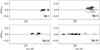 |
Fig. 1 Deviation between HFR and experimental wavelengths, Δλ/λΕxp (Δλ = λHFR – λΕxp) as a function of λHFR for spectral lines in Nb I–IV ions. Experimental data were taken from Gao et al. (2019) for Nb I, from Nilsson et al. (2010) for Nb II and Nb III, and from Kramida et al. (2023) for Nb IV. |
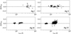 |
Fig. 2 Deviation between HFR and experimental wavelengths, Δλ/λΕxp (Δλ = λHFR – λΕxp) as a function of λHFR for spectral lines in Ag I–IV ions. Experimental data were taken from Pickering & Zilio (2001) for Ag I, from Kramida et al. (2023) for Ag II, from Ankita & Tauheed (2018) for Ag III, and from Ankita & Tauheed (2020) for Ag IV. |
3 Opacity calculations
In a first step, the temperature range within which the Nb I–IV and Ag I–IV ions contribute the most to the plasma ionic abundances was determined from the Saha equation:
 (1)
(1)
where nj and nj−1 are the ionic densities in the j and j − 1 charge stages of the same element, Ue is the electronic partition function (which is defined as 2(mekBT/2πℏ2)3/2), ne is the electron density, χj−1 is the ionization potential of the ion with a j − 1 charge state, kB is the Boltzmann constant, and Uj(T) and Uj−1(T) are the partition functions for charge stages j and j − 1. The latter were computed using all the Nb I–IV and Ag I–IV energy levels obtained in our HFR models described in Sect. 2, completed by Nb V and Ag V energy levels estimated from HFR calculations including configurations of the type 4p6n1,4p54dn1, 4p54f2, 4p55d2, 4p55sn1, 4p44d2nl (n ≤ 8, l ≤ 3), and 4d7, 4d6nl (n ≤ 8, l ≤ 3), 4d54f2,4d55s2,4d55p2,4d55s5p, 4d55s4f, 4d55s5f, 4d55p4f, respectively. The ionization potentials were taken from the NIST database (Kramida et al. 2023).
The ionization balance obtained in this way for the first ions of niobium and silver is shown in Figs. 7 and 8, respectively. By examining these figures, it is clear that the ions considered have maximum relative abundances at T = 2000 K for Nb I and Ag I; T = 4000 K for Nb II; T = 5000 K for Ag II; T = 7500 K for Nb III; T =10 000 K for Ag III; T =13 000 K for Nb IV; and T =15 000 K for Ag IV. We therefore limit ourselves to this temperature range for the opacity calculations in the present work.
To do this, we used the expansion formalism, as described in several publications (see e.g., Karp et al. 1977; Eastman & Pinto 1993; Kasen et al. 2006), according to which the contributions of a large number of lines to the monochromatic opacity are approximated by a discretization involving the summation of lines falling within a spectral width, while the radiative transfer is considered in the Sobolev (1960) approximation. More precisely, in this approach, the bound-bound opacity is calculated by the following expression:
 (2)
(2)
where λ (in Å) is the central wavelength within the region of width Δλ, λl are the wavelengths of the lines appearing in this range, τl are the corresponding optical depths, c (in cm s−1) is the speed of light, ρ (in g cm−3) is the density of the ejected gas, and t (in s) is the elapsed time since the ejection.
The optical depth can be expressed using the Sobolev (1960) expression:
 (3)
(3)
where e (in C) is the elementary charge, me (in g) is the electron mass, fl (dimensionless) is the oscillator strength, and nl (in cm−3) is the density of the lower level of the transition. The latter can be estimated by assuming the local thermodynamic equilibrium (LTE) through the relation
 (4)
(4)
in which gl and El (in cm−1) are the statistical weight and the energy of the lower level of the transition, respectively, U(T) is the partition function of the ionization stage considered, and n is the ion density evaluated by
 (5)
(5)
where A is the mass number, mp is the proton mass, and Xj is the relative ionic fraction of the jth ionization state.
The expansion opacities were computed for Nb I–IV and Ag I–IV ions using all the electric dipole transitions for which the upper level was below the ionization potential and the log gf-value was greater than −5. This led to a very large number of transitions for each element with a total number of 5034 772 lines in Nb I; 1317 786 lines in Nb II; 171 870 lines in Nb III; 11 384 lines in Nb IV; 302 lines in Ag I; 11 869 lines in Ag II; 181423 lines in Ag III; and 963 892 lines in Ag IV. It is important to note that these numbers are much higher than the numbers of transitions included in the opacity calculations of Tanaka et al. (2020) with only 20 961, 27 162, 4452, 336, 60, 642, 5764, and 29 606 lines, respectively. In all our computations, the elapsed time after NS merger was assumed to be t = 1 day and the density of the gas was chosen to be ρ = 10−13 g cm−3, as suggested for example by Banerjee et al. (2022), while the width of the wavelength bins was set to Δλ = 10 Å.
The results obtained are shown in Figs. 9–11, where the calculated opacities of niobium and silver ions are compared for three different temperatures, namely Τ = 5000 K, Τ = 10 000 K, and Τ =15 000 K, respectively. We can clearly see that the contribution of Nb is much more important than that of silver for the first two temperatures, as highlighted by Tanaka et al. (2020) in their Fig. 4, where the Planck mean opacities at Τ = 5000 and 10 000 K are shown for all elements. On the other hand, for the highest temperature considered, Τ =15 000 K, both elements contribute in a similar way to the opacity. This is essentially due to the fact that, at this temperature, the dominant niobium and silver ions are Nb IV and Ag IV, as shown in Figs. 7 and 8 (Nb V, also present at 15 000 K, playing a negligible role in the opacity because of its low number of spectral lines). As the Ag IV ion is characterized by a 4d8 ground configuration, it generates many more transitions of the type 4d8 – 4d7nl, 4d7 nl – 4d7n′l′ and 4d7nl – 4d6nln′l′ than Nb IV whose ground configuration is 4d2. The same observation can also be made for Τ =13 000 K, whose opacities due to Nb and Ag ions are shown in Fig. 12. At this temperature, from Figs. 7 and 8, we can see that the dominant niobium ion is Nb IV, while silver ions are almost equally divided between Ag III and Ag IV, the latter two giving rise to a much higher number of transitions involving the 4dk, 4dk−1nl, and 4dk−2nln′l′ configurations (with k = 9 and 8 for Ag III and IV respectively) than those involving the 4d2, 4dnl, and nln′l′ configurations belonging to Nb IV.
This can be easily understood by estimating the statistical weights of the configurations characterizing the considered ions. Indeed, according to Cowan (1981), for a N-electron configuration expressed in the general form,
 (6)
(6)
with
 (7)
(7)
the total statistical weight is given by
 (8)
(8)
where gi is the statistical weight of the subshell of equivalent electrons  , which can be evaluated as the number of ways we can choose wi different pairs of one-electron quantum numbers mlms from the total of 4li + 2 possible pairs:
 (9)
(9)
Therefore, if we compare the excited configurations 4d4nl for Nb I and 4d10nl for Ag I for example, the statistical weights are given by g(4d4) × g(nl) and g(4d10) × g(nl), respectively, with g(4d4) = 210 and g(4d10) = 1 using the formula (9). This obviously results in a much larger number of energy levels for 4d4nl (Nb I) than for 4d10nl (Ag I). On the other hand, if we carry out the same exercise for the configurations of the type 4dn/ for Nb IV and 4d7nl for Ag IV, we are dealing with statistical weights g(4d) = 10 and g(4d7) = 120, which give rise to many more energy levels within 4d7nl (Ag IV) than within 4dnl (Nb IV).
This is clearly highlighted in Fig. 13 where the distribution of energy levels calculated below the ionization potential is shown for each of the ions considered in our work. Looking at this figure, it is obvious that the density of energy levels decreases from Nb I to Nb IV, while it is the opposite when going from Ag I to Ag IV. In the case of niobium, the number of levels per 1000 cm−1 was indeed found to be equal to 37 (Nb I), 21 (Nb II), 6 (Nb III), and 1 (Nb IV), while for silver this number was equal to 1 (Ag I), 2 (Ag II), 4 (Ag III), and 7 (Ag IV). This higher density of levels – giving a higher density of radiative transitions – for the very first charge states (I, II) of Nb compared to the same charge states of Ag explains the predominance of Nb in the kilonova opacity at the lowest temperatures (T = 5000–10 000 K). On the other hand, as the level densities are similar in the case of Nb III, IV and Ag III, IV ions, the contributions to the opacities of niobium and silver are also similar for kilonova conditions where such ionization degrees are present; that is, for T = 13 000–15 000 K. We note that this behavior is consistent with the trends seen in Fig. 7 reported by Tanaka et al. (2020), where Nb Plank mean opacities decrease with temperature, while Ag opacities increase with temperature.
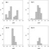 |
Fig. 3 Distribution of energy levels (N) according to the mean deviation ΔE/E = EHFR – EExp/EExp for Nb I–IV. |
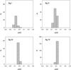 |
Fig. 4 Distribution of energy levels (N) according to the mean deviation ΔE/E = EHFR – EExp/EExp for Ag I–IV. |
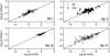 |
Fig. 5 Comparison between HFR oscillator strengths (log gf) and previously published values for Nb I–IV ions. Previous data were taken from Gao et al. (2019) for Nb I, from Nilsson et al. (2010; Nil) and Ruczkowski et al. (2015; Ruc) for Nb II, from Nilsson et al. (2010) for Nb III and from Kramida et al. (2023) for Nb IV. |
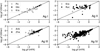 |
Fig. 6 Comparison between HFR oscillator strengths (log gf) and previously published values for Ag I–IV ions. Previous data were taken from Pickering & Zilio (2001; Pic), Glowacki & Migdalek (2009; Glo) and Kramida et al. (2023; Kra) for Ag I, from Ruczkowski et al. (2016; Ruc) and Kramida et al. (2023; Kra) for Ag II, from Zhang et al. (2013; Zha) and Ankita & Tauheed (2018; Ank) for Ag III and from Ankita & Tauheed (2020) for Ag IV. |
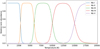 |
Fig. 7 Relative ionic abundances for Nb I–V species as a function of temperature. |
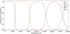 |
Fig. 8 Relative ionic abundances for Ag I–V species as a function of temperature. |
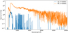 |
Fig. 9 Expansion opacity for Nb and Ag, calculated at Τ = 5000 K. |
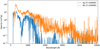 |
Fig. 10 Expansion opacity for Nb and Ag, calculated at Τ =10 000 K. |
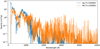 |
Fig. 11 Expansion opacity for Nb and Ag, calculated at Τ = 15 000 K. |
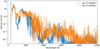 |
Fig. 12 Expansion opacity for Nb and Ag, calculated at T =13 000 K. |
4 Summary and conclusion
Here, we show how we obtained a new consistent set of atomic parameters for radiative transitions belonging to the first ions of two representative 4d elements, namely Nb and Ag. More precisely, energy levels, wavelengths, and oscillator strengths were determined for a large number of spectral lines in Nb I–IV and Ag I–IV ions using the pseudo-relativistic Hartree-Fock (HFR) theoretical approach. For many of these lines, the gf-values were obtained for the first time. From these results, the reliability of which we were able to verify through comparisons with previously published experimental and theoretical data, the expansion opacities were computed for kilonova conditions corresponding to one day after a neutron star merger, a density of 10−13 g cm−3, and a temperature range from 5000 to 15 000 K. This allowed us to highlight that, although the contribution to the opacity is much more important for Nb than for Ag up to T = 10 000 K, both elements contribute similarly at T =15 000 K. This is mainly due to the fact that the configurations characterizing the Nb ions have a decreasing complexity (i.e., with a decreasing number of levels) from Nb I to Nb IV, whereas the opposite is true for the Ag ions, where the configurations have an increasing complexity from Ag I to Ag IV.
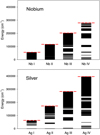 |
Fig. 13 Calculated energy levels below the ionization limit for Nb I–IV and Ag I–IV ions. For each ion, the dashed red line corresponds to the ionization potential taken from the NIST database (Kramida et al. 2023). |
Acknowledgements
H.C.G. is holder of a FRIA fellowship while P.P. and P.Q. are, respectively, Research Associate and Research Director of the Belgian Fund for Scientific Research F.R.S.-FNRS. This project has received funding from the FWO and F.R.S.-FNRS under the Excellence of Science (EOS) programme (Grant Nos. O.0228.18 and O.0004.22). Part of the atomic calculations were made with computational resources provided by the Consortium des Équipements de Calcul Intensif (CECI), funded by the F.R.S.-FNRS under Grant No. 2.5020.11 and by the Walloon Region of Belgium.
References
- Ankita, S., & Tauheed, A. 2018, JQSRT, 05, 022 [Google Scholar]
- Ankita, S., & Tauheed, A. 2020, JQSRT, 254, 107193 [NASA ADS] [CrossRef] [Google Scholar]
- Banerjee, S., Tanaka, M., Kawaguchi, K., Kato, D., & Gaigalas, G. 2020, ApJ, 901, 29 [NASA ADS] [CrossRef] [Google Scholar]
- Banerjee, S., Tanaka, M., Kato, D., Gaigalas, G., Kawaguchi, K., & Domoto, N., 2022, ApJ, 934, 117 [CrossRef] [Google Scholar]
- Bar-Shalom, A., Klapisch, M., & Oreg, J. 2001, JQSRT, 71, 169 [NASA ADS] [CrossRef] [Google Scholar]
- Beck, D. R., & Pan, L. 2004, Phys. Scr., 69, 91 [NASA ADS] [CrossRef] [Google Scholar]
- Carvajal Gallego, H., Palmeri, P., & Quinet P. 2021, MNRAS, 501, 1440 [Google Scholar]
- Carvajal Gallego, H., Berengut, J. C., Palmeri, P., & Quinet, P. 2022a, MNRAS, 509, 6138 [Google Scholar]
- Carvajal Gallego, H., Berengut, J. C., Palmeri, P., & Quinet, P. 2022b, MNRAS, 513, 2302 [NASA ADS] [CrossRef] [Google Scholar]
- Carvajal Gallego, H., Deprince, J., Berengut, J. C., Palmeri, P., & Quinet, P. 2023a, MNRAS, 518, 332 [Google Scholar]
- Carvajal Gallego, H., Deprince, J., Palmeri, P., & Quinet, P. 2023b, MNRAS, submitted [Google Scholar]
- Cowan, R. D. 1981, The Theory of Atomic Structure and Spectra (Berkeley: California University Press) [Google Scholar]
- Eastman, R. G., & Pinto, P. A. 1993, ApJ, 412, 731 [NASA ADS] [CrossRef] [Google Scholar]
- Eichler, D., Livio, M., Piran, T., & Schramm, D. N. 1989, Nature, 340, 126 [NASA ADS] [CrossRef] [Google Scholar]
- Flörs, A., Silva, R. F., Deprince, J., et al. 2023, MNRAS, 524, 3083 [CrossRef] [Google Scholar]
- Fontes, C. J., Fryer, C. L., Hungerford, A. L., Wollaeger, R. T., & Korobkin, O. 2020, MNRAS, 493, 4143 [CrossRef] [Google Scholar]
- Fontes, C. J., Fryer, C. L., Wollaeger, R. T., Mimpower, M. R., & Sprouse, T. M. 2023, MNRAS 519, 2862 [Google Scholar]
- Freiburghaus, C., Rosswog, S., & Thielemann, F. K. 1999, ApJ, 525, L121 [NASA ADS] [CrossRef] [Google Scholar]
- Froese Fischer, C., Gaigalas, G., Jönsson, P., & Bieron, J. 2019, Comput. Phys. Commun., 237, 184 [NASA ADS] [CrossRef] [Google Scholar]
- Gaigalas, G., Kato, D., Rynkun, P., Radžiūtė, L., & Tanaka, M. 2019, ApJS, 240, 29 [NASA ADS] [CrossRef] [Google Scholar]
- Gaigalas, G., Rynkun, P., Radziüte, et al. 2020, ApJS, 248, 13 [CrossRef] [Google Scholar]
- Gao, Y., Geng, Y., Quinet, P., et al. 2019, ApJS, 242, 23 [NASA ADS] [CrossRef] [Google Scholar]
- Glowacki, L., & Migdalek, J. 2009, Phys. Rev. A, 80, 042505 [NASA ADS] [CrossRef] [Google Scholar]
- Grant, I. P. 2007, Relativistic Quantum Theory of Atoms and Molecules (Springer) [CrossRef] [Google Scholar]
- Gu, M. F. 2008, Can. J. Phys., 86, 675 [NASA ADS] [CrossRef] [Google Scholar]
- Jönsson, P., Gaigalas, G., Bieron, J., Froese Fischer, C., & Grant, I. P. 2013, Comput. Phys. Commun., 184, 2197 [CrossRef] [Google Scholar]
- Karp, A. H., Lasher, G., Chan, K. L., & Salpeter, E. E. 1977, ApJ, 214, 161 [NASA ADS] [CrossRef] [Google Scholar]
- Kasen, D., Thomas, R. C., & Nugent, P. 2006, ApJ, 651, 366 [NASA ADS] [CrossRef] [Google Scholar]
- Kasen, D., Badnell, N. R., & Barnes, J. 2013, ApJ, 774, 25 [NASA ADS] [CrossRef] [Google Scholar]
- Korobkin, O., Rosswog, S., Arcones, A., & Winteler, C. 2012, MNRAS, 426, 1940 [NASA ADS] [CrossRef] [Google Scholar]
- Kramida, A., Ralchenko, Yu., Reader, J., & NIST ASD Team 2023, NIST Atomic Database (Gaithersburg, MD: National Institute of Standards and Technology) [Google Scholar]
- Lattimer, J. M., & Schramm, D. N. 1974, ApJ, 192, L145 [NASA ADS] [CrossRef] [Google Scholar]
- Metzger, B. D. 2017, Living Rev. Relativ., 20, 3 [NASA ADS] [CrossRef] [Google Scholar]
- Metzger, B. D., Martínez-Pinedo, G., Darbha, S., et al. 2010, MNRAS, 406, 2650 [NASA ADS] [CrossRef] [Google Scholar]
- Nilsson, H., Hartman, H., Engström, L., et al. 2010, A & A, 511, A16 [NASA ADS] [CrossRef] [EDP Sciences] [Google Scholar]
- Pickering, J. C., & Zilio, V. 2001, Eur. Phys. J. D, 181, 13 [Google Scholar]
- Radžiūtė, L., Gaigalas, G., Kato, D., Rynkun, P., & Tanaka, M. 2020, ApJS, 248, 17 [CrossRef] [Google Scholar]
- Radžiūtė, L., Gaigalas, G., Kato, D., Rynkun, P., & Tanaka, M. 2021, ApJS, 257, 29 [CrossRef] [Google Scholar]
- Rosswog, S. 2015, Int. J. Mod. Phys. D, 24, 1530012 [NASA ADS] [CrossRef] [Google Scholar]
- Ruczkowski, J., Bouazza, S., Elantkowska, M., & Dembczyński, J. 2015, JQSRT, 155, 1 [NASA ADS] [CrossRef] [Google Scholar]
- Ruczkowski, J., Elantkowska, M., & Dembczynski, J. 2016, MNRAS, 459, 3768 [NASA ADS] [CrossRef] [Google Scholar]
- Rynkun, P., Banerjee, S., Gaigalas, G., et al. 2022, A & A, 658, A82 [NASA ADS] [CrossRef] [EDP Sciences] [Google Scholar]
- Sobolev, V. V. 1960, Moving Envelopes of Stars (Cambridge, MA: Harvard University Press) [Google Scholar]
- Tanaka, M., Kato, D., Gaigalas, G., & Kawaguchi, K. 2020, MNRAS, 496, 1369 [NASA ADS] [CrossRef] [Google Scholar]
- Tauheed, A., & Reader, J. 2005, Phys. Scr., 72, 158 [NASA ADS] [CrossRef] [Google Scholar]
- Wanajo, S., Sekiguchi, Y., Nishimura, N., et al. 2014, ApJ, 789, L39 [Google Scholar]
- Zhang, W., Palmeri, P., & Quinet, P. 2013, Phys. Scr., 88, 065302 [NASA ADS] [CrossRef] [Google Scholar]
All Tables
Configurations included in the HFR atomic structure calculations for Nb I–IV ions.
Configurations included in the HFR atomic structure calculations for Ag I–IV ions.
All Figures
|
Fig. 1 Deviation between HFR and experimental wavelengths, Δλ/λΕxp (Δλ = λHFR – λΕxp) as a function of λHFR for spectral lines in Nb I–IV ions. Experimental data were taken from Gao et al. (2019) for Nb I, from Nilsson et al. (2010) for Nb II and Nb III, and from Kramida et al. (2023) for Nb IV. |
| In the text | |
|
Fig. 2 Deviation between HFR and experimental wavelengths, Δλ/λΕxp (Δλ = λHFR – λΕxp) as a function of λHFR for spectral lines in Ag I–IV ions. Experimental data were taken from Pickering & Zilio (2001) for Ag I, from Kramida et al. (2023) for Ag II, from Ankita & Tauheed (2018) for Ag III, and from Ankita & Tauheed (2020) for Ag IV. |
| In the text | |
|
Fig. 3 Distribution of energy levels (N) according to the mean deviation ΔE/E = EHFR – EExp/EExp for Nb I–IV. |
| In the text | |
|
Fig. 4 Distribution of energy levels (N) according to the mean deviation ΔE/E = EHFR – EExp/EExp for Ag I–IV. |
| In the text | |
|
Fig. 5 Comparison between HFR oscillator strengths (log gf) and previously published values for Nb I–IV ions. Previous data were taken from Gao et al. (2019) for Nb I, from Nilsson et al. (2010; Nil) and Ruczkowski et al. (2015; Ruc) for Nb II, from Nilsson et al. (2010) for Nb III and from Kramida et al. (2023) for Nb IV. |
| In the text | |
|
Fig. 6 Comparison between HFR oscillator strengths (log gf) and previously published values for Ag I–IV ions. Previous data were taken from Pickering & Zilio (2001; Pic), Glowacki & Migdalek (2009; Glo) and Kramida et al. (2023; Kra) for Ag I, from Ruczkowski et al. (2016; Ruc) and Kramida et al. (2023; Kra) for Ag II, from Zhang et al. (2013; Zha) and Ankita & Tauheed (2018; Ank) for Ag III and from Ankita & Tauheed (2020) for Ag IV. |
| In the text | |
|
Fig. 7 Relative ionic abundances for Nb I–V species as a function of temperature. |
| In the text | |
|
Fig. 8 Relative ionic abundances for Ag I–V species as a function of temperature. |
| In the text | |
|
Fig. 9 Expansion opacity for Nb and Ag, calculated at Τ = 5000 K. |
| In the text | |
|
Fig. 10 Expansion opacity for Nb and Ag, calculated at Τ =10 000 K. |
| In the text | |
|
Fig. 11 Expansion opacity for Nb and Ag, calculated at Τ = 15 000 K. |
| In the text | |
|
Fig. 12 Expansion opacity for Nb and Ag, calculated at T =13 000 K. |
| In the text | |
|
Fig. 13 Calculated energy levels below the ionization limit for Nb I–IV and Ag I–IV ions. For each ion, the dashed red line corresponds to the ionization potential taken from the NIST database (Kramida et al. 2023). |
| In the text | |
Current usage metrics show cumulative count of Article Views (full-text article views including HTML views, PDF and ePub downloads, according to the available data) and Abstracts Views on Vision4Press platform.
Data correspond to usage on the plateform after 2015. The current usage metrics is available 48-96 hours after online publication and is updated daily on week days.
Initial download of the metrics may take a while.