| Issue |
A&A
Volume 687, July 2024
|
|
|---|---|---|
| Article Number | A41 | |
| Number of page(s) | 15 | |
| Section | Atomic, molecular, and nuclear data | |
| DOI | https://doi.org/10.1051/0004-6361/202348919 | |
| Published online | 25 June 2024 | |
Comparative study of kilonova opacities for three elements of the sixth period (hafnium, osmium, and gold) from new atomic structure calculations in Hf I–IV, Os I–IV, and Au I–IV★
1
Physique Atomique et Astrophysique, Université de Mons,
7000
Mons,
Belgium
e-mail: This email address is being protected from spambots. You need JavaScript enabled to view it.
; This email address is being protected from spambots. You need JavaScript enabled to view it.
; This email address is being protected from spambots. You need JavaScript enabled to view it.
2
Institut d’Astronomie et d’Astrophysique, Université Libre de Bruxelles,
CP 226,
1050
Brussels,
Belgium
3
IPNAS, Université de Liège, Sart Tilman,
4000
Liège,
Belgium
Received:
12
December
2023
Accepted:
15
February
2024
Abstract
Aims. It is now well established that a large amount of heavy (trans-iron) elements are produced during neutron star (NS) mergers. These elements can be detected in the spectra of the kilonova emitted from the post-merger ejected materials. Due to the high level densities that characterize the complex configurations belonging to heavy elements, thus giving rise to millions of absorption lines, the kilonova ejecta opacity is of significant importance. The elements that contribute the most to the latter are those with an unfilled nd subshell belonging to the fifth and the sixth rows of the periodic table, and those with an unfilled nf subshell belonging to the lanthanide and actinide groups. The aim of the present work is to make a new contribution to this field by performing large-scale atomic structure calculations in three specific sixth-row 5d elements, namely hafnium, osmium, and gold, in the first four charge stages (I–IV), and by computing the corresponding opacities, while focusing on the importance of the atomic models used.
Methods. The pseudo-relativistic Hartree–Fock (HFR) method, including extended sets of interacting configurations, was used for the atomic structure and radiative parameter calculations, while the expansion formalism was used to estimate the opacities.
Results. Theoretical energy levels, wavelengths, and oscillator strengths were computed for millions of spectral lines in Hf I–IV, Os I–IV, and Au I–IV ions, the reliability of these parameters being assessed through detailed comparisons with previously published experimental and theoretical results. The newly obtained atomic data were then used to calculate expansion opacities for typical kilonova conditions expected one day after the NS merger; these are a density of ρ = 10−13 g cm−3 and temperatures ranging from T = 5000 K to T = 15 000 K. Some agreements and differences were found when comparing our results with available data, highlighting the importance of using sufficiently complete atomic models for the determination of opacities.
Key words: atomic data / atomic processes / opacity
Tables 2–13 are available at the CDS via anonymous ftp to cdsarc.cds.unistra.fr (130.79.128.5) or via https://cdsarc.cds.unistra.fr/viz-bin/cat/J/A+A/687/A41
© The Authors 2024
 Open Access article, published by EDP Sciences, under the terms of the Creative Commons Attribution License (https://creativecommons.org/licenses/by/4.0), which permits unrestricted use, distribution, and reproduction in any medium, provided the original work is properly cited.
This article is published in open access under the Subscribe to Open model. This email address is being protected from spambots. You need JavaScript enabled to view it. to support open access publication.
1 Introduction
A kilonova, which is the electromagnetic signal that happens when two neutron stars (NS) merge, is known to be the place where heavy (trans-iron) chemical elements show large contributions to the spectrum (Lattimer et al. 1974; Eichler et al. 1989; Freiburghaus et al. 1999; Korobkin et al. 2012; Wanajo et al. 2014; Kasen et al. 2013, 2017; Rosswog 2015; Metzger 2017). These elements are produced from the rapid nucleosynthesis r-process during the NS coalescence, and, because of their high density of electronic transitions between numerous energy levels, the emitted light is strongly absorbed, leading to a significant opacity characterizing the kilonova spectra.
While many approaches of kilonova spectral modeling assume constant gray opacities (Perego et al. 2017; Villar et al. 2017) or use opacities determined from prescriptions consisting of crude approximations to atomic-physics-based models (Just et al. 2022), the accurate estimation of this opacity is of paramount importance for kilonova light-curve determination, that is, the evolution of kilonova luminosity with time (Kasen et al. 2013; Tanaka et al. 2020). This relies on the most comprehensive knowledge possible of atomic data such as energy levels, wavelengths, and oscillator strengths characterizing the species contributing most to the opacity. Among the latter, we essentially find the elements with an open 4d or 5d subshell belonging to the fifth and sixth rows of the periodic table and the elements with an open 4f or 5f subshell belonging to the lanthanide and actinide groups (Tanaka et al. 2020).
In this context, many recent works have been dedicated to new extended calculations of atomic parameters in heavy elements with the aim of deducing the corresponding opacities. Most of these studies were focused on lanthanide ions, such as the papers published by Gaigalas et al. (2019) for Nd II–IV, Gaigalas et al. (2020) for Er III, Radžiūtė et al. (2020) for Pr II–Gd II, Radžiūtė et al. (2021) for Tb II–Yb II, Carvajal Gallego et al. (2021) for Ce II–IV, Rynkun et al. (2022) for Ce IV, Carvajal Gallego et al. (2022a) for Ce V–X, Carvajal Gallego et al. (2022b) for La V–X, Carvajal Gallego et al. (2023a) for Pr V–X, Nd V–X, Pm V–X, Carvajal Gallego et al. (2023b) for Sm V–X, and Maison et al. (2022) for Lu V.
Atomic structure and opacity calculations were also investigated by Fontes et al. (2020, 2023) for all lanthanide and actinide atoms in charge stages between I and IV, by Tanaka et al. (2020) for elements ranging from Fe to Ra in ionization stages from I to IV, by Banerjee et al. (2022) for three selected lanthanides (i.e., Nd, Sm and Eu, from V to XI), and by Banerjee et al. (2024) for all elements from La to Ra in the charge stages ranging from I to XI. We also highlight the recent studies concerning kilonova opacities relating to neodymium and uranium ions using different atomic structure approaches (Flörs et al. 2023) as well as analyses of the sensitivity of astrophysical opacities to atomic data in relation to the use of a semiempirical adjustment of radial parameters, the introduction of core-polarization effects (Deprince et al. 2023), or the use of complete partition functions (Carvajal Gallego et al. 2023c) in the calculations.
In the present work, we report the results of a comparative study of the contributions to kilonova expansion and Planck mean opacities for three representative 5d-elements of the sixth period, namely hafnium, osmium, and gold, for which extended configuration interaction models based on the pseudo-relativistic Hartree–Fock (HFR) method were used to obtain a new set of radiative data for a large amount of lines belonging to the first four spectra (i.e., Hf I–IV, Os I–IV, and Au I–IV). These data were then considered for the determination of the corresponding expansion and Planck mean opacities for kilonova ejecta conditions expected one day after the NS merger, that is, for a density of 10−13 g cm−3 and a temperature ranging from 5000 to 15 000 K. This work follows a similar study that we recently published for two representative 4d-transition elements of the fifth period, namely niobium and silver (Ben Nasr et al. 2023).
2 Atomic data
Theoretical energy levels, wavelengths, and oscillator strengths for spectral lines in Hf I–IV, Os I–IV, and Au I–IV were computed using the pseudo-relativistic Hartree–Fock (HFR) approach developed by Cowan (1981). For each atomic system, a large amount of interacting configurations were included in the calculations. The complete lists of these multi-configuration expansions are given in Tables A.1–A.3 for Hf, Os, and Au ions, respectively. No semi-empirical procedure, in which configuration average energies would have been fit to match available experimental data, was performed. It was indeed showed by Deprince et al. (2023) that computed opacities are virtually not affected by such an adjustment. However, all the Slater radial integrals, corresponding to the direct (Fk) and the exchange (Gk) electrostatic interactions between electrons within the same configurations and to the electrostatic interactions between electrons belonging to different configurations (Rk) were scaled down by a factor of 0.85, while the spin-orbit parameters (ζnl) were kept at their ab initio values, as recommended by Cowan (1981). It was actually shown by the latter that this procedure made it possible to reduce the differences between the HFR energy levels and the experimental values, when they are available. Nevertheless, it is useful to remember that the choice of this scaling factor (between for example 0.80, 0.85, 0.90, and 0.95) does not have a critical impact on the opacity calculations, as discussed in one of our previous papers (Carvajal Gallego et al. 2023a).
The improvement in agreement between theoretical and experimental levels when the scaling factor (S F) is used in HFR calculations is illustrated in Tables A.4–A.6, where we give a small sample comparison between the first few experimentally known energy levels and the HFR values obtained without scaling down the Slater integrals and with the scaling factor 0.85 for Hf I–IV, Os I–IV, and Au I–IV ions, respectively. If the improvement is not always obvious for some specific levels, we note that the overall agreement is better when applying the scaling factor, the mean deviation ΔE = EHFR − EExp being found to be equal to 563 cm−1 for all the levels reported in Tables A.4–A.6, while the same deviation is a factor of two larger (ΔE = 1154 cm−1) when no scaling factor is applied to the Slater integrals. Of course, the agreement between calculated and experimental levels can always be improved by a semi-empirical adjustment procedure, as suggested by Cowan (1981), but it has been shown (Deprince et al. 2023) that such a procedure has no significant impact on the determination of opacities in the most interesting spectral region for current observations, typically beyond 3000 Å.
Using the physical models considered in our HFR calculations, a large number of spectroscopic parameters were obtained. More precisely, the configurations listed in Tables A.1–A.3 gave rise to numerous energy levels and radiative transitions whose numbers are reported in Table 1. We note that the numbers of transitions given in this table correspond to those involving energy levels below the ionization potential of each atom or ion (whose value taken from the NIST database (Kramida et al. 2023) is also given in Table 1) and for which the computed log gf-values were found to be greater than −5. This lower limit on the oscillator strengths was actually shown to allow the inclusion of the large majority of transitions contributing to the opacity in one of our previous papers (Carvajal Gallego et al. 2021).
To have an idea of the extent of the atomic structure calculations carried out in the present work, we compare the number of levels that we obtained with those resulting from the theoretical models considered by Tanaka et al. (2020) for the same ions in Fig. 1. More precisely, in this figure we plot the full set of energy levels calculated in the present work along with those obtained using the HFR method only including the configurations listed in Tanaka et al. (2020) for Hf I–IV, Os I–IV, and Au I–IV. We can easily see that, for some ions, the level densities are considerably larger in our calculations than what was deduced from the models of Tanaka et al., which may turn out to be an essential criterion for the determination of opacities. More precisely, we note rather large differences between both sets of energy levels in the cases of Hf III and Hf IV, in particular as far as highly excited states are concerned. Such differences are also observed, to a lesser extent, for states just below the ionization potential in the cases of Hf II, Os IV, Au II, and Au IV. Unfortunately, for most ions, there are so many levels that it is difficult to distinguish the differences between the level densities obtained in both works in Fig. 1. To highlight such differences, an example is given in Fig. 2 in which we have enlarged part of Fig. 1 corresponding to the Os II energy levels between 120000 and 138 000 cm−1, clearly showing that the level density obtained in our calculations is much higher than the one deduced from Tanaka et al. (2020).
The reliability of our results was assessed through detailed comparisons with other previously published experimental and theoretical data. In particular, the HFR wavelengths obtained in the present work were found to be in good agreement (within a few percent) with the available experimental values. Indeed, the average relative deviations Δλ/λExp (with Δλ = λHFR − λExp) were evaluated at 0.002 ± 0.060 for Hf I, 0.028 ± 0.068 for Hf II, 0.030 ± 0.073 for Hf III, 0.031 ± 0.036 for Hf IV, 0.053 ± 0.179 for Os I, 0.007 ± 0.079 for Os II, 0.011 ± 0.030 for Os III, 0.004 ± 0.020 for Os IV, 0.025 ± 0.081 for Au I, 0.017 ± 0.042 for Au II, 0.018 ± 0.042 for Au III, and 0.023 ± 0.010 for Au IV when taking the experimental wavelengths from Kramida et al. (2023) for Hf I–II, Os III, and Au I, from Malcheva et al. (2009) for Hf III, from Sugar et al. (1974) for Hf IV, from Ivarsson et al. (2003) and Quinet et al. (2006) for Os I, from Ivarsson et al. (2004) and Quinet et al. (2006) for Os II, from Ryabtsev et al. (1998) for Os IV, from Ryabtsev et al. (1998) for Au II, from Zainab & Tauheed (2019) for Au III, and from Wyart et al. (1994) for Au IV. These relative deviations Δλ/λExp are plotted as a function of λHFR in Fig. 3 for neutral, single-, double-, and treble-ionized hafnium, osmium, and gold.
An estimate of the quality of our oscillator strengths could also be made from comparisons with previously published data. However, as the primary goal of our work was to determine opacities, it was more useful to ensure the overall consistency of our calculated gf-values for the whole set of transitions in the ions of interest than to examine their accuracy for each individual transition in detail. For this purpose, in Figs. 4–6 we show the comparisons of the log gf-values obtained in the present work with the experimental and theoretical results taken from literature for Hf I–III, Os I–IV, and Au I–IV, respectively. As can be seen in these figures, the overall agreement is satisfactory, the deviation being found to be less than a factor of two for 84% of transitions in Hf I–III, for 70% of transitions in Os I–IV, and for 77% of transitions in Au I–IV, when considering the data from Duquette et al. (1986) for Hf I; Lundqvist et al. (2006), Lawler et al. (2007), Bouazza et al. (2015), and Den Hartog et al. (2021) for Hf II; Malcheva et al. (2009) for Hf III; Kurucz (1993), Ivarsson et al. (2003), and Quinet et al. (2006) for Os I; Ivarsson et al. (2004) and Quinet et al. (2006) for Os II; Azarov et al. (2018) for Os III; Ryabtsev et al. (1998) for Os IV; Corliss et al. (1981), Migdalek & Baylis (1979), Hannaford et al. (1981), Desclaux et al. (1994), Gaarde et al. (1994), Migdalek & Garmulewicz (2000), Safronova & Johnson (2004), Fivet et al. (2007), Zhang et al. (2018), McCann et al. (2022), and Kramida et al. (2023) for Au I; Zhang et al. (2002), Biémont et al. (2007), and McCann et al. (2022) for Au II; Enzonga et al. (2008) and Zainab & Tauheed (2019) for Au III; and Wyart et al. (1994) for Au IV. It is also worth emphasizing that no systematic deviation was observed between our oscillator strengths and the other results.
All these comparisons allowed us to have some confidence in the overall reliability of the radiative parameters obtained in the present work, the main purpose of which is to to provide a large quantity of atomic data of sufficient quality for the estimation of opacities. For more numerical details, some samples of our newly calculated oscillator strengths (log gf) are compared with previously published results for experimentally observed intense lines in Hf I–IV, Os I–IV, and Au I–IV in Tables 2–13 (only available at the CDS). It should be noted that, in these tables, among the tens of millions of lines computed in our work, we restricted ourselves to the strongest transitions for which the oscillator strengths did not present significant cancellation effects in the HFR calculations, i.e. for which the cancellation factor, CF as defined by Cowan (1981) was greater than 0.05, and to transitions providing points of comparison with experimental or theoretical results previously published in the literature. Looking at these tables, one can obviously notice that, although the overall agreement is satisfactory (on the order of a factor of two), some of our oscillator strengths can present relatively large disagreements with results previously published in the literature. This is mainly due to the fact that our atomic calculations were not optimized for particular transitions but rather aimed at providing a set of spectroscopic parameters of sufficient and similar quality for a very large number (several hundred thousand) of radiative transitions, which constitutes an essential point for opacity calculations.
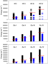 |
Fig. 1 Comparison between full set of HFR energy levels calculated using the physical models of the present work (in black) and the HFR energy levels obtained using the physical models considered by Tanaka et al. (2020) (in blue) for Hf I–IV, Os I–IV, and Au I–IV. The red lines correspond to the ionization potentials taken from the NIST database (Kramida et al. 2023). |
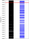 |
Fig. 2 Comparison between full set of HFR energy levels calculated using physical models of present work (in black) and HFR energy levels obtained using physical models considered by Tanaka et al. (2020) (in blue) for Os II between 120 000 and 138 000 cm−1. The red line corresponds to the ionization potential taken from the NIST database (Kramida et al. 2023). |
Number of levels and transitions obtained with HFR calculations and used for opacity determination in Hf, Os, and Au I–IV ions.
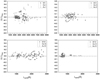 |
Fig. 3 Deviation between HFR and experimental wavelengths, Δλ/λExp (Δλ = λHFR − λExp) as a function of λHFR for spectral lines in Hf I–IV, Os I–IV, and Au I–IV ions. Experimental data were taken from Kramida et al. (2023) (NIST) for Hf I–II, Os III, and Au I; from Malcheva et al. (2009) for Hf III; from Sugar et al. (1974) for Hf IV; from Ivarsson et al. (2003) and Quinet et al. (2006) for Os I; from Ivarsson et al. (2004) and Quinet et al. (2006) for Os II; from Ryabtsev et al. (1998) for Os IV; from Ryabtsev et al. (1998) for Au II; from Zainab & Tauheed (2019) for Au III; and from Wyart et al. (1994) for Au IV. |
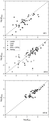 |
Fig. 4 Comparison between HFR oscillator strengths (log gf) and previously published values for Hf I–III ions. Previous data were taken from Duquette et al. (1986) for Hf I and from Den Hartog et al. (2021), Lawler et al. (2007), Lundqvist et al. (2006), and Bouazza et al. (2015) for Hf II. Two different semi-empirical approaches were used in the latter reference based on a parametrization of the oscillator strengths (OSP) and on a pseudo-relativistic Hartree-Fock model including core-polarization effects HFR+CPOL from Malcheva et al. (2009) for Hf III, respectively. |
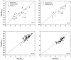 |
Fig. 5 Comparison between HFR oscillator strengths (log gf) and previously published values for Os I–IV ions. Previous data were taken from Quinet et al. (2006), Ivarsson et al. (2003), and Kurucz (1993) for Os I, from Quinet et al. (2006) and Ivarsson et al. (2004) for Os II, from Azarov et al. (2018) for Os III, and from Ryabtsev et al. (1998) for Os IV. |
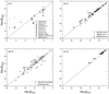 |
Fig. 6 Comparison between HFR oscillator strengths (log gf) and previously published values for Au I–IV ions. Previous data were taken from the NIST database by Kramida et al. (2023), Hannaford et al. (1981), Corliss et al. (1981), Gaarde et al. (1994), Fivet et al. (2007), Desclaux et al. (1994), McCann et al. (2022), Migdalek & Baylis (1979), Migdalek & Garmulewicz (2000), Safronova & Johnson (2004), and Zhang et al. (2018) for Au I; from McCann et al. (2022), Biémont et al. (2007), and Zhang et al. (2002) for Au II; from Zainab & Tauheed (2019) and Enzonga et al. (2008) for Au III; and from Wyart et al. (1994) for Au IV. |
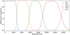 |
Fig. 7 Relative ionic abundances for Hf I–V species as a function of temperature. |
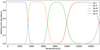 |
Fig. 8 Relative ionic abundances for Os I–V species as a function of temperature. |
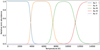 |
Fig. 9 Relative ionic abundances for Au I–V species as a function of temperature. |
3 Opacities
The expansion opacities corresponding to the hafnium, osmium, and gold ions of interest were calculated using the bound-bound absorption coefficient given by (Karp et al. 1977; Eastman & Pinto 1993; Kasen et al. 2006):
![Mathematical equation: $\[\kappa^{bb}(\lambda)=\frac{1}{\rho c t} \sum_l \frac{\lambda_l}{\Delta \lambda}\left(1-\mathrm{e}^{-\tau_l}\right),\]$](/articles/aa/full_html/2024/07/aa48919-23/aa48919-23-eq1.png) (1)
(1)
where λ (in Å) is the central wavelength within the region of width Δλ, λl are the wavelengths of the lines appearing in this range, c (in cm s−1) is the speed of light, ρ (in g cm−3) is the density of the ejected gas, t (in s) is the elapsed time since the ejection, and τl are the optical depths that can be estimated using the Sobolev expression (Sobolev 1960):
![Mathematical equation: $\[\tau_l=\frac{\pi \mathrm{e}^2}{m_e c} f_l n_l t \lambda_l,\]$](/articles/aa/full_html/2024/07/aa48919-23/aa48919-23-eq2.png) (2)
(2)
where e (in C) is the elementary charge, me (in g) is the electron mass, fl (dimensionless) is the oscillator strength, and nl (in cm−3) is the density of the lower level of the transition. The latter can be estimated by assuming the local thermodynamic equilibrium (LTE) through the relation
![Mathematical equation: $\[n_l=\frac{g_l}{U(T)} n \mathrm{e}^{-E_l / k_{\mathrm{B}} T},\]$](/articles/aa/full_html/2024/07/aa48919-23/aa48919-23-eq3.png) (3)
(3)
in which gl and El (in cm−1) are the statistical weight and the energy of the lower level of the transition, respectively, U(T) is the partition function of the ionization stage considered, and n is the ion density evaluated by
![Mathematical equation: $\[n=\frac{\rho}{A m_p} X_j,\]$](/articles/aa/full_html/2024/07/aa48919-23/aa48919-23-eq4.png) (4)
(4)
where A is the mass number, mp is the proton mass, and Xj is the relative ionic fraction of the jth ionization state.
The temperature range in which the Hf I–IV, Os I–IV, and Au I–IV ions contribute the most to the plasma ionic abundances was determined from the Saha equation, in which the relevant partition functions U(T) were computed using all the energy levels obtained in our HFR models described in Sec. 2, completed by Hf V, Os V, and Au V energy levels estimated from HFR calculations including the following configurations: 4f14, 4f13ns (n = 6–8), 4f13np (n = 6–8), 4f13nd (n = 5–8), 4f126s2, 4f125d2, 4f12 5d6s, 4f126s6p for Hf V, 5d4, 5d3ns (n = 6–8), 5d3np (n = 6–8), 5d3nd (n = 6–8), 5d3nf (n = 5–8), 5d26s2, 5d26p2, 5d26d2, 5d25f2, 5d26sns (n = 7–8), 5d26snp (n = 6–8), 5d26snd (n = 6–8), 5d26snf (n = 5–8), 5d26pns (n = 7–8), 5d26pnp (n = 7–8), 5d26pnd (n = 6–8), 5d26pnf (n = 5–8), 5d6s2ns (n = 7–8), 5d6s2np (n = 6–8), 5d6s2nd (n = 6–8) for Os V, and 5d7, 5d6ns (n = 6–8), 5d6np (n = 6–8), 5d6nd (n = 6–8), 5d6nf (n = 5–8), 5d56s2, 5d56p2, 5d55f2, 5d56s6p, 5d56s5f, 5d56s6f, 5d56p5f for Au V. The ionization potentials were taken from the NIST database (Kramida et al. 2023). This gave rise to the ionization balances as shown in Figs. 7–9 for the first ions of hafnium, osmium, and gold, respectively. From these figures, we deduced that the maximum relative abundances occurred at T = 2000 K for Hf I, Os I, and Au I; T = 4000 K for Hf II; T = 5000 K for Os II; T = 6000 K for Au II; T = 7500 K for Hf III; T = 8000 K for Os III; T = 10000 K for Au III; T = 11000 K for Hf IV; T = 12 500 K for Os IV; and T = 15 000 K for Au IV. We therefore limited the opacity calculations to the temperature range not exceeding 15000 K.
The expansion opacities were computed using all the electric dipole transitions for which the upper level was below the ionization potential and the log gf-value was greater than −5. This led to a very large amount of transitions for each element (see Table 1). It is important to note that these numbers are much higher than the numbers of transitions included in the opacity calculations of Tanaka et al. (2020), which considered a total of about 385 000 lines for the 12 atomic systems of interest, to be compared with a total of slightly over 18 million in our work (i.e., a number of lines 50 times greater). In all of our computations, the elapsed time after NS merger was assumed to be t = 1 day, and the density of the gas was chosen to be ρ = 10−13 g cm−3, as suggested by Banerjee et al. (2022), for example, while the width of wavelength bin was set at Δλ = 10 Å.
The results obtained are shown in Figs. 10–12, where the calculated expansion opacities of hafnium, osmium, and gold are compared for three different temperatures, namely T = 5000 K, T = 10 000 K, and T = 15 000 K, respectively. We can clearly see that the contribution of Os is much more significant than that of Hf and Au for the first two temperatures, as highlighted by Tanaka et al. (2020).
A commonly used wavelength-independent absorption coefficient is the Planck mean opacity, κp, which is the integrated opacity related to the total radiation absorbed and defined as
![Mathematical equation: $\[\kappa_P(T)=\frac{\int_0^{\infty} B(\lambda, T) ~\kappa(\lambda) \mathrm{~d} \lambda}{\int_0^{\infty} B(\lambda, T) \mathrm{~d} \lambda},\]$](/articles/aa/full_html/2024/07/aa48919-23/aa48919-23-eq5.png) (5)
(5)
where B(λ,T) is the Planck function given by
![Mathematical equation: $\[B(\lambda, T)=\frac{2 h c^2}{\lambda^5} \frac{1}{\mathrm{e}^{h c / \lambda k T}-1}.\]$](/articles/aa/full_html/2024/07/aa48919-23/aa48919-23-eq6.png) (6)
(6)
The Planck mean opacities computed in the present work are plotted in Fig. 13 for temperatures up to 15 000 K. As seen from this figure, at the lowest temperature, T = 3000 K, hafmium and osmium produce an opacity two orders of magnitude higher than gold. When the temperature increases, if Os always remains the main contributor, the opacity of Hf decreases while that of gold increases until both elements have a similar contribution around T = 10 000 K. At 15 000 K, osmium contribution to the Plank mean opacity is about four times higher than gold contribution, which is itself about four times greater than that of hafnium. Overall, these results are in fairly good agreement with the Planck mean opacities roughly extracted from Fig. 7 of Tanaka et al. (2020), even if the values of the latter seem a factor of 2–3 smaller than our results for osmium at 5000 K and for hafnium at 15 000 K. This could be due to the differences between the atomic models used, those considered in our work giving rise to many more radiative transitions that can contribute to monochromatic opacities. This point was already mentioned in Sec. 2 and highlighted in Figs. 1 and 2, where comparisons of the level densities obtained in our calculations and those deduced from Tanaka et al. (2020) are given, showing (sometimes rather large) differences for the Hf I–IV, Os I–IV, and Au I–IV ions considered.
It is, however, worth highlighting that the opacities determined in the present work were computed assuming singleelement plasma for each species; that is, they do not take the elemental abundances within the kilonova ejecta into account. Determining the contribution of each species to the total ejecta opacity would require a realistic estimate of their corresponding abundance, which could be obtained from NS merger simulations. This will be within the scope of a further investigation in which all elements and their abundances will be included in order to estimate their respective contributions to the kilonova ejecta total opacity.
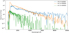 |
Fig. 10 Expansion opacity for Hf, Os, and Au, calculated at T = 5000 K. |
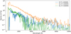 |
Fig. 11 Expansion opacity for Hf, Os, and Au, calculated at T = 10 000 K. |
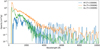 |
Fig. 12 Expansion opacity for Hf, Os, and Au, calculated at T = 15 000 K. |
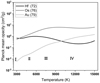 |
Fig. 13 Planck mean opacities for Hf, Os, and Au as a function of temperature. The labels I, II, III, and IV show typical temperature ranges for each ionization state. |
4 Summary and conclusion
New calculations of the atomic structures and radiative parameters for a very large number of spectral lines were carried out in the charge stages I–IV of three elements of the sixth period, Hf, Os, and Au. To do this, we used the pseudo-relativistic Hartree–Fock theoretical method including a large amount of electronic configurations. These ab initio atomic data were found to be generally in good agreement with previously published experimental and theoretical results. The reliability of our atomic parameters and especially their quantity, with approximately 0.5 million, 16 million, and 1.2 million radiative transitions computed in Hf, Os, and Au ions, respectively, allowed us to estimate the expansion and Planck opacities corresponding to ejecta conditions expected one day after a neutron star merger (i.e., T ~ 5000–15000 K and ρ ~ 10−13 g cm−3). It was shown that, due to its very high spectral density, Os is the main contributor to Planck mean opacity over the entire temperature range, while the contributions of Hf and Au reverse as the temperature increases. This is because the Planck mean opacity of Au is about four times greater than that of Hf at T = 15 000 K, while it is two orders of magnitude lower than the one of Hf at T = 5000 K. Of course, these different contributions must be weighted by the respective chemical abundances to estimate the total opacities affecting the kilonova spectra.
Acknowledgements
H.C.G. is holder of a FRIA fellowship while P.P. and P.Q. are, respectively, Research Associate and Research Director of the Belgian Fund for Scientific Research F.R.S.-FNRS. This project has received funding from the FWO and F.R.S.-FNRS under the Excellence of Science (EOS) programme (Grant Nos. O.0228.18 and O.0004.22). Part of the atomic calculations were made with computational resources provided by the Consortium des Équipements de Calcul Intensif (CECI), funded by the F.R.S.-FNRS under Grant No. 2.5020.11 and by the Walloon Region of Belgium.
Appendix A Additional tables
Configurations included in HFR atomic structure calculations for Hf I-IV ions.
Configurations included in HFR atomic structure calculations for Os I-IV ions.
Configurations included in HFR atomic structure calculations for Au I-IV ions.
Comparison between available experimental values of the first few excited energy levels in Hf I–IV and the HFR results obtained without scaling down the Slater integrals (SF = 1.00) and with a scaling factor of 0.85 (SF = 0.85).
Comparison between available experimental values of the first few excited energy levels in Os I–IV and the HFR results obtained without scaling down the Slater integrals (SF = 1.00) and with a scaling factor of 0.85 (SF = 0.85).
Comparison between available experimental values of the first few excited energy levels in Au I–IV and the HFR results obtained without scaling down the Slater integrals (SF = 1.00) and with a scaling factor of 0.85 (SF = 0.85).
References
- Ankita, S., & Tauheed, A. 2018, JQSRT, 05, 022 [Google Scholar]
- Ankita, S., & Tauheed, A. 2020, JQSRT, 254, 107193 [NASA ADS] [CrossRef] [Google Scholar]
- Azarov, V. I., Tchang-Brillet, W.-Ü. L., & Gayasov, R. R. 2018, At. Data Nucl. Data Tables, 121, 345 [CrossRef] [Google Scholar]
- Banerjee, S., Tanaka, M., Kawaguchi, K., Kato, D., & Gaigalas, G. 2020, ApJ, 901, 29 [NASA ADS] [CrossRef] [Google Scholar]
- Banerjee, S., Tanaka, M., Kato, D., et al. 2022, ApJ, 934, 117 [CrossRef] [Google Scholar]
- Banerjee, S., Tanaka, M., Kato, D., & Gaigalas, G. 2024, ApJ, 968, 64 [NASA ADS] [CrossRef] [Google Scholar]
- Beck, D. R., & Pan, L. 2004, Phys. Scr., 69, 91 [NASA ADS] [CrossRef] [Google Scholar]
- Ben Nasr, S., Carvajal Gallego, H., Deprince, J., Palmeri, P., & Quinet, P. 2023, A&A, 678, A67 [NASA ADS] [CrossRef] [EDP Sciences] [Google Scholar]
- Biémont, E., Blagoev, K., Fivet, V., et al. P. 2007, MNRAS, 380, 1581 [CrossRef] [Google Scholar]
- Bouazza, S., Quinet, P., & Palmeri, P. 2015, JQSRT, 163, 39 [NASA ADS] [CrossRef] [Google Scholar]
- Carvajal Gallego, H., Palmeri, P., & Quinet, P. 2021, MNRAS, 501, 1440 [Google Scholar]
- Carvajal Gallego, H., Berengut, J. C., Palmeri, P., & Quinet, P. 2022a, MNRAS, 509, 6138 [Google Scholar]
- Carvajal Gallego, H., Berengut, J. C., Palmeri, P., & Quinet, P. 2022b, MNRAS, 513, 2302 [NASA ADS] [CrossRef] [Google Scholar]
- Carvajal Gallego, H., Deprince, J., Berengut, J. C., Palmeri, P., & Quinet, P. 2023a, MNRAS, 518, 332 [Google Scholar]
- Carvajal Gallego, H., Deprince, J., Palmeri, P., & Quinet, P. 2023b, MNRAS, 522, 312 [NASA ADS] [CrossRef] [Google Scholar]
- Carvajal Gallego, H., Deprince, J., Godefroid, M., et al. 2023c, Eur. Phys. J. D, 77, 72 [NASA ADS] [CrossRef] [Google Scholar]
- Corliss, C. H., & Bozman W. R. 1962, Experimental Transition Probabilities for Spectral Lines of Seventy Elements (NBS Monograph 53) (Washington, DC: US Govt Printing Office), 7 [Google Scholar]
- Cowan, R. D. 1981, The Theory of Atomic Structure and Spectra (Berkeley: California University Press) [Google Scholar]
- Den Hartog, E. A., Lawler, J. E., & Roederer, I. U. 2021, ApJS, 254, 5 [NASA ADS] [CrossRef] [Google Scholar]
- Deprince, J., Carvajal Gallego, H., Godefroid, M., et al. 2023, Eur. Phys. J. D, 77, 93 [NASA ADS] [CrossRef] [Google Scholar]
- Desclaux, J. P., & Kim, Y.-K. 1975, J. Phys. B, 8, 1177 [NASA ADS] [CrossRef] [Google Scholar]
- Duquette, D. W., Den Hartog, E. A., & Lawler, J. E. 1986, JQSRT, 35, 281 [NASA ADS] [CrossRef] [Google Scholar]
- Eastman, R. G., & Pinto, P. A. 1993, ApJ, 412, 731 [NASA ADS] [CrossRef] [Google Scholar]
- Eichler, D., Livio, M., Piran, T., & Schramm, D. N. 1989, Nature, 340, 126 [NASA ADS] [CrossRef] [Google Scholar]
- Enzonga Yoca, S., Biémont, E., Delahaye, F., Quinet, P., & Zeippen, C. J. 2008, Phys. Scr., 78, 025303 [NASA ADS] [CrossRef] [Google Scholar]
- Fivet, V., Quinet, P., Palmeri, P., Biémont, E., & Xu, H. L. 2007, J. Elect. Spectr. Rel. Phen., 250 [CrossRef] [Google Scholar]
- Flörs, A., Silva, R. F., Deprince, J., et al. 2023, MNRAS, 524, 3083 [CrossRef] [Google Scholar]
- Fontes, C. J., Fryer, C. L., Hungerford, A. L., Wollaeger, R. T., & Korobkin, O. 2020, MNRAS, 493, 4143 [CrossRef] [Google Scholar]
- Fontes, C. J., Fryer, C. L., Wollaeger, R. T., Mimpower, M. R., & Sprouse, T. M. 2023, MNRAS 519, 2862 [Google Scholar]
- Freiburghaus, C., Rosswog, S., & Thielemann, F. K. 1999, ApJ, 525, L121 [NASA ADS] [CrossRef] [Google Scholar]
- Gaarde, M. B., Zerne, R., Caiyan, L., et al. 1994, Phys. Rev. A, 50, 209 [NASA ADS] [CrossRef] [Google Scholar]
- Gaigalas, G., Kato, D., Rynkun, P., Radžiūtė, L., & Tanaka, M. 2019, ApJS, 240, 29 [NASA ADS] [CrossRef] [Google Scholar]
- Gaigalas, G., Rynkun, P., Radžiūtė, L., et al. 2020, ApJS, 248, 13 [CrossRef] [Google Scholar]
- Gao, Y., Geng, Y., Quinet, P., et al. 2019, ApJS, 242, 23 [NASA ADS] [CrossRef] [Google Scholar]
- Glowacki, L., & Migdalek, J. 2009, Phys. Rev. A, 80, 042505 [NASA ADS] [CrossRef] [Google Scholar]
- Hannaford, P., Larkins, P. L., & Lowe, R. M. 1981, J. Phys. B, At. Mol. Phys., 14, 2321 [NASA ADS] [CrossRef] [Google Scholar]
- Ivarsson, S., Andersen, J., Nordström, B., et al. 2003, A&A, 409, 1141 [NASA ADS] [CrossRef] [EDP Sciences] [Google Scholar]
- Ivarsson, S., Wahlgren, G. M., Dai, Z., Lundberg, H., & Leckrone, D. S. 2004, A&A, 425, 353 [NASA ADS] [CrossRef] [EDP Sciences] [Google Scholar]
- Just, O., Kullmann, I., Goriely, S., et al. 2022, MNRAS, 510, 2820 [NASA ADS] [CrossRef] [Google Scholar]
- Karp, A. H., Lasher, G., Chan, K. L., & Salpeter, E. E. 1977, ApJ, 214, 161 [NASA ADS] [CrossRef] [Google Scholar]
- Kasen, D., Thomas, R. C., & Nugent, P. 2006, ApJ, 651, 366 [NASA ADS] [CrossRef] [Google Scholar]
- Kasen, D., Badnell, N. R., & Barnes, J. 2013, ApJ, 774, 25 [NASA ADS] [CrossRef] [Google Scholar]
- Kasen, D., Metzger, B., Barnes, J., Quataert, E., & Ramirez-Ruiz, E. 2017, Nature, 551, 80 [Google Scholar]
- Korobkin, O., Rosswog, S., Arcones, A., & Winteler, C. 2012, MNRAS, 426, 1940 [NASA ADS] [CrossRef] [Google Scholar]
- Kramida, A., Ralchenko, Yu., Reader, J., & NIST ASD Team 2023, NIST Atomic Database, National Institute of Standards and Technology, Gaithersburg, MD, https://physics.nist.gov/asd [Google Scholar]
- Kurucz, R. L. 1993, Synthesis Programs and Line Data (Kurucz CD-ROM No. 18) [Google Scholar]
- Lattimer, J. M., & Schramm, D. N. 1974, ApJ, 192, L145 [NASA ADS] [CrossRef] [Google Scholar]
- Lawler, J. E., Den Hartog, E. A., & Labby, Z. E. 2007, ApJS, 169, 120 [NASA ADS] [CrossRef] [Google Scholar]
- Lundqvist, M., Nilsson, H., Wahlgren, G. M., et al. 2006, A&A, 450, 407 [NASA ADS] [CrossRef] [EDP Sciences] [Google Scholar]
- Maison, L., Carvajal Gallego, H., & Quinet, P. 2022, Atoms, 10, 130 [CrossRef] [Google Scholar]
- Malcheva, G., Enzonga Yoca, S., Mayo, R., et al. 2009, MNRAS, 396, 2289 [NASA ADS] [CrossRef] [Google Scholar]
- McCann, M., Bromley, S., Loch, S. D., & Ballance, C. P. 2022, MNRAS, 509, 4723 [Google Scholar]
- Metzger, B. D. 2017, Living Rev. Relativ, 20, 3 [NASA ADS] [CrossRef] [Google Scholar]
- Metzger, B. D., Martínez-Pinedo, G., Darbha, S., et al. 2010, MNRAS, 406, 2650 [NASA ADS] [CrossRef] [Google Scholar]
- Migdalek, J., & Baylis, W. E. 1979, JQSRT, 22, 113 [NASA ADS] [CrossRef] [Google Scholar]
- Migdalek, J., & Baylis, W. E. 1987, JQSRT, 31, 521 [NASA ADS] [CrossRef] [Google Scholar]
- Migdalek, J., & Garmulewicz, M. 2000, J. Phys. B, 33, 1735 [NASA ADS] [CrossRef] [Google Scholar]
- Nilsson, H., Hartman, H., Engström, L., et al. 2010, A&A, 511, A16 [NASA ADS] [CrossRef] [EDP Sciences] [Google Scholar]
- Perego, A., Radice, D., & Bernuzzi, S. 2017, ApJ, 850, L37 [NASA ADS] [CrossRef] [Google Scholar]
- Pickering, J. C., & Zilio, V. 2001, Eur. Phys. J. D, 181, 13 [Google Scholar]
- Quinet, P., Palmeri, P., Biémont, E., et al. 2006, A&A, 448, 1207 [NASA ADS] [CrossRef] [EDP Sciences] [Google Scholar]
- Radžiūtė, L., Gaigalas, G., Kato, D., Rynkun, P., & Tanaka, M. 2020, ApJS, 248, 17 [CrossRef] [Google Scholar]
- Radžiūtė, L., Gaigalas, G., Kato, D., Rynkun, P., & Tanaka, M. 2021, ApJS, 257, 29 [CrossRef] [Google Scholar]
- Rosberg, M., & Wyart, J. F. 1997, Phys. Scr., 55, 690 [NASA ADS] [CrossRef] [Google Scholar]
- Rosswog, S. 2015, Int. J. Mod. Phys. D, 24, 1530012 [NASA ADS] [CrossRef] [Google Scholar]
- Ruczkowski, J., Bouazza, S., Elantkowska, M., & Dembczyński, J. 2015, JQSRT, 155, 1 [NASA ADS] [CrossRef] [Google Scholar]
- Ruczkowski, J., Elantkowska, M., & Dembczynski, J. 2016, MNRAS, 459, 3768 [NASA ADS] [CrossRef] [Google Scholar]
- Ryabtsev, A. N., Raassen, A. J. J., Tchang-Brillet, W.-Ü. L., et al. 1998, Phys. Scr., 57, 82 [CrossRef] [Google Scholar]
- Rynkun, P., Banerjee, S., Gaigalas, G., et al. 2022, A&A, 658, A82 [NASA ADS] [CrossRef] [EDP Sciences] [Google Scholar]
- Safronova, U. I., & Johnson, W. R. 2004, Phys. Rev. A, 69, 052511 [NASA ADS] [CrossRef] [Google Scholar]
- Safronova, U. I., Johnson, W. R., & Safronova, M. S. 2002, Phys. Rev. A, 66, 022507 [NASA ADS] [CrossRef] [Google Scholar]
- Sobolev, V. V. 1960, Moving Envelopes of Stars (Cambridge, MA: Harvard Univ. Press) [Google Scholar]
- Sugar, J., & Kaufman, V. 1974, J. Opt. Soc. Am., 64, 1656 [NASA ADS] [CrossRef] [Google Scholar]
- Tanaka, M., Kato, D., Gaigalas, G., & Kawaguchi K. 2020, MNRAS, 496, 1369 [NASA ADS] [CrossRef] [Google Scholar]
- Tauheed, A., & Reader, J. 2005, Phys. Scr., 72, 158 [NASA ADS] [CrossRef] [Google Scholar]
- Villar, V. A., Guillochon, J., Berger, E., et al. 2017, ApJ, 851, L21 [Google Scholar]
- Wanajo, S., Sekiguchi, Y., Nishimura, N., et al. 2014, ApJ, 789, L39 [Google Scholar]
- Wyart, J. F., Joshi, Y. N., Raasen, A. J. J., et al. 1994, Phys. Scr., 50, 672 [NASA ADS] [CrossRef] [Google Scholar]
- Zainab, A., & Tauheed, A. 2019, JQSRT, 237, 106614 [NASA ADS] [CrossRef] [Google Scholar]
- Zainab, A., Haris, K., Gamrath, S., Quinet, P., & Tauheed, A. 2023, ApJS, 267, 12 [NASA ADS] [CrossRef] [Google Scholar]
- Zhang, Z., Brage, T., Curtis, L. J., Lundberg, H., & Martinson, I. 2002, J. Phys. B: At. Mol. Opt. Phys., 35, 483 [NASA ADS] [CrossRef] [Google Scholar]
- Zhang, W., Palmeri, P., & Quinet, P. 2013, Phys. Scr, 88, 065302 [NASA ADS] [CrossRef] [Google Scholar]
- Zhang, M., Zhou, L., Gao, Y., et al. 2018, J. Phys. B: At. Mol. Opt. Phys., 51, 205001 [NASA ADS] [CrossRef] [Google Scholar]
All Tables
Number of levels and transitions obtained with HFR calculations and used for opacity determination in Hf, Os, and Au I–IV ions.
Comparison between available experimental values of the first few excited energy levels in Hf I–IV and the HFR results obtained without scaling down the Slater integrals (SF = 1.00) and with a scaling factor of 0.85 (SF = 0.85).
Comparison between available experimental values of the first few excited energy levels in Os I–IV and the HFR results obtained without scaling down the Slater integrals (SF = 1.00) and with a scaling factor of 0.85 (SF = 0.85).
Comparison between available experimental values of the first few excited energy levels in Au I–IV and the HFR results obtained without scaling down the Slater integrals (SF = 1.00) and with a scaling factor of 0.85 (SF = 0.85).
All Figures
|
Fig. 1 Comparison between full set of HFR energy levels calculated using the physical models of the present work (in black) and the HFR energy levels obtained using the physical models considered by Tanaka et al. (2020) (in blue) for Hf I–IV, Os I–IV, and Au I–IV. The red lines correspond to the ionization potentials taken from the NIST database (Kramida et al. 2023). |
| In the text | |
|
Fig. 2 Comparison between full set of HFR energy levels calculated using physical models of present work (in black) and HFR energy levels obtained using physical models considered by Tanaka et al. (2020) (in blue) for Os II between 120 000 and 138 000 cm−1. The red line corresponds to the ionization potential taken from the NIST database (Kramida et al. 2023). |
| In the text | |
|
Fig. 3 Deviation between HFR and experimental wavelengths, Δλ/λExp (Δλ = λHFR − λExp) as a function of λHFR for spectral lines in Hf I–IV, Os I–IV, and Au I–IV ions. Experimental data were taken from Kramida et al. (2023) (NIST) for Hf I–II, Os III, and Au I; from Malcheva et al. (2009) for Hf III; from Sugar et al. (1974) for Hf IV; from Ivarsson et al. (2003) and Quinet et al. (2006) for Os I; from Ivarsson et al. (2004) and Quinet et al. (2006) for Os II; from Ryabtsev et al. (1998) for Os IV; from Ryabtsev et al. (1998) for Au II; from Zainab & Tauheed (2019) for Au III; and from Wyart et al. (1994) for Au IV. |
| In the text | |
|
Fig. 4 Comparison between HFR oscillator strengths (log gf) and previously published values for Hf I–III ions. Previous data were taken from Duquette et al. (1986) for Hf I and from Den Hartog et al. (2021), Lawler et al. (2007), Lundqvist et al. (2006), and Bouazza et al. (2015) for Hf II. Two different semi-empirical approaches were used in the latter reference based on a parametrization of the oscillator strengths (OSP) and on a pseudo-relativistic Hartree-Fock model including core-polarization effects HFR+CPOL from Malcheva et al. (2009) for Hf III, respectively. |
| In the text | |
|
Fig. 5 Comparison between HFR oscillator strengths (log gf) and previously published values for Os I–IV ions. Previous data were taken from Quinet et al. (2006), Ivarsson et al. (2003), and Kurucz (1993) for Os I, from Quinet et al. (2006) and Ivarsson et al. (2004) for Os II, from Azarov et al. (2018) for Os III, and from Ryabtsev et al. (1998) for Os IV. |
| In the text | |
|
Fig. 6 Comparison between HFR oscillator strengths (log gf) and previously published values for Au I–IV ions. Previous data were taken from the NIST database by Kramida et al. (2023), Hannaford et al. (1981), Corliss et al. (1981), Gaarde et al. (1994), Fivet et al. (2007), Desclaux et al. (1994), McCann et al. (2022), Migdalek & Baylis (1979), Migdalek & Garmulewicz (2000), Safronova & Johnson (2004), and Zhang et al. (2018) for Au I; from McCann et al. (2022), Biémont et al. (2007), and Zhang et al. (2002) for Au II; from Zainab & Tauheed (2019) and Enzonga et al. (2008) for Au III; and from Wyart et al. (1994) for Au IV. |
| In the text | |
|
Fig. 7 Relative ionic abundances for Hf I–V species as a function of temperature. |
| In the text | |
|
Fig. 8 Relative ionic abundances for Os I–V species as a function of temperature. |
| In the text | |
|
Fig. 9 Relative ionic abundances for Au I–V species as a function of temperature. |
| In the text | |
|
Fig. 10 Expansion opacity for Hf, Os, and Au, calculated at T = 5000 K. |
| In the text | |
|
Fig. 11 Expansion opacity for Hf, Os, and Au, calculated at T = 10 000 K. |
| In the text | |
|
Fig. 12 Expansion opacity for Hf, Os, and Au, calculated at T = 15 000 K. |
| In the text | |
|
Fig. 13 Planck mean opacities for Hf, Os, and Au as a function of temperature. The labels I, II, III, and IV show typical temperature ranges for each ionization state. |
| In the text | |
Current usage metrics show cumulative count of Article Views (full-text article views including HTML views, PDF and ePub downloads, according to the available data) and Abstracts Views on Vision4Press platform.
Data correspond to usage on the plateform after 2015. The current usage metrics is available 48-96 hours after online publication and is updated daily on week days.
Initial download of the metrics may take a while.