| Issue |
A&A
Volume 707, March 2026
|
|
|---|---|---|
| Article Number | A172 | |
| Number of page(s) | 13 | |
| Section | Cosmology (including clusters of galaxies) | |
| DOI | https://doi.org/10.1051/0004-6361/202558242 | |
| Published online | 03 March 2026 | |
The AIDA-TNG project: Abundance, radial distribution, and clustering properties of halos in alternative dark matter models
1
Dipartimento di Fisica e Astronomia “A. Righi” – Alma Mater Studiorum Università di Bologna via Piero Gobetti 93/2 40129 Bologna, Italy
2
INAF – Osservatorio di Astrofisica e Scienza dello Spazio di Bologna via Piero Gobetti 93/3 40129 Bologna, Italy
3
INFN – Sezione di Bologna Viale Berti Pichat 6/2 40127 Bologna, Italy
4
Department of Physics, Kavli Institute for Astrophysics and Space Research, Massachusetts Institute of Technology Cambridge MA 02139, USA
★ Corresponding author: This email address is being protected from spambots. You need JavaScript enabled to view it.
Received:
24
November
2025
Accepted:
26
January
2026
Abstract
Warm and self-interactive dark matter cosmologies have been proposed as nonbaryonic solutions to the tensions between the Λ cold dark matter model and observations at the kiloparsec scale. In this paper, we used the dark matter-only runs of the AIDA-TNG project, a set of cosmological simulations of different sizes and resolutions, to analyze the macroscopic impact of alternative dark matter models on the abundance, radial distribution, and clustering properties of halos. We adopted the halo occupation distribution formalism to characterize the evolution of its parameters M1 and α with the mass and redshift selection of our sample. By dividing the halo population into centrals and satellites, we were able to study their spatial density profile. We found that a Navarro-Frenk-White model is not accurate enough to describe the radial distribution of subhalos and that a generalized Navarro-Frenk-White model is required instead. Warm dark matter models, in particular, present a cuspier distribution of satellites, whereas self-interacting dark matter exhibits a shallower density profile. Moreover, we found that the small-scale clustering of dark matter halos provides a powerful tool for distinguishing among alternative dark matter scenarios, in preparation for a more detailed study that fully incorporates baryonic effects and for a comparison with observational data from galaxy clustering.
Key words: galaxies: abundances / galaxies: halos / cosmology: theory / large-scale structure of Universe
© The Authors 2026
 Open Access article, published by EDP Sciences, under the terms of the Creative Commons Attribution License (https://creativecommons.org/licenses/by/4.0), which permits unrestricted use, distribution, and reproduction in any medium, provided the original work is properly cited.
This article is published in open access under the Subscribe to Open model. This email address is being protected from spambots. You need JavaScript enabled to view it. to support open access publication.
1. Introduction
In the past decades, a significant part of the cosmological investigation has been dedicated to shedding light on the central topic of the origin and the growth of cosmic structures. These efforts led to the formulation of the so-called hierarchical model of structure formation (White & Rees 1978). According to this, structure formation is the result of the growth of primordial overdensities in the matter distribution that arise at the end of the inflationary era from initial quantum fluctuations in the early Universe. In this framework, gravitationally bound systems, such as galaxies and galaxy clusters, are the product of gravitational infall, the progressive merging of dark matter halos, and the catching up of baryons (White & Rees 1978; Bardeen et al. 1986; Tormen 1998).
Several physical processes contribute to the formation and assembly history of these complex systems. Among them, the long-range nonlinear gravitational interaction sets the dynamic of the overall matter distribution, while different radiative processes, including stellar emission and gas cooling, affect the baryonic matter in different phases. Finally, a series of feedback phenomena, such as supernova explosions (Efstathiou 2000; Smith et al. 2018), stellar winds (Springel & Hernquist 2003; Davé et al. 2011; Hopkins et al. 2012), and active galactic nucleus emission (Bower et al. 2006; Weinberger et al. 2018), reshape the matter distribution as well as the star formation rate (Scharré et al. 2024). Due to the large number of interactions and physical processes involved, an analytical treatment of structure formation is currently unfeasible.
For this reason, numerical simulations have been developed in a wide range of sizes and resolutions that target well-defined scientific cases. They offer important tools for investigating the statistical properties of cosmological systems and testing models that will be applied to observations and real datasets. In particular, for a given set of cosmological parameters, N-body simulations trace the evolution of the dark component alone, following the gravitational interaction of dark matter particles over cosmic time (Springel et al. 2001b; Springel 2005), while hydrodynamical simulations also include baryons, allowing us to understand the complex interplay between their different components, such as gas, stars, and black holes (Duffy et al. 2010; Vogelsberger et al. 2014a; Chisari et al. 2018; Springel et al. 2018; Vogelsberger et al. 2020).
The clustering of large-scale structure (LSS) is recognized today as a fundamental cosmological probe because during different periods of the cosmic expansion, it keeps the memory of the footprint left by the initial conditions of the Universe. In practice, this offers us the possibility to provide constraints on the main cosmological parameters, such as the matter density content of the Universe and the normalization of the primordial fluctuations (Hildebrandt et al. 2020; Asgari et al. 2021; Abbott et al. 2022; Amon et al. 2022; Lesci et al. 2022; Secco et al. 2022; Romanello et al. 2024). In addition, the clustering of LSS is typically combined with other cosmological probes, such as number counts of cosmic structures (To et al. 2021), or a simultaneous study of different two-point statistics (Heymans et al. 2021), which includes cosmic shear (Kilbinger 2015; Hildebrandt et al. 2020; Asgari et al. 2021) and galaxy–galaxy lensing, and can potentially highlight differences in the concordance cosmological paradigm.
Currently, the most widely acknowledged cosmological scenario is the Λ cold dark matter (ΛCDM) model, which assumes that dark matter particles are in a ‘cold’ version, namely in the form of very massive nonrelativistic candidates, such as weakly interacting massive particles, with a mass mX > 1 GeV, or condensates of light axions, with mX ≲ 10−3 eV (Strigari 2013). The ΛCDM model is consistent with observations at various scales that range from the typical intergalactic distances to the size of the cosmological horizon. It also provides robust explanations for observations of the cosmic microwave background, for the abundances of light elements as products of the primordial nucleosynthesis, and for the accelerating expansion of the Universe. Moreover, it reasonably describes the distribution and statistical properties of the LSS.
However, some possible tensions have been suggested by observations on the galactic and sub-galactic scales, of the order of kiloparsec (see Weinberg et al. 2015; Bullock & Boylan-Kolchin 2017; Del Popolo & Le Delliou 2017 for reviews). Among them, the ‘missing satellites’ (Klypin et al. 1999) and the ‘too-big-to-fail’ problems (Boylan-Kolchin et al. 2011), which are related to the fact that the abundance of satellites around the Milky Way does not match the number of galactic subhalos measured in N-body simulations, and the ‘cusp-core’ problem, which arises because the observed halo density profiles are less concentrated than the predicted cusped Navarro-Frenk-White profiles (NFW, Navarro et al. 1996). Although a recent galactic census has significantly alleviated the missing satellite problem (Kim et al. 2018), the issue remains open scientifically. Usually, baryonic phenomena are invoked as possible solutions (Brooks et al. 2013); for example, photoionization feedback to quench star formation in low-mass halos (Busha et al. 2010; Castellano et al. 2016; Yue et al. 2018), and supernova feedback and tidal stripping to expel gas from the galactic environment, resulting in a redistribution of matter that erases the internal cusps of density profile and in a reduction of the number of faint satellites (Brooks et al. 2013; Bullock & Boylan-Kolchin 2017).
Another perhaps more intriguing possibility is the exploration of the dark sector by investigating the macroscopic consequences of alternative cosmological scenarios that postulate the existence of warm dark matter (WDM, Bode et al. 2001; Viel et al. 2005; Schneider et al. 2012; Lovell et al. 2014) or self-interacting dark matter particles (SIDM, Spergel & Steinhardt 2000; Vogelsberger et al. 2012). In the first case, the growth of cosmic perturbations smaller than a characteristic free streaming length is suppressed by the thermal motion of collisionless dark matter particles. This naturally produces shallower density profiles and fewer low-mass halos (Menci et al. 2016). This observationally translates into a turnover at the faint end of the rest-frame galaxy UV luminosity function (Corasaniti et al. 2017) and in a general delay of galaxy formation (Dayal et al. 2015; Menci et al. 2018), with a possible effect on the timeline of the reionization process (Dayal et al. 2017; Carucci & Corasaniti 2019; Romanello et al. 2021). In the latter case, dark matter particles have a nonzero cross section of self-interaction, σ, which yields a non-negligible scattering probability that allows for a transfer and a redistribution of energy and momentum between different parts of dark matter halos (see Tulin & Yu 2018; Adhikari et al. 2025, for reviews). As a result, the inner region of the density profile tends to become cored and isothermal, whereas the outer part, in which the density and the interaction rate are lower, is well described by an NFW profile. In more realistic SIDM models, self-interaction is determined by a massive mediator and σ decreases with the relative velocities of the interacting particles (Vogelsberger et al. 2012; Correa 2021; Adhikari et al. 2025). Systems such as galaxy clusters, which have a large velocity dispersion, are therefore less affected than faint galaxies. As a consequence, SIDM affects on kiloparsec rather than on megaparsec scales, which agrees with what is expected from the observational evidence in the local Universe.
This publication is part of a series of works that make use of a suite of cosmological simulations (Despali et al. 2025) to study and characterize the properties of dark matter halos, such as their shapes (Giocoli et al. 2026), gas distribution (Zhang et al. 2026), concentrations and density profiles (Despali et al. 2026), in alternative dark matter models. The management of halo catalogs, the measurements of the relevant two-point statistics, the cosmological modeling, and the Bayesian inference presented in this study were performed with COSMOBOLOGNALIB1 (Marulli et al. 2016), a set of free software libraries for C++ and Python.
2. The AIDA-TNG simulations
The AIDA-TNG sample (Alternative Dark Matter in the TNG universe, Despali et al. 2025) is a set of cosmological simulations designed to study the effect of alternative dark matter models (WDM and SIDM) on multiple scales. Boxes of 110.7 and 51.7 Mpc on a side, corresponding to 75 and 35 Mpc h−1, are presented in Despali et al. (2025); we refer to them as “100/” and “50/”. Each box is simulated in up to six dark matter scenarios, as well as with and without baryons, and labeled according to its decreasing mass resolution: mDM = 4.8 × 10⁷ M⊙ h−1 for 100/A, mDM = 2.9 × 10⁶ M⊙ h−1 for 50/A, and 2.3 × 10⁷ M⊙ h−1 for 50/B, respectively. The simulations are listed in Table 1, with respective details and available cosmologies. The baryonic physics is included through the TNG galaxy formation model (Weinberger et al. 2017; Pillepich et al. 2018b).
Overview of the dark matter-only runs of the AIDA-TNG simulations, including box size, dark matter particle mass, and available dark matter models.
The starting redshift of the simulations is z = 127, with initial conditions derived with the Zel’dovich approximation, as also in the IllustrisTNG simulations (Vogelsberger et al. 2014b; Pillepich et al. 2018a). The friends-of-friends (FOF) and SUBFIND algorithms (Springel et al. 2001a) have been used to identify dark matter halos and subhalos, respectively. First, the FOF group finder is run. We then refer to subhalos as sets of locally overdense, gravitationally bound particles that are hosted in each FOF detection. The position of central subhalos coincides with the minimum of the gravitational potential, that is, with the centers of the FOF halo (Pillepich et al. 2018a). Therefore, throughout this paper, we consider satellites and subhalos to be synonyms.
For the purpose of our work, we focus on dark matter-only 50/A and 50/B boxes at z = 2, z = 1, z = 0.5 and z = 0, in order to take advantage of the resolution and of the largest variety of dark matter models, while leaving further study on the baryonic influence to the future. The cosmological parameters of the simulations are taken from Planck Collaboration XXIV (2016): Ωm = 0.3089, ΩΛ = 0.6911, Ωb = 0.0486, H0 = 0.6774, and σ8 = 0.8159.
The AIDA-TNG project explores the same cosmological volumes in different alternative dark matter scenarios. In particular, for WDM cosmologies, dark matter is considered a ‘thermal relic’, resulting from the freeze-out of a dark component in thermal equilibrium with the early Universe. From a physical point of view, the free streaming of dark matter particles determines a suppression in the power spectrum, P(k), which can be modeled through the transfer function, T(k) (Bode et al. 2001; Viel et al. 2005; Schneider et al. 2012),
![Mathematical equation: $$ \begin{aligned} T(k) \equiv \sqrt{\frac{P_{\mathrm{WDM} }(k)}{P_{\mathrm{CDM} }(k)}} =\left[1+(\epsilon k)^{2 \nu }\right]^{-5 / \nu }, \end{aligned} $$](/articles/aa/full_html/2026/03/aa58242-25/aa58242-25-eq1.gif) (1)
(1)
where ν = 1.2, and
 (2)
(2)
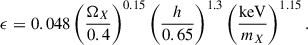
Here, ΩX is the density parameter of the dark matter. We consider three thermal WDM cosmologies, with particle mass corresponding to mX = 1 − 3 − 5 keV, respectively. Lighter models such as WDM1 and WDM3, with mX = 1 − 3 keV, have been ruled out by Lyman-α, number counts, UV luminosity function observations (Viel et al. 2013; Menci et al. 2016; Corasaniti et al. 2017; Dekker et al. 2022; Villasenor et al. 2023) and are used only for a broader characterization of WDM abundances and clustering. Furthermore, in WDM cosmologies, the halo mass function experiences a suppression given by (Lovell et al. 2014)
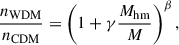 (3)
(3)
where γ = 2.7, β = −0.99 and Mhm is the half-mode mass, namely, the mass at which the transfer function in Eq. (1) is equal to 1/2.
We consider SIDM models with a constant cross section (SIDM1, with σ/mX = 1 cm2 g−1) and, more realistically, with the velocity-dependent cross section presented in Correa (2021, vSIDM), which rapidly declines at the typical velocity dispersion of massive bound systems. The model fits to observations of central densities of dwarf spheroidal galaxies, and it is based on a self-interaction described by a particle mass mX = 53.933 ± 9.815 GeV and a massive mediator in a Yukawa potential, with mass mφ = 6.605 ± 0.435 MeV (Correa 2021).
In Fig. 1 we show the spatial distribution of dark matter halos in box 50/B at different redshifts and cosmologies. The nodes and filaments become progressively clumpier toward low z, as they collect matter from the background. In particular, WDM models show a clear progressive suppression in the number density of bound structures. SIDM cosmologies, on the other hand, are not represented, since, upon qualitative inspection, they do not exhibit a significant difference with respect to ΛCDM.
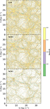 |
Fig. 1. From top to bottom: Spatial distribution of dark matter halos in box 50/B for the CDM, WDM3, and WDM1 cosmologies. The color bar shows the corresponding redshift in the range 0 < z < 2. |
3. The halo occupation distribution model
Discrete structures, such as galaxies and dark matter halos, arise at the overdensity peaks of the Universe; therefore, they are biased tracers of the underlying matter distribution. On large scales, this reduces to a linear, scale-independent relation between the halo and the dark matter density contrast fields, δh(x) and δ(x), through a bias factor, bh(z),
 (4)
(4)
On smaller scales, however, it is challenging to accurately model the clustering of halos because nonlinear effects emerge.
In recent years, the halo occupation distribution (HOD) formalism has been widely used in number count and clustering studies because it represents a simple and powerful theoretical tool for approximating galaxy abundances, bias, and small-scale galaxy clustering (Zheng et al. 2005; Giocoli et al. 2010; Asgari et al. 2023). It is based on the halo model, namely the idea that all the matter in the Universe is collected into halos (Cooray & Sheth 2002). Under this hypothesis, the question comes down to understanding how dark matter halos cluster together, based on their classification as central or satellites, and how luminous tracers, such as galaxies, correspondingly populate them.
3.1. Number counts
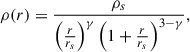
According to the HOD model, the average number of halos is given by
 (5)
(5)
where ⟨Nc⟩ is the average number of central halos, while ⟨Ns⟩ represents the average number of satellites. Unlike galaxy clustering, where ⟨Nc⟩ is parameterized according to the details of the galaxy formation process and of the uncertainties in the luminosity-mass relation, for dark matter halos it is simply given by a Heaviside step function (Zehavi et al. 2005),
 (6)
(6)
where Mmin is the mass cut of the sample, below which the number of central and satellite halos is equal to zero. There must be one central halo in order to have satellite halos, and thus, for masses higher than Mmin, where ⟨Nc⟩ = 1, we can write the number of subhalos as follows:
 (7)
(7)
where M1 and α are the normalization and slope of the power law, respectively, while the parameter M0 is included in more general HOD models, as a satellite truncation mass, which is different from Mmin. As we also find in our analysis, however, it is generally poorly constrained (Watson et al. 2009, 2012; Piscionere et al. 2015; Skibba et al. 2015).
In this sense, the halo occupation number, ⟨Nh⟩, gives us a first indication of the HOD parameters. Moreover, it allows us to test whether the distribution of satellites within halos of a given mass follows Poissonian statistics. In particular, we can investigate the average number of pairs associated with the same halo, which brings clustering information and is the base for the one-halo term of the two-point correlation function (Zheng et al. 2005),
 (8)
(8)
For a Poissonian distribution, this reduces to ⟨Nh(Nh − 1)⟩ = ⟨Ns⟩2 + 2⟨Ns⟩. Therefore, for massive halos that contain satellites, the ratio  , as we discuss in Sect. 4.1.
3.2. Radial distribution of subhalos
It is often assumed that the distribution of tracers follows the distribution of dark matter. For this reason, an NFW profile (Navarro et al. 1996) is generally adopted in clustering studies. However, it might not be sufficiently accurate to describe the small-scale distribution of subhalos, introducing systematic uncertainties in the parameter values of α and M1 and in cosmology. In particular, we expect the concentration of satellite halos, ch = fc c200c, to differ from that of dark matter, with fc as a free parameter of our model2. Therefore, following the approach of More et al. (2009), Watson et al. (2009, 2012) and Piscionere et al. (2015), we consider a generalized NFW (gNFW),
 (9)
(9)
where γ corrects the slope of the profile and rs = R200c/(fc c200c) is the scale radius, which varies depending on the halo mass and concentration. To estimate the latter, we use the c200c − M200c relation from Duffy et al. (2008). Finally, ρs = M200c/(4πrs3∫0R200c/fcx2 − γ/(1+x)3 − γdx) is the characteristic density, where x ≡ r/rs. For example, for a luminous red galaxy sample, the parameter γ is found to be an increasing function of luminosity, while fc is a decreasing one (Watson et al. 2012). We retrieve the NFW profile when both γ and fc are equal to one. A value of fc smaller than one boosts rs, eventually to a radius greater than R200c, which means that the density profile keeps its inner slope −γ even at larger radial separations, behaving like a pure power law (Watson et al. 2009, 2012). Therefore, in order to explore the full radial profile, the upper limit of the integral is adjusted accordingly. Differences in γ and fc among alternative cosmologies also account for variations of the profile shape and of the relative number of subhalos in the inner part of dark matter groups, respectively. As we show in the next section, this also impacts on the clustering properties of central and satellite halos.
3.3. Clustering
We use the HOD formalism to model the small-scale clustering of dark matter halos in cold and alternative dark matter scenarios. In particular, the halo model distinguishes two contributions to the correlation function,
 (10)
(10)
where ξ1h(r) is the one-halo term, accounting for the clustering of matter or tracers hosted by the same halo, while ξ2h(r) is the two-halo term, given by the pairs counted between different halos. The same formalism is equivalently written in Fourier space as
 (11)
(11)
In Eq. (11), the former term dominates at small scales, in a full nonlinear range, that is, below the typical size of dark matter halos, while the latter describes large-scale clustering, where the impact of nonlinearities is smaller and P(k) = bh2Plin(k). The linear power spectrum, Plin(k), is computed according to the approximation of Eisenstein & Hu (1998). This occurs for separations greater than the size of the largest dark matter halo.
Dealing with two different populations of tracers, in the one-halo term, we should separate the contribution of central-satellite and satellite-satellite pairs to the power spectrum, Pcs and Pss, respectively,
 (12)
(12)
In particular,
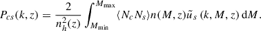 (13)
(13)
Here, the central and satellite occupation functions are independent, and therefore, ⟨NcNs⟩=⟨Nc⟩⟨Ns⟩. The normalized distribution of satellites within the halo, in Fourier space, is  , directly derived by numerically transforming Eq. (9), whose parameters are estimated by fitting the stacked satellite radial density profile measured in Sect. 4.2. This measurement is possible only with an adequate number of subhalos, which requires a group mass M200c > M1. In addition, halos of mass lower than M1 have R200c smaller than the minimum separation at which we measured the two-point correlation function in Sect. 4.3. From a physical point of view this is equivalent to exclude the one-halo contribution for groups with a central halo only.
For the halo mass function, n(M, z), we adopt the functional form provided by Tinker et al. (2008). It can be integrated to compute the total halo number density,
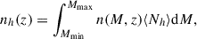 (14)
(14)
in which ⟨Nh⟩ is expressed through Eq. (5). The satellite-satellite power spectrum is
 (15)
(15)
Finally, the two-halo power spectrum is given by
![Mathematical equation: $$ \begin{aligned} P_{2h}(k, z)&= P_\mathrm{lin} (k, z) \Bigg [\frac{1}{n_h(z)} \int _{M_{\min }}^{M_{\max }} \langle N_{h}\rangle n(M, z) b(M, z)\nonumber \\&\quad \times \tilde{u}_s(k, M, z) \, \mathrm{d} M \Bigg ]^2 (A+Bk+Ck^2), \end{aligned} $$](/articles/aa/full_html/2026/03/aa58242-25/aa58242-25-eq18.gif) (16)
(16)
where b(M, z) is the linear bias provided by Tinker et al. (2010), while A, B and C form a scale-dependent nonlinear correction (see for example Smith et al. 2007), which reproduces the small-scale two-halo clustering of groups. Indeed, a more accurate description of the transition region where the one-halo and the two-halo contributions are almost equivalent, called quasi-linear regime, is traditionally more difficult to model (Mead et al. 2015), and requires to consider nonlinear bias (van den Bosch et al. 2013; Bhowmick et al. 2018) and exclusion effects (Tinker et al. 2005). Discrete tracers, such as galaxies and dark matter halos, cannot overlap; thus the distance r among them is always larger than the sum of their radii (Baldauf et al. 2013). This reduces the two-halo correlation function at small scales. Moreover, the two-halo term itself has a small-scale behavior that cannot be reproduced by the assumption of the model bias presented in Tinker et al. (2010), as it contains nonlinearities that, if not taken into account, would alter the two-point correlation function at the typical one-halo separation, ending up with systematic errors on the HOD parameters. Moreover, the impact of exclusion effects is limited by the abundance of groups with mass between 108 M⊙ h−1 and 1010 M⊙ h−1, which have R200c < 0.05 Mpc h−1. This also allows us to count the two-halo pairs with spatial separations that are fully in the nonlinear regime. For this reason, for each redshift and cosmological model, we calibrate the nonlinear deviation from bh2Plin(k, z), summarized in the parameters A, B and C, by modeling the clustering of dark matter groups only, without considering the contribution of satellites.
On large scales, the shape of the correlation function is determined by ⟨Nh⟩, and essentially differs from the matter-matter correlation for a linear bias factor only. On the other hand, on small scales, the one-halo term is sensitive to ⟨Nh(Nh − 1)⟩ (Berlind & Weinberg 2002). A higher slope value, α or a lower normalization M1, determines an increase in the number of satellites at high M. This largely boosts the number of satellite-satellite pairs in the one-halo term of the two-point correlation function. It also impacts the two-halo term, since higher masses, which are strongly biased, become more populated. In other words, for a given number of halos, we remove substructures from low-mass systems, redistributing them into more massive ones. Furthermore, higher values for γ and fc, as in Eq. (9), steepen the satellite density profile, increasing the amplitude and the slope of the one-halo correlation function.
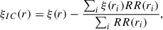
In Fig. 2 we show the different contributions to the two-point correlation function as a function of redshift, for a CDM cosmology and M > 108 M⊙ h−1. In particular, on large scales, ξ2h(r) is largely suppressed by the finite size of the box. This condition is called ‘integral constraint’ and requires to be forward-modeled in order to obtain unbiased results, as discussed in Sect. 4.3. On the other hand, on small scales, the predictions of the linear model are not accurate enough. In particular, at high redshift, the scale-dependent terms, B and C, are more relevant, while at z = 0 the constant A deviates more from 1. For example, at z = 2 we found A = 0.80 ± 0.04, B = 0.41 ± 0.02 and C = −0.010 ± 0.002, while at z = 0, A = 0.67 ± 0.03, B = 0.07 ± 0.01 and C = −0.004 ± 0.001. Although ξ1h(r) always overcomes the linear ξ2h(r) at r < 0.2 Mpc h−1, it prevails on the nonlinear two-halo term only at z = 0. It is dominated by satellite-satellite pairs, meaning that our dark matter groups are largely populated by subhalos. On the other hand, the correlation function of the central-satellite pairs, ξcs, increases with the redshift in absolute terms and relative to its satellite-satellite counterpart, ξss. Their ratio extends from a maximum of approximately 0.09 at z = 0 to 0.36 at z = 2. Given the same mass cut of 108 M⊙ h−1, moving toward high z, we find a larger contribution of isolated or poorly populated halos. Conversely, when we only select subhalos with a mass greater than 109 M⊙ h−1, the term ξcs becomes progressively more important and dominates ξss for M > 1010 M⊙ h−1.
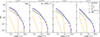 |
Fig. 2. From left to right: Different contributions to the two-point correlation function from z = 0 to z = 2. The blue circles represent the measurement for box 50/A for CDM cosmology considering halos with M > 108 M⊙ h−1. The corresponding errors are obtained with the jackknife method. The one-halo term is given by the dotted purple line and it is the sum of ξcs (solid orange line) and ξss (solid yellow line). The linear two-halo term (cyan dashed line) is then corrected for integral constraint, nonlinearities and halo exclusion (dashed red line). Finally, the solid black line represents the total best-fit model. |
4. Results
In this section, we present the main results of our study on the halo occupation function, the subhalo distribution, and clustering. We discuss the outcome of the measurements in the CDM and alternative dark matter scenarios, and we then focus on our constraints on the HOD and density profile parameters. The Bayesian analysis was performed by adopting a Gaussian likelihood for each redshift bin
 (17)
(17)
where mi is the model on the radial scale ri, di is the measurement, and σi is the associated error.
4.1. Number counts
For each FOF group in the box at redshift z, the AIDA-TNG project gives access to the mass M200c. Around each halo position, (xh, yh, zh), we build a sphere of comoving radius R200ccom and count the number of subhalos within the region. Then, we split the group catalog by averaging the counts into ten logarithmic mass bins. In the same way, we also measured ⟨Nh(Nh − 1)⟩.
Fig. 3 clearly separates the contribution of the central halo from that given by the associated substructures, namely the satellite halos. The applied mass selection ensures that there is at least one halo for M200c > Mmin, while subhalos are counted from M200c > M1. In the top panels we show the average number of pairs, ⟨Nh(Nh − 1)⟩. As explained in Sect. 3.1, this quantity enables us to determine whether the subhalo population follows a Poissonian distribution. Although the differences between cosmologies are negligible, we observe that the hypothesis is fully satisfied when M200c > M1, where the number of satellites begins to deviate from zero.
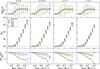 |
Fig. 3. From left to right: Average number of dark matter pairs (top panels), halo occupation function (middle panels) and residuals (bottom panels) with respect to the CDM reference level (solid blue line) as a function of M200c in box 50/A in the range 0 < z < 2 for CDM (blue circles), WDM3 (black triangles), WDM5 (crimson diamonds), SIDM1 (gold pentagons), and vSIDM (green triangles). The corresponding errors are computed with the standard deviation of the measurements for each mass bin. The dashed horizontal gray line represents the expected ratio for a Poissonian distribution. The solid horizontal gray line marks the central halo that always exists for M200c > Mmin. |
In Fig. 3 we also show the occupation function ⟨Nh⟩ for each dark matter model. Alternatives to CDM are characterized by a reduction in the average number of satellites, with larger departures for the more massive systems. In WDM scenarios, this is particularly pronounced. For WDM3, the comparison with CDM shows residuals that exceed -0.5 for M200c > 1011 M⊙ h−1. A different mass selection, namely Mmin > 109 M⊙ h−1, significantly attenuates the effect, clarifying its strong dependence on the mass as a consequence of free streaming. For such a mass cut, only the warmest model, namely WDM1, exhibits a difference with respect to WDM3 and CDM, as we show in Fig. 4. Here, we fit Eq. (5) to quantify the dependence of α and M1 on the redshift and mass selection of our sample; M0, which represents only an offset in the mass of the group in the numerator, is not constrained and its presence does not significantly modify the mean values of α and M1, although it widens their posterior distributions. For the sake of example, in Fig. 4 we show some results for boxes 50/A and 50/B. In particular, we note that for Mmin > 108 M⊙ h−1, we have ![Mathematical equation: $ \log[{M_1}/({\mathrm{M}_\odot\,h^{-1}})]=10.42^{+0.25}_{-0.18} $](/articles/aa/full_html/2026/03/aa58242-25/aa58242-25-eq20.gif) at z = 0 and
at z = 0 and ![Mathematical equation: $ \log[{M_1}/({\mathrm{M}_\odot\,h^{-1}})]=10.24^{+0.20}_{-0.16} $](/articles/aa/full_html/2026/03/aa58242-25/aa58242-25-eq21.gif) at z = 2, reflecting the fact that despite the presence of more massive structures, the average number of satellites in a given mass bin is slightly reduced in the local Universe by tidal disruption and merging phenomena. In fact, due to the hierarchical growth of cosmic structures, we first expect the formation of low-mass halos, which represent the progenitors of the systems that we count at z = 0, which can host more than 103 subhalos. In contrast,
at z = 2, reflecting the fact that despite the presence of more massive structures, the average number of satellites in a given mass bin is slightly reduced in the local Universe by tidal disruption and merging phenomena. In fact, due to the hierarchical growth of cosmic structures, we first expect the formation of low-mass halos, which represent the progenitors of the systems that we count at z = 0, which can host more than 103 subhalos. In contrast,  at z = 0 and
  at z = 2, which means that ⟨Nh⟩ increases approximately with the same slope at different redshifts.
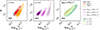 |
Fig. 4. Posterior distributions of the halo occupation function, ⟨Nh⟩, for different dark matter cosmologies (left panel), mass selections (middle panel), and redshifts (right panel). Different dark matter models are tested in box 50/B, with a mass selection of Mmin > 109 M⊙ h−1. The other two panels consider the CDM cosmology in box 50/A. |
As also shown in Fig. 4, a higher minimum mass tends to significantly increase the value of the normalization, while the slope rises only slightly. At z = 0, for Mmin > 109 M⊙ h−1 we have ![Mathematical equation: $ \log[{M_1}/({\mathrm{M}_\odot\,h^{-1}})]=11.47^{+0.23}_{-0.16} $](/articles/aa/full_html/2026/03/aa58242-25/aa58242-25-eq24.gif) and
and  , while for Mmin > 1010 M⊙ h−1 we have
 ![Mathematical equation: $ \log[{M_1}/({\mathrm{M}_\odot\,h^{-1}})]=12.25^{+0.20}_{-0.17} $](/articles/aa/full_html/2026/03/aa58242-25/aa58242-25-eq26.gif) and
and  , indicating that more massive halos tend to have relatively more massive substructures (Zehavi et al. 2005). Finally, the broadening of the posterior distribution is a consequence of the lower statistics.
Since in SIDM models the number density of dark matter halos does not differ significantly from the CDM case, as shown in Despali et al. (2025), the reduction in the average number of subhalos can be interpreted as a consequence of the more diffuse central density peak in self-interacting models, which results in satellite density profiles which are in general shallower around the core. In other words, moving toward outer regions, for a given mass, the cumulative radial count of subhalos presents a slope higher than the corresponding CDM model. However, these differences only result in a minimal increase and decrease in M1 and α, respectively, which, however are not sufficient to discriminate between dark matter models.
4.2. Radial distribution of subhalos
In order to disentangle the contribution of the central and satellites to the clustering signal of dark matter halos, we need to study how satellites are distributed within their hosts. To do this, we split the halos into ten logarithmic-spaced mass bins, with a lower limit given by the transition mass from the central-dominated to the satellite-dominated regime of Fig. 3, at z = 0, which depends on the resolution of the boxes, and corresponds to 1010 M⊙ h−1 for 50/A. For each mass bin, we consider Nbin = 8 logarithmic-spaced radial bins. In practice, from the middle value of each mass bin we estimate the corresponding comoving radius R200ccom, which is adopted as Rmax, while Rmin = Rmax/(Nbin − 1), to exclude the innermost regions, where there is a lack of satellites due to mass selection, tidal disruption, and resolution effects. The counts are then averaged for every mass bin, and normalized according to the comoving volume of the i−th radial shell,  , obtaining
  , our stacked profile.
From measurements of the radial subhalo distribution, we can quantify possible deviations from a pure NFW model. Dealing with discrete tracers rather than a continuous dark matter density field, we compute the characteristic number density of satellites as
 (18)
(18)
where M200c corresponds to the average in a given mass bin, ρ(r) is given by Eq. (9), and
 (19)
(19)
is the normalization factor measured from the radial density profile,  .
.
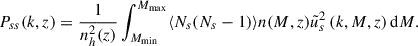
Figure 5 shows the radial distribution of subhalos normalized to the average value of the satellite density at a radius of R200c, for standard ΛCDM and the alternative dark matter models. Variations among different masses are highlighted, while for r > 0.5 × R200c the rescaled radial profiles are relatively self-similar; a feature that, however, is lost at higher redshifts because of the selection effects, which impact more when the average mass of structures is lower. In general, more massive structures are denser in terms of the number of satellites. This is because the effect of dynamical friction is progressively more relevant for massive subhalos hosted by large dark matter groups. As a consequence, they sink toward the halo center, reducing the radius of their orbits and enhancing the inner part of the density profile, while the outer region is less affected (Han et al. 2016; Chang et al. 2018). This fact incidentally explains why luminous galaxies are poor tracers of the NFW dark matter density distribution, while they match the corresponding subhalo profiles found in cosmological simulations (Watson et al. 2012; Chang et al. 2018). Conversely, since the halo mass is inversely correlated with the age, smaller hosts at z = 0 are, on average, older and have had more time to destroy subhalos located near the center. Interestingly, the situation is reversed in SIDM1 model, for which low-mass groups, with log[M200c/(M⊙ h−1)] of 10.7 and 11.2 are centrally more peaked than the massive ones, with log[M200c/(M⊙ h−1)] of 12.6 and 13.1, which have thermalized earlier. In fact, self-interaction between dark matter particles produces more diffuse central peaks and more extended cores for high-mass halos (Despali et al. 2025). While in vSIDM scenario the cross-section is a decreasing function of the relative velocity of particles, in SIDM1 it is constant. Therefore, moving toward the typical galaxy cluster size, this scenario is strongly constrained (Meneghetti et al. 2001; Eckert et al. 2022; Shen et al. 2022) since it could cause major departures from the ΛCDM cosmology; these are, however, ruled out by observations that found cusps at the center of galaxy clusters (Newman et al. 2013).
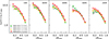 |
Fig. 5. From left to right: Radial distribution of dark matter subhalos at z = 0 for various mass bins and dark matter models. The triangles represent bins with a group mass of log[M200c/(M⊙ h−1)] = 10.7 (green), 11.2 (gray), 12.6 (gold), and 13.1 (red), respectively. The solid, colored lines reflect the gNFW best-fit model. The corresponding errors are computed with the standard deviation of the measurements, for each mass bin. |
In Fig. 5 we show the best fit, calculated according to Eq. (18). In addition to gNFW, we also test the density profile model presented in Einasto (1965). Although it performs well if we analyze the full density profile up to scales larger than R200c, it fails at small separations and for low mass halos, for which the friction force is not enough to flatten the spatial distribution of satellites within the core. We estimate the parameters of the gNFW profile, γ and fc, choosing large, flat priors, between [ − 10, 2] and [0.1, 1.5], respectively. In Fig. 6, for a ΛCDM cosmology, we show the mass and redshift evolution of the density profile parameters, considering only mass bins where halos are present at all redshifts and for all cosmologies. In particular, γ assumes negative values, reflecting the well-established results that the halo distribution is antibiased (Ghigna et al. 1998; Springel et al. 2008), namely it is more cored toward the center than the matter density. The analytical model presented in Han et al. (2016) explains the spatial distribution of subhalos as a result of tidal stripping, generated from dynamical friction which, conversely, does not affect the dynamics of dark matter particles. Furthermore, γ increases with the mass of the group M200c, which means that less massive systems generally present a shallower radial distribution of satellites. However, we should consider that a variation in M200c from approximately 1013 M⊙ h−1 to 1010 M⊙ h−1 translates into a reduction of R200c of about one order of magnitude; therefore we explore a shorter range of spatial separations in low-mass groups. In this case, the value of γ reflects the lack of subhalos toward more central regions, due to stripping phenomena, box resolution and selection effects. Also for this reason, the majority of subhalos are located in the outer regions of the group, which correspond to shells of larger volume.
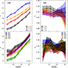 |
Fig. 6. Marginalized posterior distribution of the gNFW parameters, γ (left) and fc (right), for different mass bins. Top panels: Evolution with redshift for a fixed ΛCDM cosmology. Bottom panels: Evolution in alternative dark matter models at z = 0. The errors represent the 68% percentiles. |
In high-z Universe, dark matter subhalos form in an environment with a higher mean matter density, which allows a more efficient accretion process. In addiction, they are less massive and more concentrated. These features translate into a reduction of the tidal stripping. Furthermore, over time, their average number decreases as they merge. Having measured the density in comoving radial shells, only the net effect of satellite creation and destruction is considered, while the total mass of the central peak increases toward z = 0. Thus, in time the satellite density profiles become flatter. This explains the redshift evolution of the γ − M200c relation that we see in Fig. 6. On the other hand, the concentration factor, fc, is roughly constant for halos in a wide range of masses and redshift, which share the same deviation from the adopted c − M200c relation. This simply describes a general shrinking in the characteristic radius rs with respect to that of the dark matter density profile, reflecting the loss of orbital energy of the subhalos that experience dynamical friction (Chang et al. 2018).
In Fig. 6 we also see the variation of the gNFW density profile parameters in the different dark matter scenarios. Although the general mass and redshift tendencies are kept, there is no clear dependence of fc on cosmology. Instead, WDM models prefer a higher γ, which means that the subhalos radial distribution is more concentrated and steeper around the center, as also found in the analysis of the Aquarius-WDM runs (Lovell et al. 2014), the COCO simulations (Bose et al. 2017) and zoom-in simulations of early type galaxies from the EAGLE box (Despali et al. 2020). Indeed, the free-streaming of dark matter particles determines an overall delay in the structure formation process, especially for less massive systems (Lovell 2024). Therefore, WDM subhalos of a given mass generally form later than their CDM counterparts, when the average density of the Universe is smaller, allowing more concentrated structures to grow. Conversely, in SIDM scenarios, γ is generally lower, which means that the innermost satellite density profile is shallower and less concentrated. This result has been already found in simulations by Fischer et al. (2022, 2024), as a reduction in the number of subhalos becoming progressively stronger at smaller distances to the host, and can be interpreted as a consequence of core thermalization due to particle interaction. This is in fact expected to produce a flatter underlying dark matter distribution and make satellites more sensitive to tidal disruption. For this reason, the relative number of subhalos is distributed toward the external radial shells of the FOF group. At z = 0, for M200c > 1012.5 M⊙ h−1, the radial distribution of the SIDM1 subhalos becomes shallower than that of the vSIDM. This once again highlights the tendency of SIDM1 to form cores even in the most massive systems, while vSIDM interactions are only significant for low-mass bound structures. The behavior of WDM and SIDM cosmologies, quantitatively appreciable already in Fig. 5, is also reflected in their clustering properties, as explained in Sect. 4.3.
4.3. The two-point correlation function
The clustering information of a sample of discrete tracers is encoded in the two-point correlation function, ξ(r). According to the definition, for a pair of elements located in volume elements δV1 and δV2, at a given separation r, it is expressed as an excess probability with respect to a uniform distribution,
![Mathematical equation: $$ \begin{aligned} \delta P_{12}(r) = n_V^2\,[1+\xi (r)]\,\delta V_1 \delta V_2, \end{aligned} $$](/articles/aa/full_html/2026/03/aa58242-25/aa58242-25-eq33.gif) (20)
(20)
where nV is the mean tracer number density in a unit of comoving volume.
We build the random catalog by uniformly extracting the comoving coordinates of dark matter halos in a box. Since for each redshift the number of tracers is higher than 4 × 10⁵, the shot noise is limited, and the size of the random catalog is kept equal to the size of the original one, in order to speed up the computation. We measure the real-space two-point correlation function with the Landy & Szalay (1993) estimator,
 (21)
(21)
which provides an unbiased measurement of ξobs(r) once the normalized number of data-data, random-random, and data-random pairs, DD(r), RR(r) and DR(r) respectively, is counted. The errors are estimated using the jackknife method, considering a number of regions equal to 125 (Norberg et al. 2009). We adopt appropriate mass cuts to ensure completeness, corresponding to a lower limit of 108 M⊙ h−1 for 50/A. The two-point correlation is measured into fifteen logarithmic-spaced bins between 0.05 Mpc h−1 and 15 Mpc h−1. The lower limit is motivated by the resolution of the simulation, whereas the upper limit is due to the finite size of the box and corresponds approximately to the scale at which the correlation function becomes negative. At these scales nonlinear effects are not negligible and the halo bias depends on r, as well as on redshift and mass. A higher-mass cut selects only more massive halos, which are more biased, and therefore provides a stronger clustering signal. Furthermore, with cosmic time, the one-halo term becomes more pronounced, implying a progressive increase of nonlinearities.
The use of cosmological simulations with size much smaller than the volume of the Universe has non-negligible consequences on the measurement of the clustering signal. From a theoretical point of view, a scale-free power spectrum satisfies the condition P(k = 0) = 0, which corresponds to imposing homogeneity of matter fluctuations on sufficiently large scales, where the cosmological principle is satisfied (Riquelme et al. 2023). According to the definition of probability, the integral of Eq. (20) over the full volume of the Universe is equal to 1. The same condition also holds if we consider the finite volume of the box, Vb. This implies that
 (22)
(22)
which means that we should find a scale at which ξobs(r) becomes negative, which is lower than the corresponding scale for the model of ξ(r). In other words, the evaluation of the correlation function in a limited volume determines a reduction in the clustering signal. The observed correlation function is linked to the theoretical one through a window function, W(r). In Eq. (22), in order to avoid volume integration in surveys with complicated geometries, it is common to correct the model prediction by following the radial evolution of random-random pairs. This information is contained in the shape of the random catalog. Such ‘integral constraint’ condition therefore takes the form (Ross et al. 2013; Riquelme et al. 2023)
 (23)
(23)
and spans over the range at which the pairs are counted.
In Fig. 7, we compare the measures obtained in box 50/A within the ΛCDM framework, with the results in alternative dark matter scenarios, finding that the main difference between models is located at the one-halo scales, corresponding to r ≲ 1 Mpc h−1. In fact, SIDM1 and vSIDM are systematically less clustered, and the difference to CDM is only slightly affected by time evolution, since they residuals remain between −5 and −2.5 for all the redshifts considered. In particular, it is noteworthy that SIDM1 is closer to CDM at high z, indicating a late-time thermalization of the core; conversely, the vSIDM model deviates more at z = 2. In other words, vSIDM is more effective at high z, since the cross-section is higher for low-mass halos, where the velocity dispersion of the particles is smaller. On the other hand, in WDM cosmologies, the average delay in the structure formation process makes clustering differences more visible at high z, with residuals larger than 2.5 for r ≲ 1 Mpc h−1 and r ≲ 0.2 Mpc h−1, for WDM3 and WDM5, respectively. These results reinforce what we already found from the analysis of Sect. 4.2, according to which WDM generally produces a more peaked subhalo density distribution. As we have already seen in Sect. 3.3 the satellite-satellite pairs dominate the one-halo range. Consequently, the radial distribution of the satellites directly affects the clustering properties of the full halo population. However, the excess of clustering is also found in the two-halo term for the warmest models. Again, we can interpret this trend as a consequence of free-streaming of the particles. Indeed, the suppression of low-mass dark matter halos has a direct impact on the halo mass function, which operates as a weighting factor for the halo bias, resulting in practice in a larger effective bias of our sample.
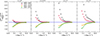 |
Fig. 7. From left to right: Residuals of the two-point correlation function for alternative dark matter models for redshifts from z = 0 to z = 2. The blue, horizontal line represents the reference level for ΛCDM model. WDM3 (black triangles), WDM5 (crimson diamonds), SIDM1 (gold pentagons) and vSIDM (green triangles) are also shown. |
A proper modeling of the observed two-point correlation function is well beyond the linear theory, requiring a generalization of the density profiles and the introduction of the HOD formalism. Our ultimate goal is to explore the degeneracy of HOD parameters in different cosmological frameworks. For this reason, as already described in Sect. 3.3, we calibrate the nonlinear deviation from bh2Plin(k, z), by modeling the clustering of dark matter groups only, without considering the contribution of satellites. In this way, we quantify the A + Bk + Ck2 factor of Eq. (16), which incorporates the exclusion effects and the inaccuracies of the nonlinear bias model for each redshift and dark matter scenario, adopting their median value for the HOD characterization of the full halo populations.
Then we fit Eq. (10) to constrain the parameters M1 and α, whose posterior distributions are not affected by the presence of M0. We set the latter to zero, to reduce the number of parameters and thus the complexity of the model. In order to assume a physically motivated normalized density profile,  , we adopt flat priors on the parameters fc and γ, according to the range permitted by the posterior distributions presented in Sect. 4.2, while log[M1/(M⊙ h−1)] and α are left free to vary in the range [9, 13] and [0.7, 1.6], respectively. For the WDM models, we use Eq. (1) to suppress the linear power spectrum, Plin(k, z), at small scales, while for the halo mass function, n(M), we apply Eq. (3). This reduces the low-mass halo population, resulting in a higher effective bias, which determines an enhancement of the two-halo term. SIDM models, on the other hand, share the same power spectrum and mass function as ΛCDM.
In Fig. 8 we show the marginalized posterior distribution in the M1 − α plane. The constraints on HOD parameters are in agreement with the results obtained in Sect. 4.1 with halo occupation function. In particular, for the ΛCDM cosmology, we find ![Mathematical equation: $ \log[{M_1}/({\mathrm{M}_\odot\,h^{-1}})]=10.41^{+0.15}_{-0.12} $](/articles/aa/full_html/2026/03/aa58242-25/aa58242-25-eq38.gif) and
and  at z = 0;
 ![Mathematical equation: $ \log[{M_1}/({\mathrm{M}_\odot\,h^{-1}})]=9.93^{+0.09}_{-0.09} $](/articles/aa/full_html/2026/03/aa58242-25/aa58242-25-eq40.gif) and
and  at z = 2. However, they are also more competitive. In fact, the two-halo term of the correlation function relies on ⟨Nh⟩, as in the case of number counts, while the one-halo term depends on the number of pairs ⟨Nh(Nh − 1)⟩. In addition to second-order statistics, the clustering model also includes stringent prior information from the parameters of the gNFW density profile, fc and γ. This emphasizes the necessary synergy between these different probes for future HOD-based studies.
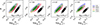 |
Fig. 8. Marginalized posterior distributions of the HOD parameters in the M1 − α plane for box 50/A and M > 108 M⊙ h−1. The 68% and 95% contours are represented for CDM (blue), WDM3 (black), WDM5 (crimson), SIDM1 (gold) and vSIDM (green) cosmological models. |
Clustering of halos reveals its full potential when applied to alternative dark matter scenarios. The M1 parameter indeed increases in the WDM and SIDM models, alongside a slight decrease in α. This reflects the fact that the average reduction in the number of satellites due to free streaming or core thermalization means that higher group masses are required for finding the same number of subhalos. This tendency was already observed in Sect. 4.1, where we analyzed the occupation functions; however, the ability to distinguish between different models was limited to box 50/B, for which only WDM1 presented a 1σ difference with CDM, for the parameter M1. From this point of view, the study of the two-point correlation function represents a powerful probe, especially if we analyze the clustering of dark matter halos at high z. In particular, for the thermal WDM3 model we find ![Mathematical equation: $ \log[{M_1}/({\mathrm{M}_\odot\,h^{-1}})]=10.83^{+0.11}_{-0.11} $](/articles/aa/full_html/2026/03/aa58242-25/aa58242-25-eq42.gif) and
and  at z = 0;
 ![Mathematical equation: $ \log[{M_1}/({\mathrm{M}_\odot\,h^{-1}})]=10.16^{+0.07}_{-0.06} $](/articles/aa/full_html/2026/03/aa58242-25/aa58242-25-eq44.gif) and
and  at z = 2. In other words, the normalization in the number of satellites exhibits a difference greater than 2σ with respect to CDM, while at z = 2, the one on the slope is at the level of 1σ. WDM5 occupies an intermediate position, with
 ![Mathematical equation: $ \log[{M_1}/({\mathrm{M}_\odot\,h^{-1}})]=10.53^{+0.13}_{-0.11} $](/articles/aa/full_html/2026/03/aa58242-25/aa58242-25-eq46.gif) and
and  at z = 0;
 ![Mathematical equation: $ \log[{M_1}/({\mathrm{M}_\odot\,h^{-1}})]=9.95^{+0.08}_{-0.08} $](/articles/aa/full_html/2026/03/aa58242-25/aa58242-25-eq48.gif) and
and  at z = 2, and therefore requires more stringent mass cuts to achieve the same level of disagreement. Inspecting Fig. 8, it is also clear that fixed and velocity-dependent SIDM models are indistinguishable from each other. As the latter acts mainly where the velocity dispersion of the particles is lower, altering the structure and distribution of small-mass halos, we conclude that simulations with higher mass resolution are required to explore finer spatial scales in detail and to better highlight the differences between alternative dark matter models. In the future, we plan to exploit the full-physics AIDA-TNG simulations, for a subsequent work, which will take into account the fact that not all dark matter halos and subhalos are able to host galaxies, as well as the complicated relationship between the mass and the luminosity of galaxies, directly linked to their formation processes. In this way, with more complete HOD models, we aim at disentangling the effects of alternative dark matter from baryonic physics, in preparation for a full comparison with observational data from galaxy clustering.
5. Conclusions
We studied the effect of warm and self-interacting dark matter models on the abundance, the radial distribution, and the clustering properties of subhalos. For this purpose, we used a set of dark matter-only cosmological boxes with a variable size and resolution that were developed within the AIDA-TNG project. We applied the HOD formalism, which allowed us to separate the contributions of distinct populations of central and satellite halos, in order to model their occupation function and clustering. In particular, we counted the average abundances of subhalos within the comoving radius R200ccom for different mass bins and found that the HOD parameter M1 is higher at low redshift as a consequence of the impact of tidal stripping and merging phenomena on the average number of satellites. Alternative dark matter cosmologies predict a reduction in the number of subhalos within R200ccom. In WDM models, particle free streaming indeed suppresses the formation of low-mass halos, while in the SIDM case, the core thermalization redistributes satellites in the outer region of dark matter groups. However, while for box 50/B for M > 109 M⊙ h−1, CDM and WDM1 cosmologies exhibit an appreciable difference, in box 50/A for M > 108 M⊙ h−1, the occupation function does not provide a significant way to distinguish between models, requiring higher statistics and/or mass resolution. Moreover, with the applied mass selections, we verified that for the group mass M200c > M1, where the average number of satellites is larger than one, they follow a Poissonian distribution for all the models considered.
We also evaluated the radial distribution of subhalos around the centers of the groups. To do this, we counted the average number density of satellites in spherical shells up to a radius equal to R200ccom. For each mass bin and dark matter model, we fit the stacked radial density with a gNFW density profile. In this way, we were able to constrain the evolution of the gNFW parameters γ and fc with M200c and z. Although the latter is approximately constant and larger than one, as a consequence of dynamical friction, we found that the subhalo distribution becomes steeper for more massive systems at high-z, while it remains antibiased compared to the matter distribution. Furthermore, SIDM models generally prefer a shallower satellite radial profile as a result of the core thermalization in bounded dark matter halos, while WDM cosmologies on average admit a more cusped distribution toward the center of the groups as a result of the delayed structure formation process. This has direct consequences on the clustering properties of dark matter halos because it mainly affects the one-halo term of the two-point correlation function, where the differences between cold and alternative dark matter models are more relevant. In particular, in WDM cosmologies, the peaked subhalo distribution determines a clustering excess at r ≲ 0.2 Mpc h−1, with an increasing effect toward high z. At z = 2, it indeed also extends to the two-halo scales; the free streaming of dark matter particles determines a low-mass suppression in the halo mass function, which increases the effective bias of our sample. Conversely, SIDM models are less clustered at small scales, and their residuals with respect to CDM are only slightly affected by the redshift evolution. The HOD modeling of the two-point correlation function provided constraints on M1 and α that agree with the prediction of the halo occupation functions. In addition, it produced more stringent results, with a 2σ difference on M1 between CDM and WDM3 from z = 0 to z = 2. This revealed the effectiveness of this cosmological probe in distinguishing between possible alternative dark matter scenarios.
In the future, we plan to conduct a study on full-physics simulations to explore the degeneracy between the properties of dark matter particles and the physics of baryons in macroscopic observables, such as abundances, density profiles, and clustering. Variations in the physics of dark matter modify the abundance and the spatial distribution of halos, with a possible direct and macroscopic impact on luminous tracers, such as galaxies. Therefore, the completeness, spatial resolution, and depth of forthcoming photometric and spectroscopic surveys, combined with new state-of-the-art simulations, will offer unique possibilities to shed light on the real nature of dark matter.
Acknowledgments
We thank Ravi Sheth for useful discussions and hints on the paper. We would like to thank the anonymous referee for the constructive comments, which have improved the quality of the manuscript. We acknowledge the financial contribution from the grant PRIN-MUR 2022 20227RNLY3 “The concordance cosmological model: stress-tests with galaxy clusters” supported by Next Generation EU and from the grants ASI n.2018-23-HH.0 and n. 2024-10-HH.0 “Attivitá scientifiche per la missione Euclid – fase E”, and the use of computational resources from the parallel computing cluster of the Open Physics Hub (https://site.unibo.it/openphysicshub/en) at the Physics and Astronomy Department in Bologna. GD acknowledges the funding by the European Union - NextGenerationEU, in the framework of the HPC project – “National Centre for HPC, Big Data and Quantum Computing” (PNRR – M4C2 – I1.4 – CN00000013 – CUP J33C22001170001). We acknowledge ISCRA and ICSC for awarding this project access to the LEONARDO supercomputer. The AIDA-TNG simulations where run on the LUMI supercomputer (Finland), thanks to the award of computing time through a EuroHPC Extreme Scale Access call.
References
- Abbott, T. M. C., Aguena, M., Alarcon, A., et al. 2022, Phys. Rev. D, 105, 023520 [CrossRef] [Google Scholar]
- Adhikari, S., Banerjee, A., Boddy, K. K., et al. 2025, Rev. Mod. Phys., 97, 045004 [Google Scholar]
- Amon, A., Gruen, D., Troxel, M. A., et al. 2022, Phys. Rev. D, 105, 023514 [NASA ADS] [CrossRef] [Google Scholar]
- Asgari, M., Lin, C.-A., Joachimi, B., et al. 2021, A&A, 645, A104 [NASA ADS] [CrossRef] [EDP Sciences] [Google Scholar]
- Asgari, M., Mead, A. J., & Heymans, C. 2023, Open J. Astrophys., 6, 39 [NASA ADS] [CrossRef] [Google Scholar]
- Baldauf, T., Seljak, U., Smith, R. E., Hamaus, N., & Desjacques, V. 2013, Phys. Rev. D, 88, 083507 [NASA ADS] [CrossRef] [Google Scholar]
- Bardeen, J. M., Bond, J. R., Kaiser, N., & Szalay, A. S. 1986, ApJ, 304, 15 [Google Scholar]
- Berlind, A. A., & Weinberg, D. H. 2002, ApJ, 575, 587 [Google Scholar]
- Bhowmick, A. K., Di Matteo, T., Feng, Y., & Lanusse, F. 2018, MNRAS, 474, 5393 [Google Scholar]
- Bode, P., Ostriker, J. P., & Turok, N. 2001, ApJ, 556, 93 [Google Scholar]
- Bose, S., Hellwing, W. A., Frenk, C. S., et al. 2017, MNRAS, 464, 4520 [Google Scholar]
- Bower, R. G., Benson, A. J., Malbon, R., et al. 2006, MNRAS, 370, 645 [Google Scholar]
- Boylan-Kolchin, M., Bullock, J. S., Kaplinghat, M., et al. 2011, MNRAS, 415, L40 [NASA ADS] [CrossRef] [Google Scholar]
- Brooks, A. M., Kuhlen, M., Zolotov, A., & Hooper, D. 2013, ApJ, 765, 22 [NASA ADS] [CrossRef] [Google Scholar]
- Bullock, J. S., & Boylan-Kolchin, M. 2017, ARA&A, 55, 343 [Google Scholar]
- Busha, M. T., Alvarez, M. A., Wechsler, R. H., Abel, T., & Strigari, L. E. 2010, ApJ, 710, 408 [Google Scholar]
- Carucci, I. P., & Corasaniti, P.-S. 2019, Phys. Rev. D, 99, 023518 [NASA ADS] [CrossRef] [Google Scholar]
- Castellano, M., Yue, B., Ferrara, A., et al. 2016, ApJ, 823, L40 [NASA ADS] [CrossRef] [Google Scholar]
- Chang, C., Baxter, E., Jain, B., et al. 2018, ApJ, 864, 83 [NASA ADS] [CrossRef] [Google Scholar]
- Chisari, N. E., Richardson, M. L. A., Devriendt, J., et al. 2018, MNRAS, 480, 3962 [Google Scholar]
- Cooray, A., & Sheth, R. 2002, Phys. Rep., 372, 1 [Google Scholar]
- Corasaniti, P. S., Agarwal, S., Marsh, D. J. E., & Das, S. 2017, Phys. Rev. D, 95, 083512 [NASA ADS] [CrossRef] [Google Scholar]
- Correa, C. A. 2021, MNRAS, 503, 920 [NASA ADS] [CrossRef] [Google Scholar]
- Davé, R., Finlator, K., & Oppenheimer, B. D. 2011, MNRAS, 416, 1354 [CrossRef] [Google Scholar]
- Dayal, P., Mesinger, A., & Pacucci, F. 2015, ApJ, 806, 67 [NASA ADS] [CrossRef] [Google Scholar]
- Dayal, P., Choudhury, T. R., Bromm, V., & Pacucci, F. 2017, ApJ, 836, 16 [Google Scholar]
- Dekker, A., Ando, S., Correa, C. A., & Ng, K. C. Y. 2022, Phys. Rev. D, 106, 123026 [Google Scholar]
- Del Popolo, A., & Le Delliou, M. 2017, Galaxies, 5, 17 [Google Scholar]
- Despali, G., Lovell, M., Vegetti, S., Crain, R. A., & Oppenheimer, B. D. 2020, MNRAS, 491, 1295 [NASA ADS] [CrossRef] [Google Scholar]
- Despali, G., Moscardini, L., Nelson, D., et al. 2025, A&A, 697, A213 [NASA ADS] [CrossRef] [EDP Sciences] [Google Scholar]
- Despali, G., Giocoli, C., Moscardini, L., et al. 2026, A&A, submitted [arXiv:2512.15869] [Google Scholar]
- Duffy, A. R., Schaye, J., Kay, S. T., & Dalla Vecchia, C. 2008, MNRAS, 390, L64 [Google Scholar]
- Duffy, A. R., Schaye, J., Kay, S. T., et al. 2010, MNRAS, 405, 2161 [NASA ADS] [Google Scholar]
- Eckert, D., Ettori, S., Robertson, A., et al. 2022, A&A, 666, A41 [NASA ADS] [CrossRef] [EDP Sciences] [Google Scholar]
- Efstathiou, G. 2000, MNRAS, 317, 697 [NASA ADS] [CrossRef] [Google Scholar]
- Einasto, J. 1965, Trudy Astrofiz. Inst. Alma-Ata, 5, 87 [NASA ADS] [Google Scholar]
- Eisenstein, D. J., & Hu, W. 1998, ApJ, 496, 605 [Google Scholar]
- Fischer, M. S., Brüggen, M., Schmidt-Hoberg, K., et al. 2022, MNRAS, 516, 1923 [NASA ADS] [CrossRef] [Google Scholar]
- Fischer, M. S., Kasselmann, L., Brüggen, M., et al. 2024, MNRAS, 529, 2327 [NASA ADS] [CrossRef] [Google Scholar]
- Ghigna, S., Moore, B., Governato, F., et al. 1998, MNRAS, 300, 146 [NASA ADS] [CrossRef] [Google Scholar]
- Giocoli, C., Bartelmann, M., Sheth, R. K., & Cacciato, M. 2010, MNRAS, 408, 300 [NASA ADS] [CrossRef] [Google Scholar]
- Giocoli, C., Despali, G., Moscardini, L., et al. 2026, A&A, 706, A340 [NASA ADS] [CrossRef] [EDP Sciences] [Google Scholar]
- Han, J., Cole, S., Frenk, C. S., & Jing, Y. 2016, MNRAS, 457, 1208 [NASA ADS] [CrossRef] [Google Scholar]
- Heymans, C., Tröster, T., Asgari, M., et al. 2021, A&A, 646, A140 [NASA ADS] [CrossRef] [EDP Sciences] [Google Scholar]
- Hildebrandt, H., Köhlinger, F., van den Busch, J. L., et al. 2020, A&A, 633, A69 [NASA ADS] [CrossRef] [EDP Sciences] [Google Scholar]
- Hopkins, P. F., Quataert, E., & Murray, N. 2012, MNRAS, 421, 3522 [Google Scholar]
- Kilbinger, M. 2015, Rep. Progr. Phys., 78, 086901 [Google Scholar]
- Kim, S. Y., Peter, A. H. G., & Hargis, J. R. 2018, Phys. Rev. Lett., 121, 211302 [CrossRef] [Google Scholar]
- Klypin, A., Kravtsov, A. V., Valenzuela, O., & Prada, F. 1999, ApJ, 522, 82 [Google Scholar]
- Landy, S. D., & Szalay, A. S. 1993, ApJ, 412, 64 [Google Scholar]
- Lesci, G. F., Nanni, L., Marulli, F., et al. 2022, A&A, 665, A100 [NASA ADS] [CrossRef] [EDP Sciences] [Google Scholar]
- Lovell, M. R. 2024, MNRAS, 527, 3029 [Google Scholar]
- Lovell, M. R., Frenk, C. S., Eke, V. R., et al. 2014, MNRAS, 439, 300 [Google Scholar]
- Marulli, F., Veropalumbo, A., & Moresco, M. 2016, Astron. Comput., 14, 35 [Google Scholar]
- Mead, A. J., Peacock, J. A., Heymans, C., Joudaki, S., & Heavens, A. F. 2015, MNRAS, 454, 1958 [NASA ADS] [CrossRef] [Google Scholar]
- Menci, N., Grazian, A., Castellano, M., & Sanchez, N. G. 2016, ApJ, 825, L1 [Google Scholar]
- Menci, N., Grazian, A., Lamastra, A., et al. 2018, ApJ, 854, 1 [Google Scholar]
- Meneghetti, M., Yoshida, N., Bartelmann, M., et al. 2001, MNRAS, 325, 435 [NASA ADS] [CrossRef] [Google Scholar]
- More, S., van den Bosch, F. C., Cacciato, M., et al. 2009, MNRAS, 392, 801 [Google Scholar]
- Navarro, J. F., Frenk, C. S., & White, S. D. M. 1996, ApJ, 462, 563 [Google Scholar]
- Newman, A. B., Treu, T., Ellis, R. S., et al. 2013, ApJ, 765, 24 [NASA ADS] [CrossRef] [Google Scholar]
- Norberg, P., Baugh, C. M., Gaztañaga, E., & Croton, D. J. 2009, MNRAS, 396, 19 [Google Scholar]
- Pillepich, A., Nelson, D., Hernquist, L., et al. 2018a, MNRAS, 475, 648 [Google Scholar]
- Pillepich, A., Springel, V., Nelson, D., et al. 2018b, MNRAS, 473, 4077 [Google Scholar]
- Piscionere, J. A., Berlind, A. A., McBride, C. K., & Scoccimarro, R. 2015, ApJ, 806, 125 [Google Scholar]
- Planck Collaboration XXIV. 2016, A&A, 594, A24 [NASA ADS] [CrossRef] [EDP Sciences] [Google Scholar]
- Riquelme, W., Avila, S., García-Bellido, J., et al. 2023, MNRAS, 523, 603 [NASA ADS] [CrossRef] [Google Scholar]
- Romanello, M., Menci, N., & Castellano, M. 2021, Universe, 7, 365 [NASA ADS] [CrossRef] [Google Scholar]
- Romanello, M., Marulli, F., Moscardini, L., et al. 2024, A&A, 682, A72 [NASA ADS] [CrossRef] [EDP Sciences] [Google Scholar]
- Ross, A. J., Percival, W. J., Carnero, A., et al. 2013, MNRAS, 428, 1116 [NASA ADS] [CrossRef] [Google Scholar]
- Scharré, L., Sorini, D., & Davé, R. 2024, MNRAS, 534, 361 [CrossRef] [Google Scholar]
- Schneider, A., Smith, R. E., Macciò, A. V., & Moore, B. 2012, MNRAS, 424, 684 [NASA ADS] [CrossRef] [Google Scholar]
- Secco, L. F., Samuroff, S., Krause, E., et al. 2022, Phys. Rev. D, 105, 023515 [NASA ADS] [CrossRef] [Google Scholar]
- Shen, X., Brinckmann, T., Rapetti, D., et al. 2022, MNRAS, 516, 1302 [NASA ADS] [CrossRef] [Google Scholar]
- Skibba, R. A., Coil, A. L., Mendez, A. J., et al. 2015, ApJ, 807, 152 [NASA ADS] [CrossRef] [Google Scholar]
- Smith, R. E., Scoccimarro, R., & Sheth, R. K. 2007, Phys. Rev. D, 75, 063512 [NASA ADS] [CrossRef] [Google Scholar]
- Smith, M. C., Sijacki, D., & Shen, S. 2018, MNRAS, 478, 302 [NASA ADS] [CrossRef] [Google Scholar]
- Spergel, D. N., & Steinhardt, P. J. 2000, Phys. Rev. Lett., 84, 3760 [NASA ADS] [CrossRef] [Google Scholar]
- Springel, V. 2005, MNRAS, 364, 1105 [Google Scholar]
- Springel, V., & Hernquist, L. 2003, MNRAS, 339, 289 [Google Scholar]
- Springel, V., White, S. D. M., Tormen, G., & Kauffmann, G. 2001a, MNRAS, 328, 726 [Google Scholar]
- Springel, V., Yoshida, N., & White, S. D. M. 2001b, New Astron., 6, 79 [Google Scholar]
- Springel, V., Wang, J., Vogelsberger, M., et al. 2008, MNRAS, 391, 1685 [Google Scholar]
- Springel, V., Pakmor, R., Pillepich, A., et al. 2018, MNRAS, 475, 676 [Google Scholar]
- Strigari, L. E. 2013, Phys. Rep., 531, 1 [Google Scholar]
- Tinker, J. L., Weinberg, D. H., Zheng, Z., & Zehavi, I. 2005, ApJ, 631, 41 [Google Scholar]
- Tinker, J., Kravtsov, A. V., Klypin, A., et al. 2008, ApJ, 688, 709 [Google Scholar]
- Tinker, J. L., Robertson, B. E., Kravtsov, A. V., et al. 2010, ApJ, 724, 878 [NASA ADS] [CrossRef] [Google Scholar]
- To, C., Krause, E., Rozo, E., et al. 2021, Phys. Rev. Lett., 126, 141301 [NASA ADS] [CrossRef] [Google Scholar]
- Tormen, G. 1998, MNRAS, 297, 648 [NASA ADS] [CrossRef] [Google Scholar]
- Tulin, S., & Yu, H.-B. 2018, Phys. Rep., 730, 1 [Google Scholar]
- van den Bosch, F. C., More, S., Cacciato, M., Mo, H., & Yang, X. 2013, MNRAS, 430, 725 [NASA ADS] [CrossRef] [Google Scholar]
- Viel, M., Lesgourgues, J., Haehnelt, M. G., Matarrese, S., & Riotto, A. 2005, Phys. Rev. D, 71, 063534 [NASA ADS] [CrossRef] [Google Scholar]
- Viel, M., Becker, G. D., Bolton, J. S., & Haehnelt, M. G. 2013, Phys. Rev. D, 88, 043502 [NASA ADS] [CrossRef] [Google Scholar]
- Villasenor, B., Robertson, B., Madau, P., & Schneider, E. 2023, Phys. Rev. D, 108, 023502 [Google Scholar]
- Vogelsberger, M., Zavala, J., & Loeb, A. 2012, MNRAS, 423, 3740 [NASA ADS] [CrossRef] [Google Scholar]
- Vogelsberger, M., Genel, S., Springel, V., et al. 2014a, Nature, 509, 177 [Google Scholar]
- Vogelsberger, M., Genel, S., Springel, V., et al. 2014b, MNRAS, 444, 1518 [Google Scholar]
- Vogelsberger, M., Marinacci, F., Torrey, P., & Puchwein, E. 2020, Nat. Rev. Phys., 2, 42 [Google Scholar]
- Watson, D. F., Berlind, A. A., McBride, C. K., & Masjedi, M. 2009, ApJ, 709, 115 [Google Scholar]
- Watson, D. F., Berlind, A. A., McBride, C. K., Hogg, D. W., & Jiang, T. 2012, ApJ, 749, 83 [Google Scholar]
- Weinberg, D. H., Bullock, J. S., Governato, F., Kuzio de Naray, R., & Peter, A. H. G. 2015, Proc. Natl. Acad. Sci., 112, 12249 [NASA ADS] [CrossRef] [Google Scholar]
- Weinberger, R., Springel, V., Hernquist, L., et al. 2017, MNRAS, 465, 3291 [Google Scholar]
- Weinberger, R., Springel, V., Pakmor, R., et al. 2018, MNRAS, 479, 4056 [Google Scholar]
- White, S. D. M., & Rees, M. J. 1978, MNRAS, 183, 341 [Google Scholar]
- Yue, B., Castellano, M., Ferrara, A., et al. 2018, ApJ, 868, 115 [NASA ADS] [CrossRef] [Google Scholar]
- Zehavi, I., Zheng, Z., Weinberg, D. H., et al. 2005, ApJ, 630, 1 [Google Scholar]
- Zhang, C., Garaldi, E., Despali, G., et al. 2026, arXiv e-prints [arXiv:2601.18578] [Google Scholar]
- Zheng, Z., Berlind, A. A., Weinberg, D. H., et al. 2005, ApJ, 633, 791 [NASA ADS] [CrossRef] [Google Scholar]
The quantities with the subscript 200c are defined within a sphere where the density is 200 times the critical density of the Universe, ρc(z).
All Tables
Overview of the dark matter-only runs of the AIDA-TNG simulations, including box size, dark matter particle mass, and available dark matter models.
All Figures
|
Fig. 1. From top to bottom: Spatial distribution of dark matter halos in box 50/B for the CDM, WDM3, and WDM1 cosmologies. The color bar shows the corresponding redshift in the range 0 < z < 2. |
| In the text | |
|
Fig. 2. From left to right: Different contributions to the two-point correlation function from z = 0 to z = 2. The blue circles represent the measurement for box 50/A for CDM cosmology considering halos with M > 108 M⊙ h−1. The corresponding errors are obtained with the jackknife method. The one-halo term is given by the dotted purple line and it is the sum of ξcs (solid orange line) and ξss (solid yellow line). The linear two-halo term (cyan dashed line) is then corrected for integral constraint, nonlinearities and halo exclusion (dashed red line). Finally, the solid black line represents the total best-fit model. |
| In the text | |
|
Fig. 3. From left to right: Average number of dark matter pairs (top panels), halo occupation function (middle panels) and residuals (bottom panels) with respect to the CDM reference level (solid blue line) as a function of M200c in box 50/A in the range 0 < z < 2 for CDM (blue circles), WDM3 (black triangles), WDM5 (crimson diamonds), SIDM1 (gold pentagons), and vSIDM (green triangles). The corresponding errors are computed with the standard deviation of the measurements for each mass bin. The dashed horizontal gray line represents the expected ratio for a Poissonian distribution. The solid horizontal gray line marks the central halo that always exists for M200c > Mmin. |
| In the text | |
|
Fig. 4. Posterior distributions of the halo occupation function, ⟨Nh⟩, for different dark matter cosmologies (left panel), mass selections (middle panel), and redshifts (right panel). Different dark matter models are tested in box 50/B, with a mass selection of Mmin > 109 M⊙ h−1. The other two panels consider the CDM cosmology in box 50/A. |
| In the text | |
|
Fig. 5. From left to right: Radial distribution of dark matter subhalos at z = 0 for various mass bins and dark matter models. The triangles represent bins with a group mass of log[M200c/(M⊙ h−1)] = 10.7 (green), 11.2 (gray), 12.6 (gold), and 13.1 (red), respectively. The solid, colored lines reflect the gNFW best-fit model. The corresponding errors are computed with the standard deviation of the measurements, for each mass bin. |
| In the text | |
|
Fig. 6. Marginalized posterior distribution of the gNFW parameters, γ (left) and fc (right), for different mass bins. Top panels: Evolution with redshift for a fixed ΛCDM cosmology. Bottom panels: Evolution in alternative dark matter models at z = 0. The errors represent the 68% percentiles. |
| In the text | |
|
Fig. 7. From left to right: Residuals of the two-point correlation function for alternative dark matter models for redshifts from z = 0 to z = 2. The blue, horizontal line represents the reference level for ΛCDM model. WDM3 (black triangles), WDM5 (crimson diamonds), SIDM1 (gold pentagons) and vSIDM (green triangles) are also shown. |
| In the text | |
|
Fig. 8. Marginalized posterior distributions of the HOD parameters in the M1 − α plane for box 50/A and M > 108 M⊙ h−1. The 68% and 95% contours are represented for CDM (blue), WDM3 (black), WDM5 (crimson), SIDM1 (gold) and vSIDM (green) cosmological models. |
| In the text | |
Current usage metrics show cumulative count of Article Views (full-text article views including HTML views, PDF and ePub downloads, according to the available data) and Abstracts Views on Vision4Press platform.
Data correspond to usage on the plateform after 2015. The current usage metrics is available 48-96 hours after online publication and is updated daily on week days.
Initial download of the metrics may take a while.