| Issue |
A&A
Volume 705, January 2026
|
|
|---|---|---|
| Article Number | A160 | |
| Number of page(s) | 18 | |
| Section | Cosmology (including clusters of galaxies) | |
| DOI | https://doi.org/10.1051/0004-6361/202556345 | |
| Published online | 19 January 2026 | |
A Bayesian catalog of 100 high-significance voids in the Local Universe
1
Sorbonne Université, CNRS, UMR 7095, Institut d’Astrophysique de Paris 98bis Bd Arago 75014 Paris, France
2
Department of Physics and Astronomy, Johns Hopkins University 3400 North Charles Street Baltimore MD 21218, USA
3
Department of Applied Mathematics and Statistics, Johns Hopkins University 3400 North Charles Street Baltimore MD 21218, USA
4
Center for Computational Astrophysics, Flatiron Institute 162 5th Avenue New York NY 10010, USA
5
The Oskar Klein Centre, Department of Physics, Stockholm University, Albanova University Center 106 91 Stockholm, Sweden
★ Corresponding author: This email address is being protected from spambots. You need JavaScript enabled to view it.
Received:
10
July
2025
Accepted:
20
October
2025
Abstract
Context. While cosmic voids are now recognized as a valuable cosmological probe, it is challenging to identify them in a galaxy catalog for multiple reasons: Observational effects such as holes in the mask or magnitude selection hinder the detection process; galaxies are biased tracers of the underlying dark matter distribution; and it is nontrivial to estimate the detection significance and parameter uncertainties for individual voids.
Aims. Our goal is to extract a catalog of voids from constrained simulations of the large-scale structure that are consistent with the observed galaxy positions and effectively represent statistically independent realizations of the probability distribution of the cosmic web. This allows us to carry out a full Bayesian analysis of the structures emerging in the Universe.
Methods. We used 50 posterior realizations of the large-scale structure in the Manticore-Local suite, obtained from the 2M++ galaxies, with z ≲ 0.1 and a sky area between ∼23 000 − 36 000 deg2. Running the VIDE void finder on each realization, we extracted 50 independent void catalogs. We performed a posterior clustering analysis to identify high-significance voids at the 5σ level, and we assessed the probability distribution of their properties by combining the contributions of independent large-scale structure realizations.
Results. We produced a publicly available catalog of 100 voids with a high statistical significance, including the probability distributions of the centers and the radii of the voids. We characterized the morphology of these regions and effectively produced a template for density environments that can be used in astrophysical applications such as galaxy evolution studies.
Conclusions. While providing the community with a detailed catalog of voids in the nearby Universe, this work also constitutes an approach to identifying cosmic voids from galaxy surveys that allows us to rigorously account for the observational systematics intrinsic to direct detection, and to provide a Bayesian characterization of their properties.
Key words: methods: numerical / methods: statistical / catalogs / large-scale structure of Universe
© The Authors 2026
 Open Access article, published by EDP Sciences, under the terms of the Creative Commons Attribution License (https://creativecommons.org/licenses/by/4.0), which permits unrestricted use, distribution, and reproduction in any medium, provided the original work is properly cited.
This article is published in open access under the Subscribe to Open model. This email address is being protected from spambots. You need JavaScript enabled to view it. to support open access publication.
1. Introduction
Cosmic voids are the largest objects emerging in the cosmic web, covering the majority of the volume of the Universe. Their features are fundamentally different from the overdensities of the dark matter distribution, such as clusters, walls, and filaments. They thus represent a unique environment for probing different aspects of astrophysics and cosmology.
In the past decade, voids have become a well-established probe for gathering cosmological information from the large-scale structure that complements the constraints inferred from a traditional clustering analysis (Pisani et al. 2019; Hamaus et al. 2020; Kreisch et al. 2022; Moresco et al. 2022). As their matter content is low by definition, the evolution of voids is dominated by cosmic acceleration, which is only poorly understood so far. This makes them a pristine environment for constraining dark energy physics (Lee & Park 2009; Biswas et al. 2010; Lavaux & Wandelt 2010; Bos et al. 2012; Pollina et al. 2016) or testing theories of gravity at the largest scales (Hui et al. 2009; Clampitt et al. 2013; Cai et al. 2015; Zivick et al. 2015; Hamaus et al. 2016; Falck et al. 2018; Contarini et al. 2021). Similarly, the gravitational effect of neutrinos is appreciable in voids, and the properties of these structures depend on the mass of this elusive particle (Massara et al. 2015; Kreisch et al. 2019; Schuster et al. 2019; Zhang et al. 2020; Bayer et al. 2021). The most powerful tools for estimating cosmological parameters are summary statistics of void properties, such as their size distribution (Pisani et al. 2015; Contarini et al. 2019; Verza et al. 2019; Contarini et al. 2022, 2023); the analysis of the void-galaxy correlation, which is equivalent to their density profiles (Hamaus et al. 2014a,b); and the Alcock-Paczyński test (Alcock & Paczynski 1979; Lavaux & Wandelt 2012; Wandelt et al. 2012; Sutter et al. 2012a, 2014a; Hamaus et al. 2015, 2022). Additionally, voids are a relatively quiet environment in the cosmic landscape and are not affected by the complex dynamical interaction that characterizes clusters. This makes them relatively easy to model (van de Weygaert & Platen 2011; Shandarin 2011). As a consequence, the primordial features imprinted on the density perturbations by inflation remain almost untouched in voids throughout cosmic history: Probing the substructure of underdense regions in space yields information on the early Universe, namely deviations from a perfectly Gaussian distribution of the initial conditions (Kamionkowski et al. 2009; Lam et al. 2009; D’Amico et al. 2011; Uhlemann et al. 2018; Chan et al. 2019). Finally, as part of the large-scale structure, voids affect the path of photons that are emitted from background sources. An additional source of cosmological information lies in cross correlations of their features with the weak gravitational lensing of galaxies (Krause et al. 2013; Melchior et al. 2014; Barreira et al. 2015; Sánchez et al. 2017; Davies et al. 2021), and with secondary anisotropies of the cosmic microwave background, namely the integrated Sachs-Wolfe (ISW) effect (Inoue & Silk 2007; Granett et al. 2008; Ilić et al. 2013; Cai et al. 2014; Kovács et al. 2019), the thermal and kinematic Sunyaev-Zel’dovich (SZ) effect (García-Bellido & Haugbølle 2008; Ichiki et al. 2016; Hoscheit & Barger 2018), and density maps reconstructed from cosmic shear (Planck Collaboration VIII 2020; Vielzeuf et al. 2021; Sartori et al. 2025).
Beyond cosmology, voids are interesting laboratories for numerous astrophysical applications. For instance, the properties of galaxies that populate voids are different from those found in overdensities, such as the luminosity function (Rojas et al. 2004; Hoyle et al. 2005, 2012; Moorman et al. 2015) and star formation activity (Ricciardelli et al. 2014; Moorman et al. 2016; Beygu et al. 2016; Domínguez-Gómez et al. 2023). A distinction between the two environments can shed light on the galaxy evolution because their formation histories are different (Kreckel et al. 2011; van de Weygaert & Platen 2011; Kraljic et al. 2018; Martizzi et al. 2020; Lazar et al. 2023; Rodríguez-Medrano et al. 2024; Pan et al. 2025). Additionally, the relation between galaxies and the underlying matter distribution, often referred to as galaxy bias, is not fully understood (Wechsler & Tinker 2018) and can further be investigated in different clustering regimes, including voids (Pollina et al. 2017, 2019). As an example, dwarf galaxies are known to be more evenly distributed than massive galaxies, which makes voids the perfect environment for studying this class of galaxies (Dekel & Silk 1986; Eder et al. 1989; Shull et al. 1996; Karachentseva et al. 1999; Hoeft et al. 2006; McConnachie 2012).
The occurrence of supernovae correlates with the cosmic web (Tsaprazi et al. 2022). Recent studies exclusively focused on these events inside voids (Aubert et al. 2025). Supernovae are a standard probe for estimating the Hubble constant in the Local Universe, which is in tension with early time measurements (Verde et al. 2019; Di Valentino et al. 2021). A violation of the Copernican principle that positions the Milky Way in a particularly underdense region of the Universe has been proposed to explain the apparent faster expansion of the Local Universe (Wojtak et al. 2014; Sundell et al. 2015; Ding et al. 2020; Haslbauer et al. 2020). It is still a matter of debate how relevant this is for the Hubble tension (Kenworthy et al. 2019; Cai et al. 2021; Camarena et al. 2022; Castello et al. 2022; Tsaprazi & Heavens 2025), and a better understanding of neighboring voids might therefore test this hypothesis further.
Voids also have the potential to probe high-energy astrophysics by studying the properties of black holes and active galactic nuclei (AGNs) residing in void galaxies (Porqueres et al. 2018; Habouzit et al. 2020; Mishra et al. 2021; Ceccarelli et al. 2022; Oei et al. 2024), and the electron-positron pair beam produced by blazars (Schlickeiser et al. 2012a,b; Miniati & Elyiv 2013). These objects interact with the magnetic fields that were detected throughout the cosmic web (Neronov & Vovk 2010; Tavecchio et al. 2010; Taylor et al. 2011). Analyzing them in cosmic voids can help us to test the hypothesis of a primordial origin and place constraints on magnetogenesis mechanisms (Banerjee & Jedamzik 2004; Subramanian 2016; Hutschenreuter et al. 2018; Korochkin et al. 2022; Hosking & Schekochihin 2023).
Despite the enormous importance of cosmic voids for astrophysical and cosmological applications, observational and theoretical issues have prevented the community from fully exploiting their potential. Ever since the first discovery by Gregory & Thompson (1978) and the pioneering works from Jõeveer et al. (1978), Kirshner et al. (1981), Huchra et al. (1983), de Lapparent et al. (1986), Tully & Fisher (1987), Geller & Huchra (1989), astronomers have studied the distribution of galaxies in redshift surveys to identify these structures. Since then, several catalogs with hundreds or thousands of voids used for cosmological and astrophysical inference have been published (e.g., Pan et al. 2012; Sutter et al. 2012b; Nadathur & Hotchkiss 2014; Sutter et al. 2014b; Nadathur 2016; Mao et al. 2017; Aubert et al. 2022; Douglass et al. 2023), but only a handful of voids are truly agreed upon and referred to in the literature with proper names (e.g., the Local Void).
The field has notably grown in the past decades, but it remains hard to find voids and characterize their features because of the intrinsic challenges. First, we can only identify voids in the cosmic web through biased tracers of the underlying dark matter distribution, such as galaxies: The central underdensities of voids in the dark matter field and in the galaxy distribution do not strictly match, but can be mapped into one another with a parametric transformation (Hamaus et al. 2014a; Sutter et al. 2014c). Unfortunately, redshift surveys are affected by observational issues, such as holes in the mask and magnitude limits. The galaxies occupying dark matter overdensities at the edge of a particular survey might be too faint to be detected by the instrument, and the apparent emptiness of the corresponding region of space might be mistaken for a void. Conversely, excluding unobserved regions from the void-finding procedure affects the resulting voids and their statistical properties, depending on the sparsity of the samples and the irregularities of the mask (Sutter et al. 2014b).
A certain degree of ambiguity would remain even with a perfect knowledge of the galaxy positions. Voids are not discrete and localized structures like halos; they are instead extended and interconnected regions that spill into each other through empty tunnels. Multiple definitions and void-finding algorithms exist in the literature (e.g., Hoyle & Vogeley 2004; Padilla et al. 2005; Platen et al. 2007; Neyrinck 2008; Lavaux & Wandelt 2010; Cautun et al. 2013; Sutter et al. 2015), and the respective voids inevitably present different features (Colberg et al. 2008; Veyrat et al. 2023). Even the few famous voids such as the Local Void lack well-defined centers and boundaries, but their morphology is very complex (Tully et al. 2019). Finally, direct observations are made in a single Universe and not in multiple realizations of the underlying statistical process that generates the large-scale structure. The significance of the void detection and parameter uncertainties are therefore hard to estimate.
We present a novel statistical method for defining a catalog of high-significance voids that circumvents these observational issues. We employed state-of-the-art constrained simulations of the Universe from the Manticore Local (McAlpine et al. 2025) posterior realizations of the cosmic web. These simulations are the most precise reconstruction to date of our local neighborhood, and our detection method eliminates the spurious voids caused by survey systematics and tracer sparseness. This means that the voids in our catalog are likely to be real in the dark matter distribution. Other works using the initial conditions of constrained simulations to extract void catalogs can be found in Leclercq et al. (2015), Desmond et al. (2022), Stopyra et al. (2024). Our framework is fully Bayesian and relied on the BORG algorithm (Jasche & Wandelt 2013; Jasche et al. 2015; Lavaux & Jasche 2016; Lavaux et al. 2019) for the inference. We were therefore able to assess the significance of the detected structures and to characterize the statistical uncertainties of our results. The final catalog consists of well-defined regions of space, with identifiable centers and boundaries. This makes it precise and easy to use for a reliable characterization of the density environment. A visualization is presented in Figure 1, and the interactive version is presented on our dedicated website1. The catalog is publicly available for download2.
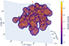 |
Fig. 1. Visual representation of our catalog of 100 voids in the local neighborhood within a distance of ≈200h−1 Mpc. The color scale represents the Voronoi overlap rate, i.e., how often a point is contained in a void in different realizations. This quantity is loosely related to the density profile of voids, with high values representing the innermost underdense regions, while lower values are at the edges. The clouds are truncated at the value of 0.37 in order to preserve the statistical volume of all voids. Finally, the wire-frame spheres mark the effective volume of each void. The Cartesian axes are centered on the observer, the xy plane corresponds to the equatorial plane, and the |

In Section 2 we present the constrained simulations we used as posterior samples of the Local Universe and the algorithm we used to extract voids from them. In Section 3 we describe the statistical method for detecting and characterizing high-significance voids, and in Section 4, we discuss the quality of the catalog we produced. In Section 5 we compare our results with known voids in the literature, and in Section 6, we discuss the whole work and present our conclusions.
2. Data products
To characterize the voids in our local neighborhood within z < 0.1, we used the Manticore Local posterior realizations of the Universe (McAlpine et al. 2025), a set of constrained N-body simulations of the large-scale structure, initialized to be consistent with the galaxy positions identified in the 2M++ data compilation (Lavaux & Hudson 2011). Produced in the Bayesian framework of the BORG algorithm, they represent 50 independent samples of the posterior distribution of the large-scale structure and allow us to carry out a complete statistical analysis of the voids. These constrained simulations will be made publicly available3.
2.1. The 2M++ galaxy compilation
The 2M++ compilation consists of ∼69 000 galaxies in our neighborhood, ranging up to redshift z < 0.1. It combines the galaxies from the photometric sample of the 2-Micron All-Sky Survey Extended Source (2MASS-XSC; Huchra et al. 2012), the spectroscopic redshifts of the 2MASS Redshift Survey (Huchra et al. 2012), the 6-Degree Field Galaxy Redshift Survey (Jones et al. 2006), and the Sloan Digital Sky Survey Data Release 7 (SDSS; Abazajian et al. 2009). The compilation is subdivided into eight bins of absolute magnitude in the K-band, with −25 ≤ MK < −21, while the angular completeness is characterized by a high-resolution, two-dimensional mask, which encodes the ratio of spectroscopic redshifts to photometric targets across the sky. This mask accounts for survey incompleteness due to bright sources on the foreground and the Galactic plane, as well as redshift completeness. These features are incorporated in the initial condition reconstruction of McAlpine et al. (2025): in order to account for the different completeness of the flux, the authors further sorted the galaxies into two apparent magnitude intervals, with 8 ≤ mK < 11.5 and 11.5 ≤ mK < 12.5. We refer to Lavaux & Hudson (2011) for further details on the data, and to McAlpine et al. (2025) for its use in BORG for the inference of the initial conditions.
2.2. Posterior realizations of the large-scale structure
The Manticore Local posterior simulations (McAlpine et al. 2025) are a set of posterior realizations of the large-scale structure describing the Local Universe in a Bayesian framework. They are produced following two separate procedures.
The first step consists of a Bayesian inference within the BORG algorithm. This probabilistic engine samples initial conditions of the Universe, evolves them to the present day distribution and constrains the realizations that are consistent with observed galaxy counts and positions. The initial power spectrum is computed with CLASS (Lesgourgues 2011), with the cosmological parameters inferred from the Dark Energy Survey year three (Abbott et al. 2022) ‘3x2pt + All Ext’. ΛCDM cosmology: h = 0.681, Ωm = 0.306, ΩΛ = 0.694, Ωb = 0.0486, As = 2.099 × 10⁻⁹, ns = 0.967, σ8 = 0.807.
We used a set of 50 independent posterior samples of the initial conditions (IC) that might have seeded the galaxy distribution in our local neighborhood at present day. They are represented on a box with side L = 1 Gpc = 681 h−1 Mpc, on a grid of N = 2563 voxels. The grid is then augmented to N = 10243 particles with mass resolution of 3.7 × 10¹⁰ M⊙. The IC are generated with second order Lagrangian Perturbation Theory (2LPT), and their evolution to z = 0 is computed with the SWIFT N-body solver (Schaller et al. 2024). Finally, structures are extracted from the present-day dark matter distribution using the HBT+ (Hierarchical Bound Tracing) subhalo finder (Han et al. 2012, 2018). The mass of the halos is defined as M200, crit, that is, the mass enclosed within r200, crit, the radius within which the mean enclosed density is 200 times the critical density of the Universe (200 × ρcrit). The result is 50 independent distributions, consisting of ∼1.3 × 10⁶ halos with resolution Mmin = 1012 M⊙, that can be then used as tracers to identify voids. We refer to the full Manticore paper (McAlpine et al. 2025) for further details regarding the construction of the constrained halo catalogs.
2.3. Independent void catalogs
We identified voids in the 50 samples using VIDE4 (Sutter et al. 2015), a void-finder that implements an enhanced version of ZOBOV (Neyrinck 2008) to construct voids with a watershed algorithm. VIDE computes a Voronoi tesselation of the tracers of the density field (in our case, halos) and merges the cells into zones and voids using the watershed transform (Platen et al. 2007). The resulting voids consist of the union of multiple cells, and they accordingly have complicated shapes, but can be summarized with their centers and effective radii. The center of a void is computed as the center of its cells, weighted by their volumes,
where xi and Vi are the position and volume of each Voronoi cell. The effective radius is
where V is the sum of the volume of all the Voronoi cells. These two properties are automatically computed by VIDE and printed in the final catalogs. Moreover, the code saves the volume of the Voronoi cells corresponding to each tracer, which can then be used to reconstruct the actual shape of each void.
We note that there is no unique definition of voids. As a consequence, the properties of these structures inevitably depend on the algorithm chosen to identify them. VIDE is one of the most established void finders in the literature, its features have been carefully tested (e.g., Sutter et al. 2014d,b), and it has been successfully employed in numerous independent works. It belongs to the family of watershed-based void finders, as described, for instance, by Platen et al. (2007), Neyrinck (2008). These kinds of void finders have characteristics that are best suited for our needs, as opposed to other void finders based on the union of spherical underdensities (Hoyle & Vogeley 2004; Padilla et al. 2005), or on the dynamics of the tracers of the density fields (Lavaux & Wandelt 2010; Cautun et al. 2013). The former category assumes that voids are unions of spheres, which facilitates their identification, at the cost of approximating their morphology; the latter reconstructs voids as sources of the velocity field, and it therefore contains information on the dynamics. It is challenging to obtain reliable velocity estimates from observation, however, and reconstructing them from simulations is computationally expensive. Additionally, these void finders miss the so-called voids-in-clouds (Sheth & van de Weygaert 2004), that is, underdense bubbles that are evolving into clustered structure, like walls, filaments or halos, where the velocities point inward to the center of the void, and they therefore appear to be overdense in the divergence field. VIDE provides a good trade-off between complexity in void morphology and computational performance. Catalogs of the 50 simulations boxes of Manticore-Local with periodic boundary conditions with ∼1.3 million halos each can be extracted in about a few hours.
Summary of the void properties for a few example voids.
3. Statistical void detection
We compared the 50 independent catalogs obtained from different realizations of the large-scale structure in order to identify the voids that occur multiple times in the same place. This is equivalent to detecting high-significance voids, which we will also dub as “true” voids for simplicity of presentation. A rigorous characterization of statistical significance is then described in Section 3.2.
Two voids belonging to the same cosmic web realization cannot overlap spatially due to the watershed void definition. A true void in the Universe is identified as an underdensity in multiple Markov chain Monte Carlo (MCMC) samples, however. Thus, placing all void centers from independent catalogs on the same shared three-dimensional space will produce clusters of points centered on real voids in the Universe. This signal can be noisy due to local minima of the density field being identified as voids by VIDE due to the scatter of tracers. For this reason, we only used the default catalog of VIDE, which excludes shallower voids with higher central density. This choice effectively reduced the risk of counting spurious ones, which are not well understood (Neyrinck 2008; Cousinou et al. 2019). We also chose to compare only similarly sized voids, which are more likely to be candidates for the same true void in the Universe.
The left panel of Fig. 2 shows the positions of the centers of voids with radius 30 < r < 50 h−1 Mpc on a slice of the 3D space, with thickness 60 h−1 Mpc. The blue circle represents the volume occupied by observed galaxies, up to a distance of ≈250 Mpc ≈ 170 h−1 Mpc, with the observer positioned in the center. For features in the matter distribution that are strongly supported by the data, independent posterior realizations of the large-scale structure show similarities, with voids of comparable sizes occupying the same regions of space. This is also evident when observing the average density of all realizations, as shown on the right panel of Fig. 2. The detection of stable voids between samples of the posterior reduces to a clustering problem.
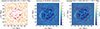 |
Fig. 2. Left panel: Centers of voids with radius 30 < r < 50 h−1 Mpc from all realizations, overlapped on a slice of the 3D space with thickness 60 h−1 Mpc. The dashed blue circle is centered on the observer, and it corresponds to a radius of ≈250 Mpc ≈ 170 h−1 Mpc, encompassing the volume with observed galaxies in 2M++ (where the constraints are more reliable) with interior points marked in red, and the other points plotted in orange. The unconstrained region outside the dashed black square presents a random distribution and can be used to assess the probability of having a cluster of n points by random chance. Central panel: Halo field averaged over all the MCMC realizations. The z thickness is 60 h−1 Mpc and matches the slice in the left panel. Right panel: Visual superposition of the two previous panels. |
3.1. Void-clustering algorithm
As mentioned in the beginning of Section 3, small and large voids detected from independent halo fields might happen to co-occur nearby in space, even without being different realizations of the same true void. A straightforward solution to prevent this problem is to sort voids into bins based on their radii, effectively only grouping together comparable ones.
In order to detect clusters among these similarly sized voids, we adopted the AgglomerativeClustering algorithm from the scikit-learn package5. This method belongs to the family of hierarchical clustering algorithms, and employs a bottom-up approach. In the first iteration, all points are clusters of a single member, and only those separated by the shortest distance start being merged. We chose to use the Ward distance, which minimizes the variance of the points that form a cluster. The linkage length is then gradually increased, either until all points are considered as part of the same cluster, or a stopping criterion is defined. This could be a fixed number of clusters or a maximum threshold distance. We enforced that the centers of voids should not be farther away from each other than their average radius. This guarantees that voids in a cluster overlap spatially. We chose the center of the radius bin as the threshold length.
3.2. Spurious void clusters and acceptance threshold
The clustering algorithm described so far accepts clusters on the basis of their scatter relative to their average size, yet it does not set any constraint on the number of members. Void centers that cannot be merged with many neighbors will make up clusters of just a few members. If not filtered out, they would be accepted as voids, despite carrying little to no statistical significance. An acceptance threshold is needed to discard these spurious clusters.
As shown in the left panel of Fig. 2, the outer part of the simulations is not constrained by data. The void centers in this region therefore varied freely between different realizations. As a result, the union of points from all realizations is spatially uncorrelated in the outer, unconstrained region. We counted the number of excess points that appeared in the neighborhood of each individual void center by pure chance, assuming a Poisson process to evaluate the associated probability. The circle represented in Figure 2 marks a radius of 250 Mpc ≈ 170 h−1 Mpc, roughly corresponding to the farthest galaxy observed in the 2M++ compilation. We observe some correlated structure even outside the edge of this boundary, however. In order to add some buffer, we considered a cube with side 600 Mpc = 408.6 h−1 Mpc centered on the observer. We used this volume as the interior of the simulation box, and all the voids outside of this region were used to estimate the occurrence of spurious clusters. While the constrained structure partially extends to the outer region of this buffer in the right panel of Fig. 2, this is only true for the thin slab we are plotting, and the concerned volume is negligible.
Given a particular radius bin, we selected the outer voids falling in this range and performed the clustering analysis described in Section 3.1. We could then count the occurrence of clusters of n ≥ 1 points to estimate the P(n − 1) Poisson distribution, and compute the value of nth corresponding to P(nth − 1) < pth, with pth an arbitrary threshold. In order to enforce very high statistical significance, we chose a threshold of pth = 6 × 10⁻⁷, that is, the conventional value of 5σ used in particle physics to claim a detection. We computed this threshold for different radius bins and rejected all the clusters that did not pass this acceptance criterion. This is a conservative choice that certainly excluded reasonably good candidate voids. The goal of this work is to describe real structures of the Universe, however, to produce a catalog of high-significance voids, albeit not exhaustive.
3.3. Continuous binning strategy
In addition to the detection of regions in our Local Universe that represent true voids, we are interested in probing the underlying probability distribution of their properties. Unfortunately, the width of the bins used in the clustering algorithm is an arbitrary choice that affects the voids we actually compare, impacting the estimated variance of the radius probability distribution we would infer from them. Moreover, for a given choice of bin width, the position of the edges may split a significant cluster, where members of the same true void get grouped into two different clusters that do not pass the significance test individually.
In order to overcome this problem, we fixed the width of our radius bins to a value ΔR, producing a window that we shifted continuously through the range of radii in our voids sample. In such a way, there is always a bin choice that prevents the splitting of significant clusters. With this strategy, voids with radii falling into the high density region of the underlying probability distribution belong to clusters that pass the acceptance criterion more often than others. Conversely, voids sampled from the tails of the distribution are grouped into smaller clusters that will be labeled as spurious ones. Counting how often each point is accepted assesses the importance of a single realization void in the evaluation of the statistical properties of the “true” void. This procedure produced a list of independent voids from different halo field realizations, with their respective weights. We inferred the underlying probability distribution with a weighted kernel density estimation (KDE). We used the gaussian_kde module from the scipy library6. A toy example of this procedure can be found in Appendix A and Figure A.1.
Unfortunately, this procedure is still sensitive to the choice of ΔR. Too small of a value prevents us from probing the full width of the radius distribution of larger voids, while choosing a too large value might mix together distinct voids that sit nearby, as in the common configuration of smaller satellite voids surrounding a large one. As a lower bound, we identified the size of the smallest void in the individual catalogs, Rmin ∼ 5 h−1 Mpc. Conversely, ΔR needs to be large enough to probe the width of the underlying distribution of the largest voids. Using the maximum value of the catalog as reference (Rmax ∼ 50 h−1 Mpc), we reasonably do not expect the standard deviation to reach half this value. We chose 25 h−1 Mpc as an upper bound for ΔR, and sampled in the middle of the range of [5, 25] h−1 Mpc, repeating the analysis with ΔR = 10, 12.5, 15, 17.5, 20 h−1 Mpc.
We considered the center value of ΔR = 15 h−1 Mpc as reference, and compared the catalog with the ones obtained with the perturbed choices of ΔR−− = 10 h−1 Mpc, ΔR− = 12.5 h−1 Mpc, ΔR+ = 17.5 h−1 Mpc and ΔR++ = 20 h−1 Mpc. As expected, the correspondence is not perfect, with voids disappearing when moving away from the reference catalog obtained with ΔR = 15 h−1 Mpc. We then selected the intersection of the five catalogs, consisting only of voids that are stable with respect to the choice of ΔR. This resulted in a final catalog of N = 100 high-significance voids.
4. Catalog analysis
We produced a catalog of 100 high-significance voids within a distance of ≈200 h−1 Mpc. The radius distribution is shown in Figure 3, where it is compared to the void population in the simulations. As a result of the weighting and KDE strategy detailed in Section 3.3, our catalog includes the probability distributions of position and radii. We can summarize their properties by computing the mean and standard deviation of these quantities. The complete results are presented in Appendix C, while some example voids are shown in Table 1. In our cartesian system the xy plane corresponds to the equatorial plane, while the  axis point to the equatorial north pole. The observer is located at [340.5, 340.5, 340.5]h−1 Mpc. We present the void centers in terms of equatorial sky coordinates (α, δ) and distance from us dc. The mean size
  of the void and its error is presented in column 6. We use this information to compute the redshift of the closest and farthest edges along the line of sight. In this section we proceed to analyze the quality of this catalog.
 |
Fig. 3. Histogram of the distribution of the void radii for the catalog of high-significance voids (blue) and for the average distribution of individual simulations (orange). The y-axis shows the actual number in each radius bin for the high-significance voids. The orange curve is arbitrarily rescaled to make it comparable. The two histograms illustrate how smaller voids in a single realization of the large-scale structure are more likely to be spurious or less significant, with only a fraction of them contributing to the final catalog. |
4.1. Shape characterization
In the discussion presented in Section 3, we simplified the shape of voids by treating them as spheres. VIDE is a watershed-based void finder that performs a Voronoi tessellation on the tracers of the density field and merges them though a watershed transform, however. As a result, the output voids are very irregularly shaped. We can use this information to retrieve the actual shape of the statistical voids.
In order to study the morphology of each individual void, we selected a box anchored in its center, with side equal to 4Rvoid, and grid it with resolution N = 323. By definition, every point in space is contained in the Voronoi cell corresponding to its closest tracer. Hence, we flagged as one every voxel whose closest tracer is part of a void, repeating the procedure for all the realizations that contribute to that specific void. We then averaged them using the appropriate weights introduced in Section 3.3. The result is a value between 0 and 1, that we define as the “Voronoi overlap rate” rVoro, describing how often a point belongs to the Voronoi cells of a realization of a void. The function defined on the whole space is closely related to the probability that the space around xc is part of the void, and hereafter we will refer to it as a Voronoi cloud.
An example void is presented in Fig. 4. The outskirts of its Voronoi cloud are unlikely to truly belong to the void, as they were identified as part of a void only in fewer halo field realizations. For all voids, we reduced the size of the clouds by truncating the points of the grid with Voronoi overlap rate of rVoro > rmin, testing different thresholds rmin. We evaluated the volumes of these subclouds, we converted them into the corresponding radii, and we compared them to the mean posterior of the radii distributions obtained from the KDEs. We observed that the dependence between the two quantities is linear, as detailed in Appendix B and shown in Fig. B.1. In particular, choosing rmin = 0.37 we found that the ratio of the two definitions of void radius equals 1.0004 ∼ 1 within subpercent accuracy. We adopted this threshold in order to determine whether a point belongs to a void, effectively characterizing the actual shape of the void, without overestimating its volume. Additionally, this method can be used to probe the deeper interior of voids by applying a further truncation with rmin > 0.37, as shown in Fig. B.2 of Appendix B.
 |
Fig. 4. Left panel: Full Voronoi cloud of an example void around its center. The color scale represents the Voronoi overlap rate, ranging from 0 to 1, i.e., how likely a point is to belong to the void throughout different realizations. This value is loosely related to the actual underlying probability distribution, with the yellow regions corresponding to the innermost underdense environment. The wire-frame sphere in the middle represents the effective volume of the void, and the Voronoi cloud extends significantly beyond this region. Right panel: Voronoi cloud truncated to make values of Voronoi overlap rate greater than 0.37, as interpolated from the linear fit of Figure B.1 in Appendix B. The outskirts are removed, and the remaining cloud conserves the mean volume inferred from the Bayesian analysis, while still retaining information on the shape of the void. |
In order to visualize the spatial interplay and connections between these individual voids, we can paint their Voronoi clouds onto the whole volume. We defined a grid of 643 voxels, with coarser resolution of ∼7.4 h−1 Mpc. We then assigned each point of the single Voronoi clouds to the closest voxel, averaging the multiple contributions in the cases where multiple voxels of an individual void cloud fall into a single voxel of the global grid. We then chose rVoro = 0.37 as the threshold that conserves the mean volume of all voids within subpercent error, yielding a ratio of 0.995. The global Voronoi cloud for all voids is shown in Fig. 1.
4.2. Average properties
In order to develop the optimal void clustering strategy for our problem, we carried out a blind analysis without adjusting our choices to the underlying halo fields. We now compare the statistical voids of our catalog to the mean halo distribution to check their consistency. We assess the quality of our detection through visual inspection. For each void, we selected the truncated Voronoi cloud with rVoro > 0.37, we summed the overlap rate on the z direction, and we normalized the result to have a value between 0 and 1. This is qualitatively equivalent to marginalizing the probability distribution over the z direction. We plot a slice of the halo field averaged over all realizations, with thickness equal to Rvoid, and we overlap the contours corresponding to 0 and 0.5 marginal Voronoi overlap rate. In Fig. 5 we show an example void. We find a good qualitative match between the void profile and its density environment, as the void is not only centered in an under-dense region, but the contours follow the shape of the underlying structures.
 |
Fig. 5. Representation of void 10, our best candidate to be the well-known Local Void, on a slice of the average halo field with thickness equal to the effective radius Rvoid. The yellow star represents the mean posterior of the center, while the circle is as large as the mean effective volume. The black contours represent the truncated Voronoi cloud, i.e., all the points with rVoro > 0.37, marginalized over the line of sight, obtained by summing the values over the z direction. We normalized this probability distribution to a range between 0 and 1, the contour lines are the 0 and 0.5 levels. The profiles follow perfectly the structure of the underlying field, confirming the quality of the reconstruction. However, the projection does not fully capture the three dimensional information, and heavily depends on the thickness of the density field slab. A representation of different slices on the z-axis can be found at this link: https://voids.cosmictwin.org |
Finally, we can visualize the full catalog using the spherical approximation. In Fig. 6 we represent the sky at redshift 0.03 < z < 0.035 and 0.035 < z < 0.04, representing the galaxies of the 2M++ compilation and the void centers on top of it. The solid circles represent the angular size of the effective radius projected on the sky at the center’s redshift; the semitransparent circles represent the intersection with voids centered in adjacent redshift bins. The remaining redshift bins are shown in Figure C.1 in Appendix C.
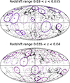 |
Fig. 6. Sky representation in Galactic coordinates, with the zero longitude point in the center, in two adjacent redshift slices with 0.03 < z < 0.035 and 0.035 < z < 0.04. The black dots represent the 2M++ galaxies used to infer the posterior realizations of the Local Universe. The crosses represent the void centers within the redshift bin, while the solid circles are the apparent size of their effective radii. The semitransparent circles represent the intersection with voids centered in adjacent redshift bins. We show the neighboring voids only when they intersect the redshift bin entirely, to minimize the visual contamination from galaxies outside of the void. Additionally, the spherical approximation becomes less accurate the farther away from the void center. As a visual confirmation, voids actually occupy the regions with little to no galaxies. The predictive power of the Manticore-Local suite combined with our void finding procedure is shown by the fact that we are able to infer voids behind the Galactic plane, in regions where we do not have direct observations of galaxies. The remaining redshift slices are shown in Figure C.1 in Appendix C. A movie is available online [VoidsGalacticCoord.gif]. |
5. Comparison with voids in the literature
In this section, we compare our catalog to the known voids that were previoulsy identified by astronomers with observational methods. This task is nontrivial, as voids not only subtend great angles in the sky, but they are also interconnected. This prevents a clear definition of their centers and boundaries. They are often named after the constellation that lies in front of them for practical purposes, but there is no indisputable catalog of voids the community agrees upon. We proceed in a qualitative comparison with previous works in the tradition of astronomers analyzing sky maps and producing catalogs of named objects; for this reason, we do not consider statistical void catalogs extracted running a void finder on a particular galaxy sample. The voids from our catalog mentioned in the following sections are all summarized in Table 1.
5.1. Dynamical void detection
Tully et al. (2019) characterized the shape and interplay of voids, by analyzing the velocities of the surrounding galaxies to reconstruct the underlying density field, using the Cosmicflows-3 dataset (Tully et al. 2016). We compare with the 25 local minima they identified, classified as part of the Local Void, the Hercules void, the Sculptor void, and the Eridanus void. We first converted their coordinates into our simulation volume, and evaluated the Voronoi cloud in these points. We considered the Voronoi overlap rate of the eight closest voxels of the grid representation, and averaged them using the inverse of the distance as weights. If the estimated value was higher than the acceptance threshold of 0.37, we flagged the candidate point as part of a void. We find that 17 out of 25 pass the acceptance threshold, corresponding to a 68% confirmation rate.
As a first cross-check, we compare the remaining eight points to the mean halo field, and we do not find significant overdensities overlapping to those regions. Out of the rejected points, seven present a low value of the Voronoi overlap rate (≲ 0.2), and are located at a significant distance from our global Voronoi cloud. These points are still likely to be their own independent underdensities, but their significance is lower than our designated 5σ threshold. The remaining point (named “Lacerta-2.4” in the reference paper) sits close to the boundaries of the global Voronoi cloud, at a distance of a few h−1 Mpc, despite not strictly belonging to any void of our catalog. These differences can be due to the −∇⋅v estimation of the density, as the two fields de-correlate below the ∼50% level at scales smaller than ∼10 − 15 h−1 Mpc (Hahn et al. 2015). Accounting for these sources of discrepancy, our overall agreement to dynamic voids is good.
As far as it concerns the Local Void, we find good agreement for the point marked as “Aquila-0.8” point, which is part of void 10 of our catalog. The “Andromeda-2.3” point is fully inside void 75 of our catalog, while the aforementioned “Lacerta-2.4” is located close to its edge. This spatial distribution matches the full visualization of the void in Tully et al. (2019). This comparison highlights how what is commonly referred to as the Local Void is the connection of separate voids.
5.2. The Local Void
The Local Void is hard to characterize because it lies partially behind the Galactic plane and subtends a large portion of the sky due to its vicinity. First discovered by Tully & Fisher (1987), different works have defined different positions for its center.
Karachentseva et al. (1999, 2002) locate its center at α = 18h38m, δ = 18°, and redshift range < 1500 kms−1; while Nakanishi et al. (1997) estimate the center of the Local Void at l ∼ 60°, b ∼ −15° (i.e., α ∼ 20h40m, δ ∼ 16°), its distance at cz ∼ 2500 kms−1, and the size of the void along the line of sight as cz ∼ 2500 kms−1. As the boundaries of the Local Void are not unequivocally defined, different authors happen to use the same name to refer to different regions. Karachentseva et al. (1999) point out the vicinity of these two separate voids, that can thus be confused as the same Local Void, and distinguish them by calling them, respectively, the “Hercules-Aquila Void” and the “Pegasus-Delphinus Void”. We do not find this separation in our catalog, however, because they overlap with void 10, whose center is located at α ∼ 18h05m, δ ∼ −16°, and redshift 3900kms−1, as shown in Table 1. With its center at a distance of ∼39 h−1 Mpc and radius of ∼34 h−1 Mpc, this void is confirmed to be our best candidate of the Local Void.
Additionally, Einasto et al. (1994) defined the northern Local Void (NLV) as centered in α = 256.1°, δ = −4.8°, at a distance of 61 h−1 Mpc away from us, and with a radius of 52 h−1 Mpc. Void 10 of our catalog overlaps perfectly within its range, but it only extends to a distance of ∼73 h−1 Mpc. Towards the farthest edge of this region, we find void 83, with a smaller radius of ∼14 h−1 Mpc and connected to void 10 through a bridge. The volume claimed by the authors is much larger than other accounts of the Local Void, and it extends farther away from us. However they looked for empty regions in the distribution of clusters of galaxies, which are a much sparser tracer of the desnity field than the galaxies themselves: as finer structures like filaments are not resolved, smaller adjacent voids appear to be a larger one. As opposed to the northern Local Void, Einasto et al. (1994) also mention a southern Local Void (SLV), centered in α = 121.7°, δ = −1.5°, at a distance of 96 h−1 Mpc away from us, and with a radius of 56 h−1 Mpc. We found no significant underdensities in this direction, however.
5.3. Other voids
Historically, the first void detection is attributed to Gregory & Thompson (1978), who noticed a region devoided of galaxies behind the Coma/A1367 supercluster. Void 45 in our catalog matches the sky coordinates, and the redshift range of 5000 − 6200 km s−1, as shown in Table 1. Early records of voids in the Local Universe can be found in Kirshner et al. (1981). Void 88 of our catalog is centered in the Boötes constellation7 and extends on a redshift range of 10 000 − 18 100 km s−1, overlapping with the void claimed by the authors. Similarly, the Pisces void marginally matches void 15, while void 75 extends in the Perseus/Pisces region defined in the reference. It is worth noting that the latter is very nearby, at a distance of ∼33 h−1 Mpc, and in fact it can be considered part of the Local Void of Tully et al. (2019), as described in Section 5.1.
The work by Kirshner et al. (1981) also mentions a void in the Hercules constellation, in the redshift range of 5500 − 8500 km s−1, while Freudling et al. (1991) studied a very nearby region, with ranges 14h < α < 17h, 10° < δ < 60° and redshift 4900 − 8900 km s−1; conversely, Krumm & Brosch (1984) define a very narrow Hercules region (15h45m < α < 16h15m, 14° < δ < 22°) at approximately the same redshift range, as well as claiming a Perseus void at 0h < α < 2h, 0° < δ < 20° and redshift 6500 − 9500 km s−1. We do not find high-significance voids in any of those regions.
Other named voids can be found in Willmer et al. (1995), who report the Hydra void in the region centered in α = 11h, δ = −30°, and redshift range 4500 − 6000 km s−1. This volume corresponds to our void 57, which however extends up to redshift ∼9400 kms−1. The same authors mention the Leo void at α = 11h30m and redshift 4000 kms−1 in the declination range of −10° < δ < 10°, which overlaps perfectly with void 28 of our catalog. Finally, Pustilnik et al. (2006) studied the Pegasus void as defined by Fairall (1998), with coordinates of the center in α = 22h, δ = 15°, and cz = 5500 kms−1. We found no match with any of our voids in the range of cz = 3000 kms−1 that was mentioned by the authors, however.
5.4. Final remarks on the comparison
In conclusion, the centers and boundaries of voids in surveys are not always precisely defined, hence our comparison is mostly qualitative. In the literature voids are often identified as regions with little to no galaxies, which tend to be smaller in size compared to voids in halos or dark matter, as the latter still contain some galaxies. Overall, we find a good match with the known voids discovered observationally by astronomers. Our catalog is not exhaustive, however, because our acceptance threshold is very high due to the 5σ criterion: observed voids that do not match our work are not disproved, as they are likely to be real but slightly less significant. Conversely, the strictness of our criterion makes us confident that the voids we claim are real, and can be used for any applications that needs a characterization of the density environment of astronomical objects. Finally, for practical reasons our comparison is with respect to a limited selection of works on observational voids, as we chose to restrict ourselves to those that are regularly referred to with a proper name in the literature. We are therefore aware of potentially missing relevant sources, including all the common catalogs extracted by running a void finder on a galaxy sample: this type of catalog holds higher statistical power in aggregate, but individual voids are more subject to statistical and systematic uncertainty.
6. Discussion and conclusions
We presented a catalog of high-significance cosmic voids extracted from constrained simulations of the Local Universe. For our analysis, we used the Manitcore-Local suite from McAlpine et al. (2025), which is a set of 50 N-body simulations initialized with the primordial density field inferred with the BORG algorithm (Jasche & Wandelt 2013; Jasche & Lavaux 2019). Produced in a Bayesian framework, they represent independent statistical realizations of the posterior distribution of the cosmic web. To characterize the predicted structures, we ran the VIDE void finder (Sutter et al. 2015) on the halos from each individual realization and obtained a set of 50 independent void catalogs. We overlapped the centers of these voids in the three-dimensional space and found notable clusters of points in particular locations, as shown in Figure 2. These clusters correspond to the regions that are most likely to be real voids in the dark matter distribution.
We developed the optimal clustering strategy to identify the void clusters in an unbiased way, avoiding arbitrary choices of free parameters. We evaluated the statistical significance of each detection by modeling the probability of void clusters that emerge in the union of uncorrelated realizations of the large-scale structure through a Poisson process. We rejected spurious void clusters by imposing a 5σ detection threshold, that is, we only accepted clusters that could have occurred by random chance with a probability of ∼6 × 10⁻⁷. The result of this work is a catalog of 100 voids that consist of posterior distributions of their center positions and radii. Their main properties can be found in Appendix C for the complete catalog, and some notable voids are summarized in Table 1. This statistical result only considered the effective volume of voids, which is equivalent to approximating them as spheres. The VIDE algorithm finds voids through a Voronoi tesselation of the tracers of the density field, however, and identifies cells to be merged into zones and voids using the watershed transform (Platen et al. 2007). This yields very complex morphologies. We used this information to reconstruct the full shape of voids, as presented in Figure 4 for an example void and in Figure 1 for the whole catalog. Further visualizations can be found on the dedicated website8, and the catalog is publicly available for download9.
To determine the quality of the voids in our catalog, we compared them directly to the mean posterior of the underlying halo field. The overall consistency between the profile of the voids and the density environment is good, as shown in Figure 5 for an example void. The reliability of the catalog therefore strongly depends on the quality of the Manticore-Local simulations and their posterior predictions. The reconstruction of the initial conditions of the Universe through BORG is now a well-established tool for field-level cosmology. Ever since its first publication by Jasche & Wandelt (2013), the algorithm has seen notable improvements, passed several consistency tests, and has undergone continuous refinements to remain state-of-the-art technology (we refer to Jasche et al. (2015), Lavaux & Jasche (2016), Jasche & Lavaux (2019), Lavaux et al. (2019) for further details). As a second check, the Manticore-Local simulations were carefully tested to be consistent with the cosmological model, to predict known galaxy clusters, and to reconstruct the velocity field could, as detailed in McAlpine et al. (2025).
Possible sources of bias in the procedure can occur when the chains are not fully converged and the samples are correlated. These issues would affect the outer regions of the box in particular, which are not constrained by data, where the Gaussian prior on the initial conditions is the predominant element of the inference. McAlpine et al. (2025) addressed this possibility by running five independent MCMC chains that passed the Gelman-Rubin convergence test. In addition, the 50 samples of the final Manticore-Local set were taken at a sufficient separation along the chains to be uncorrelated. As a further confirmation, the right panel of Figure 2 shows that the exterior of the box does not present significant structure, with a a density contrast close to zero. This visually illustrates that the MCMC chains converged. For our purposes, the samples can be safely treated as independent realizations of the posterior distribution of the large-scale structure.
One possible limitation of this work is the use of a single void-finding algorithm instead of verifying the consistency of the results with respect to different choices. As discussed in Section 2.3, however, VIDE is not only a well-established, carefully tested, and widely used tool in the void literature, but also presents desirable features, such as shape agnosticism and a high computational performance on simulations. Our void-clustering strategy only considered first-order properties of voids, that is, center positions and sizes. These are overall consistent among void finders, at least for the largest voids (Colberg et al. 2008). It is reasonable to expect comparable results for different void definitions. Possible outlier voids emerging due to the specific characteristics of a particular algorithm are expected to be rejected by the 5σ detection threshold. The probabilistic nature of the procedure might attenuate the difference between void finders, making the catalog robust to these variations. These claims need to be tested in future works.
Finally, we compared our catalogs with different reports of observational detections of voids in the literature. We considered underdensities inferred from velocity measurements by Tully et al. (2019), as well as voids identified as regions with only a few to no galaxies. Taking into account the intrinsic challenges of the comparison, that is, the fundamental differences of the procedures, and the not well-defined centers and boundaries, the overall agreement with the references we considered is good. Our catalog only contains voids with a very high statistical significance, and it is therefore not exhaustive. We are aware that we probably missed real voids due to the strictness of our selection, and we therefore do not disprove other accounts of known voids that do not appear in our catalog.
In conclusion, this work introduces a viable benchmark for identifying cosmic voids in the Local Universe and for assessing their statistical significance. We produced a catalog of voids that are real structures in the dark matter distribution and eliminated spurious voids that typically occur from a direct detection from galaxy surveys. Our method allowed us to infer the posterior distributions of void properties in a Bayesian framework, and we obtained an estimate of their statistical uncertainties. Additionally, our voids have well-defined centers, shapes, and boundaries, which make the catalog practical to use for all applications that need characterization of the density environment, including galaxy properties, their evolution, and galaxy biasing. As traditional watershed voids extend to the surrounding filaments and walls, the galaxies occupying these overdense regions might be misclassified as void galaxies and might contaminate the signal (Zaidouni et al. 2025). Although they originate from the same technique, our voids can be truncated to their deeper interior, as described in Section 4.1. This is a useful feature to prevent this systematic issue. Beyond galaxies, further environment-based applications include supernovae and their use for measurements of the Hubble constant, and high-energy astrophysics, such as black holes and AGNs in voids. We make the catalog publicly available10 and encourage researchers from different fields of astronomy to download it and use it for their work.
Ongoing efforts within the Aquila consortium will produce constrained simulations on larger volumes, called Manticore-Deep, to leverage the information from a larger galaxy survey such as the SDSS. We expect to extract a larger number of voids from these suites due to volume scaling, which will characterize the deeper Universe and increase the statistical power of this probe. This can be used for cosmology through cross correlations with the large-scale structure through the weak gravitational lensing of galaxies, or with the cosmic microwave background. Possible tests for this latter case include the late-time integrated Sachs-Wolfe (ISW) effect, the thermal and kinematic Sunyaev-Zel’dovich (SZ) effect, or a direct comparison with the density maps reconstructed from cosmic shear.
Movies
Movie 1 associated with Fig. 6 Access Supplementary Material
Movie 2 associated with Fig. A.1 Access Supplementary Material
Data availability
Movies associated to Figs. 6, A.1, and C.1 are available at https://www.aanda.org
The Manticore-Local constrained simulations will be publicly available11. We provide supplementary visualizations for this work on the public website12, while the derived void catalog can be downloaded13 and used by the1415 community.
Acknowledgments
We thank Paul Sutter, Alice Pisani, Florent Leclercq, Clotilde Laigle, R. Brent Tully, and Ali Rida Khalife for useful comments and discussions. This work has been done within the Aquila Consortium and the Simons Collaboration on “Learning the Universe”. This work has made use of the Infinity Cluster hosted by Institut d’Astrophysique de Paris; the authors acknowledge Stéphane Rouberol for his efficient management of this facility. This work benefitted from the HPC resources of TGCC (Trés Grand Centre de Calcul), Irene-Joliot-Curie supercomputer, under the allocations A0170415682 and SS010415380. JJ, GL, and SM acknowledge support from the Simons Foundation through the Simons Collaboration on “Learning the Universe”. This work was made possible by the research project grant “Understanding the Dynamic Universe”, funded by the Knut and Alice Wallenberg Foundation (Dnr KAW 2018.0067). Additionally, JJ acknowledges financial support from the Swedish Research Council (VR) through the project “Deciphering the Dynamics of Cosmic Structure” (2020-05143). BDW acknowledges support from the DIM ORIGINES 2023 “INFINITY NEXT” grant. The Flatiron Institute is a division of the Simons Foundation.
References
- Abazajian, K. N., Adelman-McCarthy, J. K., Agüeros, M. A., et al. 2009, ApJS, 182, 543 [Google Scholar]
- Abbott, T. M. C., Aguena, M., Alarcon, A., et al. 2022, Phys. Rev. D, 105, 023520 [CrossRef] [Google Scholar]
- Alcock, C., & Paczynski, B. 1979, Nature, 281, 358 [NASA ADS] [CrossRef] [Google Scholar]
- Aubert, M., Cousinou, M.-C., Escoffier, S., et al. 2022, MNRAS, 513, 186 [NASA ADS] [CrossRef] [Google Scholar]
- Aubert, M., Rosnet, P., Popovic, B., et al. 2025, A&A, 694, A7 [NASA ADS] [CrossRef] [EDP Sciences] [Google Scholar]
- Banerjee, R., & Jedamzik, K. 2004, Phys. Rev. D, 70, 123003 [NASA ADS] [CrossRef] [Google Scholar]
- Barreira, A., Cautun, M., Li, B., Baugh, C. M., & Pascoli, S. 2015, JCAP, 2015, 028 [Google Scholar]
- Bayer, A. E., Villaescusa-Navarro, F., Massara, E., et al. 2021, ApJ, 919, 24 [NASA ADS] [CrossRef] [Google Scholar]
- Beygu, B., Kreckel, K., van der Hulst, J. M., et al. 2016, MNRAS, 458, 394 [NASA ADS] [CrossRef] [Google Scholar]
- Biswas, R., Alizadeh, E., & Wandelt, B. D. 2010, Phys. Rev. D, 82, 023002 [NASA ADS] [CrossRef] [Google Scholar]
- Bos, E. G. P., van de Weygaert, R., Dolag, K., & Pettorino, V. 2012, MNRAS, 426, 440 [NASA ADS] [CrossRef] [Google Scholar]
- Cai, Y.-C., Neyrinck, M. C., Szapudi, I., Cole, S., & Frenk, C. S. 2014, ApJ, 786, 110 [NASA ADS] [CrossRef] [Google Scholar]
- Cai, Y.-C., Padilla, N., & Li, B. 2015, MNRAS, 451, 1036 [NASA ADS] [CrossRef] [Google Scholar]
- Cai, R.-G., Ding, J.-F., Guo, Z.-K., Wang, S.-J., & Yu, W.-W. 2021, Phys. Rev. D, 103, 123539 [NASA ADS] [CrossRef] [Google Scholar]
- Camarena, D., Marra, V., Sakr, Z., & Clarkson, C. 2022, Class. Quantum Gravity, 39, 184001 [Google Scholar]
- Castello, S., Högås, M., & Mörtsell, E. 2022, JCAP, 2022, 003 [CrossRef] [Google Scholar]
- Cautun, M., van de Weygaert, R., & Jones, B. J. T. 2013, MNRAS, 429, 1286 [NASA ADS] [CrossRef] [Google Scholar]
- Ceccarelli, L., Duplancic, F., & Garcia Lambas, D. 2022, MNRAS, 509, 1805 [Google Scholar]
- Chan, K. C., Hamaus, N., & Biagetti, M. 2019, Phys. Rev. D, 99, 121304 [CrossRef] [Google Scholar]
- Clampitt, J., Cai, Y.-C., & Li, B. 2013, MNRAS, 431, 749 [NASA ADS] [CrossRef] [Google Scholar]
- Colberg, J. M., Pearce, F., Foster, C., et al. 2008, MNRAS, 387, 933 [NASA ADS] [CrossRef] [Google Scholar]
- Contarini, S., Ronconi, T., Marulli, F., et al. 2019, MNRAS, 488, 3526 [NASA ADS] [CrossRef] [Google Scholar]
- Contarini, S., Marulli, F., Moscardini, L., et al. 2021, MNRAS, 504, 5021 [NASA ADS] [CrossRef] [Google Scholar]
- Contarini, S., Verza, G., Pisani, A., et al. 2022, A&A, 667, A162 [NASA ADS] [CrossRef] [EDP Sciences] [Google Scholar]
- Contarini, S., Pisani, A., Hamaus, N., et al. 2023, ApJ, 953, 46 [NASA ADS] [CrossRef] [Google Scholar]
- Cousinou, M. C., Pisani, A., Tilquin, A., et al. 2019, Astron. Comput., 27, 53 [NASA ADS] [CrossRef] [Google Scholar]
- D’Amico, G., Musso, M., Noreña, J., & Paranjape, A. 2011, Phys. Rev. D, 83, 023521 [Google Scholar]
- Davies, C. T., Cautun, M., Giblin, B., et al. 2021, MNRAS, 507, 2267 [NASA ADS] [Google Scholar]
- de Lapparent, V., Geller, M. J., & Huchra, J. P. 1986, ApJ, 302, L1 [Google Scholar]
- Dekel, A., & Silk, J. 1986, ApJ, 303, 39 [Google Scholar]
- Desmond, H., Hutt, M. L., Devriendt, J., & Slyz, A. 2022, MNRAS, 511, L45 [Google Scholar]
- Di Valentino, E., Mena, O., Pan, S., et al. 2021, CQG, 38, 153001 [NASA ADS] [CrossRef] [Google Scholar]
- Ding, Q., Nakama, T., & Wang, Y. 2020, Sci. China Phys. Mech. Astron., 63, 290403 [Google Scholar]
- Domínguez-Gómez, J., Pérez, I., Ruiz-Lara, T., et al. 2023, Nature, 619, 269 [CrossRef] [Google Scholar]
- Douglass, K. A., Veyrat, D., & BenZvi, S. 2023, ApJS, 265, 7 [NASA ADS] [CrossRef] [Google Scholar]
- Eder, J. A., Schombert, J. M., Dekel, A., & Oemler, A., Jr 1989, ApJ, 340, 29 [Google Scholar]
- Einasto, M., Einasto, J., Tago, E., Dalton, G. B., & Andernach, H. 1994, MNRAS, 269, 301 [Google Scholar]
- Fairall, A. P. 1998, Large-scale structures in the universe [Google Scholar]
- Falck, B., Koyama, K., Zhao, G.-B., & Cautun, M. 2018, MNRAS, 475, 3262 [NASA ADS] [CrossRef] [Google Scholar]
- Freudling, W., Martel, H., & Haynes, M. P. 1991, ApJ, 377, 349 [Google Scholar]
- García-Bellido, J., & Haugbølle, T. 2008, JCAP, 2008, 016 [CrossRef] [Google Scholar]
- Geller, M. J., & Huchra, J. P. 1989, Science, 246, 897 [NASA ADS] [CrossRef] [Google Scholar]
- Granett, B. R., Neyrinck, M. C., & Szapudi, I. 2008, ApJ, 683, L99 [NASA ADS] [CrossRef] [Google Scholar]
- Gregory, S. A., & Thompson, L. A. 1978, ApJ, 222, 784 [NASA ADS] [CrossRef] [Google Scholar]
- Habouzit, M., Pisani, A., Goulding, A., et al. 2020, MNRAS, 493, 899 [NASA ADS] [CrossRef] [Google Scholar]
- Hahn, O., Angulo, R. E., & Abel, T. 2015, MNRAS, 454, 3920 [Google Scholar]
- Hamaus, N., Sutter, P. M., & Wandelt, B. D. 2014a, Phys. Rev. Lett., 112, 251302 [NASA ADS] [CrossRef] [Google Scholar]
- Hamaus, N., Wandelt, B. D., Sutter, P. M., Lavaux, G., & Warren, M. S. 2014b, Phys. Rev. Lett., 112, 041304 [NASA ADS] [CrossRef] [Google Scholar]
- Hamaus, N., Sutter, P. M., Lavaux, G., & Wandelt, B. D. 2015, JCAP, 2015, 036 [Google Scholar]
- Hamaus, N., Pisani, A., Sutter, P. M., et al. 2016, Phys. Rev. Lett., 117, 091302 [NASA ADS] [CrossRef] [Google Scholar]
- Hamaus, N., Pisani, A., Choi, J.-A., et al. 2020, JCAP, 2020, 023 [Google Scholar]
- Hamaus, N., Aubert, M., Pisani, A., et al. 2022, A&A, 658, A20 [NASA ADS] [CrossRef] [EDP Sciences] [Google Scholar]
- Han, J., Jing, Y. P., Wang, H., & Wang, W. 2012, MNRAS, 427, 2437 [NASA ADS] [CrossRef] [Google Scholar]
- Han, J., Cole, S., Frenk, C. S., Benitez-Llambay, A., & Helly, J. 2018, MNRAS, 474, 604 [CrossRef] [Google Scholar]
- Haslbauer, M., Banik, I., & Kroupa, P. 2020, MNRAS, 499, 2845 [Google Scholar]
- Hoeft, M., Yepes, G., Gottlöber, S., & Springel, V. 2006, MNRAS, 371, 401 [NASA ADS] [CrossRef] [Google Scholar]
- Hoscheit, B. L., & Barger, A. J. 2018, ApJ, 854, 46 [NASA ADS] [CrossRef] [Google Scholar]
- Hosking, D. N., & Schekochihin, A. A. 2023, Nat. Commun., 14, 7523 [Google Scholar]
- Hoyle, F., & Vogeley, M. S. 2004, ApJ, 607, 751 [NASA ADS] [CrossRef] [Google Scholar]
- Hoyle, F., Rojas, R. R., Vogeley, M. S., & Brinkmann, J. 2005, ApJ, 620, 618 [NASA ADS] [CrossRef] [Google Scholar]
- Hoyle, F., Vogeley, M. S., & Pan, D. 2012, MNRAS, 426, 3041 [NASA ADS] [CrossRef] [Google Scholar]
- Huchra, J., Davis, M., Latham, D., & Tonry, J. 1983, ApJS, 52, 89 [NASA ADS] [CrossRef] [Google Scholar]
- Huchra, J. P., Macri, L. M., Masters, K. L., et al. 2012, ApJS, 199, 26 [Google Scholar]
- Hui, L., Nicolis, A., & Stubbs, C. W. 2009, Phys. Rev. D, 80, 104002 [NASA ADS] [CrossRef] [Google Scholar]
- Hutschenreuter, S., Dorn, S., Jasche, J., et al. 2018, CQG, 35, 154001 [Google Scholar]
- Ichiki, K., Yoo, C.-M., & Oguri, M. 2016, Phys. Rev. D, 93, 023529 [Google Scholar]
- Ilić, S., Langer, M., & Douspis, M. 2013, A&A, 556, A51 [NASA ADS] [CrossRef] [EDP Sciences] [Google Scholar]
- Inoue, K. T., & Silk, J. 2007, ApJ, 664, 650 [Google Scholar]
- Jasche, J., & Lavaux, G. 2019, A&A, 625, A64 [NASA ADS] [CrossRef] [EDP Sciences] [Google Scholar]
- Jasche, J., & Wandelt, B. D. 2013, MNRAS, 432, 894 [Google Scholar]
- Jasche, J., Leclercq, F., & Wandelt, B. D. 2015, JCAP, 2015, 036 [Google Scholar]
- Jõeveer, M., Einasto, J., & Tago, E. 1978, MNRAS, 185, 357 [Google Scholar]
- Jones, D. H., Peterson, B. A., Colless, M., & Saunders, W. 2006, MNRAS, 369, 25 [Google Scholar]
- Kamionkowski, M., Verde, L., & Jimenez, R. 2009, JCAP, 2009, 010 [Google Scholar]
- Karachentsev, I. D., Sharina, M. E., Makarov, D. I., et al. 2002, A&A, 389, 812 [NASA ADS] [CrossRef] [EDP Sciences] [Google Scholar]
- Karachentseva, V. E., Karachentsev, I. D., & Richter, G. M. 1999, A&AS, 135, 221 [NASA ADS] [CrossRef] [EDP Sciences] [Google Scholar]
- Kenworthy, W. D., Scolnic, D., & Riess, A. 2019, ApJ, 875, 145 [NASA ADS] [CrossRef] [Google Scholar]
- Kirshner, R. P., Oemler, A., Jr, Schechter, P. L., & Shectman, S. A. 1981, ApJ, 248, L57 [NASA ADS] [CrossRef] [Google Scholar]
- Korochkin, A., Neronov, A., Lavaux, G., Ramsøy, M., & Semikoz, D. 2022, J. Exp. Theor. Phys., 134, 498 [NASA ADS] [CrossRef] [Google Scholar]
- Kovács, A., Sánchez, C., García-Bellido, J., et al. 2019, MNRAS, 484, 5267 [CrossRef] [Google Scholar]
- Kraljic, K., Arnouts, S., Pichon, C., et al. 2018, MNRAS, 474, 547 [Google Scholar]
- Krause, E., Chang, T.-C., Doré, O., & Umetsu, K. 2013, ApJ, 762, L20 [NASA ADS] [CrossRef] [Google Scholar]
- Kreckel, K., Platen, E., Aragón-Calvo, M. A., et al. 2011, AJ, 141, 4 [NASA ADS] [CrossRef] [Google Scholar]
- Kreisch, C. D., Pisani, A., Carbone, C., et al. 2019, MNRAS, 488, 4413 [NASA ADS] [CrossRef] [Google Scholar]
- Kreisch, C. D., Pisani, A., Villaescusa-Navarro, F., et al. 2022, ApJ, 935, 100 [NASA ADS] [CrossRef] [Google Scholar]
- Krumm, N., & Brosch, N. 1984, AJ, 89, 1461 [Google Scholar]
- Lam, T. Y., Sheth, R. K., & Desjacques, V. 2009, MNRAS, 399, 1482 [Google Scholar]
- Lavaux, G., & Hudson, M. J. 2011, MNRAS, 416, 2840 [Google Scholar]
- Lavaux, G., & Jasche, J. 2016, MNRAS, 455, 3169 [Google Scholar]
- Lavaux, G., & Wandelt, B. D. 2010, MNRAS, 403, 1392 [NASA ADS] [CrossRef] [Google Scholar]
- Lavaux, G., & Wandelt, B. D. 2012, ApJ, 754, 109 [NASA ADS] [CrossRef] [Google Scholar]
- Lavaux, G., Jasche, J., & Leclercq, F. 2019, ArXiv e-prints [arXiv:1909.06396] [Google Scholar]
- Lazar, I., Kaviraj, S., Martin, G., et al. 2023, MNRAS, 520, 2109 [NASA ADS] [CrossRef] [Google Scholar]
- Leclercq, F., Jasche, J., Sutter, P. M., Hamaus, N., & Wandelt, B. 2015, JCAP, 2015, 047 [Google Scholar]
- Lee, J., & Park, D. 2009, ApJ, 696, L10 [NASA ADS] [CrossRef] [Google Scholar]
- Lesgourgues, J. 2011, ArXiv e-prints [arXiv:1104.2932] [Google Scholar]
- Mao, Q., Berlind, A. A., Scherrer, R. J., et al. 2017, ApJ, 835, 161 [NASA ADS] [CrossRef] [Google Scholar]
- Martizzi, D., Vogelsberger, M., Torrey, P., et al. 2020, MNRAS, 491, 5747 [CrossRef] [Google Scholar]
- Massara, E., Villaescusa-Navarro, F., Viel, M., & Sutter, P. M. 2015, JCAP, 2015, 018 [Google Scholar]
- McAlpine, S., Jasche, J., Ata, M., et al. 2025, MNRAS, 540, 716 [Google Scholar]
- McConnachie, A. W. 2012, AJ, 144, 4 [Google Scholar]
- Melchior, P., Sutter, P. M., Sheldon, E. S., Krause, E., & Wandelt, B. D. 2014, MNRAS, 440, 2922 [NASA ADS] [CrossRef] [Google Scholar]
- Miniati, F., & Elyiv, A. 2013, ApJ, 770, 54 [NASA ADS] [CrossRef] [Google Scholar]
- Mishra, H. D., Dai, X., & Guerras, E. 2021, ApJ, 922, L17 [NASA ADS] [CrossRef] [Google Scholar]
- Moorman, C. M., Vogeley, M. S., Hoyle, F., et al. 2015, ApJ, 810, 108 [CrossRef] [Google Scholar]
- Moorman, C. M., Moreno, J., White, A., et al. 2016, ApJ, 831, 118 [NASA ADS] [CrossRef] [Google Scholar]
- Moresco, M., Amati, L., Amendola, L., et al. 2022, Liv. Rev. Relativity, 25, 6 [Google Scholar]
- Nadathur, S. 2016, MNRAS, 461, 358 [NASA ADS] [CrossRef] [Google Scholar]
- Nadathur, S., & Hotchkiss, S. 2014, MNRAS, 440, 1248 [NASA ADS] [CrossRef] [Google Scholar]
- Nakanishi, K., Takata, T., Yamada, T., et al. 1997, ApJS, 112, 245 [Google Scholar]
- Neronov, A., & Vovk, I. 2010, Science, 328, 73 [NASA ADS] [CrossRef] [Google Scholar]
- Neyrinck, M. C. 2008, MNRAS, 386, 2101 [CrossRef] [Google Scholar]
- Oei, M. S. S. L., Hardcastle, M. J., Timmerman, R., et al. 2024, Nature, 633, 537 [NASA ADS] [CrossRef] [Google Scholar]
- Padilla, N. D., Ceccarelli, L., & Lambas, D. G. 2005, MNRAS, 363, 977 [Google Scholar]
- Pan, D. C., Vogeley, M. S., Hoyle, F., Choi, Y.-Y., & Park, C. 2012, MNRAS, 421, 926 [NASA ADS] [CrossRef] [Google Scholar]
- Pan, Y., Teyssier, R., Steinwandel, U. P., & Pisani, A. 2025, MNRAS, 541, 2016 [Google Scholar]
- Pisani, A., Sutter, P. M., Hamaus, N., et al. 2015, Phys. Rev. D, 92, 083531 [NASA ADS] [CrossRef] [Google Scholar]
- Pisani, A., Massara, E., Spergel, D. N., et al. 2019, BAAS, 51, 40 [Google Scholar]
- Planck Collaboration VIII. 2020, A&A, 641, A8 [NASA ADS] [CrossRef] [EDP Sciences] [Google Scholar]
- Platen, E., van de Weygaert, R., & Jones, B. J. T. 2007, MNRAS, 380, 551 [NASA ADS] [CrossRef] [Google Scholar]
- Pollina, G., Baldi, M., Marulli, F., & Moscardini, L. 2016, MNRAS, 455, 3075 [NASA ADS] [CrossRef] [Google Scholar]
- Pollina, G., Hamaus, N., Dolag, K., et al. 2017, MNRAS, 469, 787 [NASA ADS] [CrossRef] [Google Scholar]
- Pollina, G., Hamaus, N., Paech, K., et al. 2019, MNRAS, 487, 2836 [NASA ADS] [CrossRef] [Google Scholar]
- Porqueres, N., Jasche, J., Enßlin, T. A., & Lavaux, G. 2018, A&A, 612, A31 [NASA ADS] [CrossRef] [EDP Sciences] [Google Scholar]
- Pustilnik, S. A., Engels, D., Kniazev, A. Y., et al. 2006, Astron. Lett., 32, 228 [NASA ADS] [CrossRef] [Google Scholar]
- Ricciardelli, E., Cava, A., Varela, J., & Quilis, V. 2014, MNRAS, 445, 4045 [NASA ADS] [CrossRef] [Google Scholar]
- Rodríguez-Medrano, A. M., Springel, V., Stasyszyn, F. A., & Paz, D. J. 2024, MNRAS, 528, 2822 [CrossRef] [Google Scholar]
- Rojas, R. R., Vogeley, M. S., Hoyle, F., & Brinkmann, J. 2004, ApJ, 617, 50 [NASA ADS] [CrossRef] [Google Scholar]
- Sánchez, C., Clampitt, J., Kovacs, A., et al. 2017, MNRAS, 465, 746 [CrossRef] [Google Scholar]
- Sartori, S., Vielzeuf, P., Escoffier, S., et al. 2025, A&A, 700, A17 [NASA ADS] [CrossRef] [EDP Sciences] [Google Scholar]
- Schaller, M., Borrow, J., Draper, P. W., et al. 2024, MNRAS, 530, 2378 [NASA ADS] [CrossRef] [Google Scholar]
- Schlickeiser, R., Elyiv, A., Ibscher, D., & Miniati, F. 2012a, ApJ, 758, 101 [Google Scholar]
- Schlickeiser, R., Ibscher, D., & Supsar, M. 2012b, ApJ, 758, 102 [Google Scholar]
- Schuster, N., Hamaus, N., Pisani, A., et al. 2019, JCAP, 2019, 055 [Google Scholar]
- Shandarin, S. F. 2011, JCAP, 2011, 015 [CrossRef] [Google Scholar]
- Sheth, R. K., & van de Weygaert, R. 2004, MNRAS, 350, 517 [NASA ADS] [CrossRef] [Google Scholar]
- Shull, J. M., Stocke, J. T., & Penton, S. 1996, AJ, 111, 72 [Google Scholar]
- Stopyra, S., Peiris, H. V., Pontzen, A., Jasche, J., & Lavaux, G. 2024, MNRAS, 531, 2213 [Google Scholar]
- Subramanian, K. 2016, Rep. Prog. Phys., 79, 076901 [NASA ADS] [CrossRef] [Google Scholar]
- Sundell, P., Mörtsell, E., & Vilja, I. 2015, JCAP, 2015, 037 [Google Scholar]
- Sutter, P. M., Lavaux, G., Wandelt, B. D., & Weinberg, D. H. 2012a, ApJ, 761, 187 [NASA ADS] [CrossRef] [Google Scholar]
- Sutter, P. M., Lavaux, G., Wandelt, B. D., & Weinberg, D. H. 2012b, ApJ, 761, 44 [NASA ADS] [CrossRef] [Google Scholar]
- Sutter, P. M., Pisani, A., Wandelt, B. D., & Weinberg, D. H. 2014a, MNRAS, 443, 2983 [NASA ADS] [CrossRef] [Google Scholar]
- Sutter, P. M., Lavaux, G., Wandelt, B. D., et al. 2014b, MNRAS, 442, 3127 [Google Scholar]
- Sutter, P. M., Lavaux, G., Hamaus, N., et al. 2014c, MNRAS, 442, 462 [NASA ADS] [CrossRef] [Google Scholar]
- Sutter, P. M., Lavaux, G., Wandelt, B. D., Weinberg, D. H., & Warren, M. S. 2014d, MNRAS, 438, 3177 [Google Scholar]
- Sutter, P. M., Lavaux, G., Hamaus, N., et al. 2015, Astron. Comput., 9, 1 [NASA ADS] [CrossRef] [Google Scholar]
- Tavecchio, F., Ghisellini, G., Foschini, L., et al. 2010, MNRAS, 406, L70 [NASA ADS] [Google Scholar]
- Taylor, A. M., Vovk, I., & Neronov, A. 2011, A&A, 529, A144 [NASA ADS] [CrossRef] [EDP Sciences] [Google Scholar]
- Tsaprazi, E., & Heavens, A. F. 2025, MNRAS, 539, 1448 [Google Scholar]
- Tsaprazi, E., Jasche, J., Goobar, A., et al. 2022, MNRAS, 510, 366 [Google Scholar]
- Tully, R. B., & Fisher, J. R. 1987, Nearby galaxies Atlas [Google Scholar]
- Tully, R. B., Courtois, H. M., & Sorce, J. G. 2016, AJ, 152, 50 [Google Scholar]
- Tully, R. B., Pomarède, D., Graziani, R., et al. 2019, ApJ, 880, 24 [Google Scholar]
- Uhlemann, C., Pajer, E., Pichon, C., et al. 2018, MNRAS, 474, 2853 [NASA ADS] [CrossRef] [Google Scholar]
- van de Weygaert, R., & Platen, E. 2011, Int. J. Mod. Phys. Conf. Ser., 1, 41 [NASA ADS] [CrossRef] [Google Scholar]
- Verde, L., Treu, T., & Riess, A. G. 2019, Nat. Astron., 3, 891 [Google Scholar]
- Verza, G., Pisani, A., Carbone, C., Hamaus, N., & Guzzo, L. 2019, JCAP, 2019, 040 [CrossRef] [Google Scholar]
- Veyrat, D., Douglass, K. A., & BenZvi, S. 2023, ApJ, 958, 59 [Google Scholar]
- Vielzeuf, P., Kovács, A., Demirbozan, U., et al. 2021, MNRAS, 500, 464 [Google Scholar]
- Wandelt, B. D., Jasche, J., & Lavaux, G. 2012, in Statistical Challenges in Modern Astronomy V, eds. E. D. Feigelson, & G. J. Babu (New York, NY: Springer) [Google Scholar]
- Wechsler, R. H., & Tinker, J. L. 2018, ARA&A, 56, 435 [NASA ADS] [CrossRef] [Google Scholar]
- Willmer, C. N. A., da Costa, L. N., Pellegrini, P. S., et al. 1995, AJ, 109, 61 [Google Scholar]
- Wojtak, R., Knebe, A., Watson, W. A., et al. 2014, MNRAS, 438, 1805 [CrossRef] [Google Scholar]
- Zaidouni, F., Veyrat, D., Douglass, K. A., & BenZvi, S. 2025, ApJ, 978, 3 [Google Scholar]
- Zhang, G., Li, Z., Liu, J., et al. 2020, Phys. Rev. D, 102, 083537 [NASA ADS] [CrossRef] [Google Scholar]
- Zivick, P., Sutter, P. M., Wandelt, B. D., Li, B., & Lam, T. Y. 2015, MNRAS, 451, 4215 [NASA ADS] [CrossRef] [Google Scholar]
Unless the reference explicitly specifies a coordinate range, in order to determine in which constellation our void centers are located we use the IAU defined boundaries through the astropy.coordinates function get_constellation(): https://docs.astropy.org/en/stable/api/astropy.coordinates.get_constellation.html
Appendix A: Continuous binning toy example
In Figure A.1 we present a toy model that illustrates the continuous binning strategy to estimate the probability distributions of the properties of voids, as introduced in Section 3.3. The top panels represent samples from the underlying distribution of the properties of a single voids. On the left, we sample radii from a Gaussian distribution around a true size of 35 h−1 Mpc, while on the right we simulate some scatter around the void’s true position. We add some nuisance smaller voids that might occur nearby in some realizations as an effect of statistical fluctuations and to void fragmentation due to the void finder. The bottom panels represent the result of the technique, with the red dots counting how often the point has been accepted as part of the statistical voids. These occurrences can be used as weights in a kernel density estimation (KDE) to infer the underlying distribution. The resulting curve presents some difference, but the true values of its summaries, such as mean and standard deviation, are reconstructed, as represented by the error bars on top. The technique is overall able to avoid spurious voids: it might still count the ones located at the tails of the distribution, but they do not distort the inference significantly.
 |
Fig. A.1. Toy model illustrating the continuous binning strategy. The top left panels represents samples of a radius distribution, the top right of the position around the true center. Some nuisance smaller voids are added. The bottom panels represent the result of the technique, with the probability distribution of the radius estimated through a weighted kernel density estimation (KDE). Despite some differences, we find a good match in the mean and standard deviation of the ground truth vs estimate distributions (represented with the error bars on top). A full animation of the procedure can be found here: https://voids.cosmictwin.org/VoidClustering. A movie is available online [moving_bins.gif]. |
Appendix B: Voronoi clouds truncation
In this section, we discuss how the Voronoi clouds introduced in Section 4.1 relate to the actual void shapes, and the necessary truncations. We compute the volume of each Voronoi cloud by summing the volume of all voxels with rVoro > rth for different values of rth ranging from zero to one. In Figure B.1 we present the relation between the effective radii of the truncated Voronoi clouds and the mean posterior of the radius distributions, for some example values of rth. The relation is linear for all three cases, and provides information on the threshold to impose in order to achieve a certain depth in the void profile. With truncation at rth = 0.37 the Voronoi cloud preserves the statistical volume, while a threshold of 0.72 provides voids of ∼80% the size of the result of the statistical method. This piece of information can be useful to select the deeper interior of the voids. In Figure B.2 we present the complete dependency between the truncation level rth on the x-axis and the size of the corresponding cloud, represented by the average ratio with respect to the mean posterior estimates.
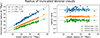 |
Fig. B.1. Left panel: Mean radius inferred from the posterior distribution vs effective radius of the corresponding Voronoi cloud with different truncation thresholds of rVoro > 0 (blue); 0.37 (orange); 0.72 (green). Right panel: Ratio of the radii estimated in the two different ways, after subtracting the y axis offset, which is in the order of a few h−1 Mpc for all cases. The relation is linear for all three cases, and provides information on the threshold to impose in order to achieve a certain depth in the void profile. |
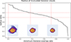 |
Fig. B.2. Radius of the truncated clouds with respect to the statistical radius of the voids, as a function of the Voronoi overlap rate threshold. The small panels illustrate the cloud at different truncation levels: when no threshold is applied, the outskirts are larger than the effective volume represented with the wire-frame sphere; a minimum overlap rate of 0.37 preserves the statistical volume, while larger thresholds yield the very interior of the voids. We illustrate the ∼80% selection, corresponding to rVoro > 0.72, but deeper cuts can be applied if one wishes to probe the most underdense regions. |
Appendix C: Complete catalog
In this section, we expand the discussion presented in the main text to the full catalog. Figure C.1 shows slices of the sky in equatorial coordinates in different redshift bins. In Table C.1 we present the extended version of Table 1, illustrating all the voids in the catalog. The first 3 columns represent the coordinates of the center in the sky, in terms of equatorial coordinates and distance. Column 4 represents the redshift range from the nearest to the farther edge of the void along the line of sight, assuming the effective radius as isotropic size. Columns 5-7 represent summary properties of the posterior distributions for the effective radius and the center position, using the mean and standard deviation. In our cartesian coordinates system the observer is located at [340.5, 340.5, 340.5]h−1 Mpc, with the xy plane corresponding to the equatorial plane, and the  axis pointing to the equatorial north pole. Visual representations of each void in terms of Voronoi clouds can be found in the last columns of the same table presented in the public website: https://voids.cosmictwin.org/VoidGallery. A movie is available online [VoidsGalacticCoord.gif]
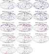 |
Fig. C.1. Different redshift slices representing the sky in Galactic coordinates, with the zero longitude point in the center. The black dots represent the 2M++ galaxies used to infer the posterior realizations of the Local Universe. The crosses represent the void centers within the redshift bin, while the solid circles are the apparent size of their effective radii. The semitransparent circles represent the intersection with voids centered in adjacent redshift bins. We show the neighboring voids only when they intersect the redshift bin entirely, to minimize the visual contamination from galaxies outside of the void. Additionally, the spherical approximation becomes less accurate the farther away from the void center. As a visual confirmation, voids actually occupy the regions with little to no galaxies. The predictive power of the Manticore-Local suite combined with our void finding procedure is shown by the fact that we are able to infer voids behind the Galactic plane, in regions where we do not have direct observations of galaxies. |
Complete void catalog as described in Appendix C.
All Tables
All Figures
|
Fig. 1. Visual representation of our catalog of 100 voids in the local neighborhood within a distance of ≈200h−1 Mpc. The color scale represents the Voronoi overlap rate, i.e., how often a point is contained in a void in different realizations. This quantity is loosely related to the density profile of voids, with high values representing the innermost underdense regions, while lower values are at the edges. The clouds are truncated at the value of 0.37 in order to preserve the statistical volume of all voids. Finally, the wire-frame spheres mark the effective volume of each void. The Cartesian axes are centered on the observer, the xy plane corresponds to the equatorial plane, and the |
| In the text | |
|
Fig. 2. Left panel: Centers of voids with radius 30 < r < 50 h−1 Mpc from all realizations, overlapped on a slice of the 3D space with thickness 60 h−1 Mpc. The dashed blue circle is centered on the observer, and it corresponds to a radius of ≈250 Mpc ≈ 170 h−1 Mpc, encompassing the volume with observed galaxies in 2M++ (where the constraints are more reliable) with interior points marked in red, and the other points plotted in orange. The unconstrained region outside the dashed black square presents a random distribution and can be used to assess the probability of having a cluster of n points by random chance. Central panel: Halo field averaged over all the MCMC realizations. The z thickness is 60 h−1 Mpc and matches the slice in the left panel. Right panel: Visual superposition of the two previous panels. |
| In the text | |
|
Fig. 3. Histogram of the distribution of the void radii for the catalog of high-significance voids (blue) and for the average distribution of individual simulations (orange). The y-axis shows the actual number in each radius bin for the high-significance voids. The orange curve is arbitrarily rescaled to make it comparable. The two histograms illustrate how smaller voids in a single realization of the large-scale structure are more likely to be spurious or less significant, with only a fraction of them contributing to the final catalog. |
| In the text | |
|
Fig. 4. Left panel: Full Voronoi cloud of an example void around its center. The color scale represents the Voronoi overlap rate, ranging from 0 to 1, i.e., how likely a point is to belong to the void throughout different realizations. This value is loosely related to the actual underlying probability distribution, with the yellow regions corresponding to the innermost underdense environment. The wire-frame sphere in the middle represents the effective volume of the void, and the Voronoi cloud extends significantly beyond this region. Right panel: Voronoi cloud truncated to make values of Voronoi overlap rate greater than 0.37, as interpolated from the linear fit of Figure B.1 in Appendix B. The outskirts are removed, and the remaining cloud conserves the mean volume inferred from the Bayesian analysis, while still retaining information on the shape of the void. |
| In the text | |
|
Fig. 5. Representation of void 10, our best candidate to be the well-known Local Void, on a slice of the average halo field with thickness equal to the effective radius Rvoid. The yellow star represents the mean posterior of the center, while the circle is as large as the mean effective volume. The black contours represent the truncated Voronoi cloud, i.e., all the points with rVoro > 0.37, marginalized over the line of sight, obtained by summing the values over the z direction. We normalized this probability distribution to a range between 0 and 1, the contour lines are the 0 and 0.5 levels. The profiles follow perfectly the structure of the underlying field, confirming the quality of the reconstruction. However, the projection does not fully capture the three dimensional information, and heavily depends on the thickness of the density field slab. A representation of different slices on the z-axis can be found at this link: https://voids.cosmictwin.org |
| In the text | |
|
Fig. 6. Sky representation in Galactic coordinates, with the zero longitude point in the center, in two adjacent redshift slices with 0.03 < z < 0.035 and 0.035 < z < 0.04. The black dots represent the 2M++ galaxies used to infer the posterior realizations of the Local Universe. The crosses represent the void centers within the redshift bin, while the solid circles are the apparent size of their effective radii. The semitransparent circles represent the intersection with voids centered in adjacent redshift bins. We show the neighboring voids only when they intersect the redshift bin entirely, to minimize the visual contamination from galaxies outside of the void. Additionally, the spherical approximation becomes less accurate the farther away from the void center. As a visual confirmation, voids actually occupy the regions with little to no galaxies. The predictive power of the Manticore-Local suite combined with our void finding procedure is shown by the fact that we are able to infer voids behind the Galactic plane, in regions where we do not have direct observations of galaxies. The remaining redshift slices are shown in Figure C.1 in Appendix C. A movie is available online [VoidsGalacticCoord.gif]. |
| In the text | |
|
Fig. A.1. Toy model illustrating the continuous binning strategy. The top left panels represents samples of a radius distribution, the top right of the position around the true center. Some nuisance smaller voids are added. The bottom panels represent the result of the technique, with the probability distribution of the radius estimated through a weighted kernel density estimation (KDE). Despite some differences, we find a good match in the mean and standard deviation of the ground truth vs estimate distributions (represented with the error bars on top). A full animation of the procedure can be found here: https://voids.cosmictwin.org/VoidClustering. A movie is available online [moving_bins.gif]. |
| In the text | |
|
Fig. B.1. Left panel: Mean radius inferred from the posterior distribution vs effective radius of the corresponding Voronoi cloud with different truncation thresholds of rVoro > 0 (blue); 0.37 (orange); 0.72 (green). Right panel: Ratio of the radii estimated in the two different ways, after subtracting the y axis offset, which is in the order of a few h−1 Mpc for all cases. The relation is linear for all three cases, and provides information on the threshold to impose in order to achieve a certain depth in the void profile. |
| In the text | |
|
Fig. B.2. Radius of the truncated clouds with respect to the statistical radius of the voids, as a function of the Voronoi overlap rate threshold. The small panels illustrate the cloud at different truncation levels: when no threshold is applied, the outskirts are larger than the effective volume represented with the wire-frame sphere; a minimum overlap rate of 0.37 preserves the statistical volume, while larger thresholds yield the very interior of the voids. We illustrate the ∼80% selection, corresponding to rVoro > 0.72, but deeper cuts can be applied if one wishes to probe the most underdense regions. |
| In the text | |
|
Fig. C.1. Different redshift slices representing the sky in Galactic coordinates, with the zero longitude point in the center. The black dots represent the 2M++ galaxies used to infer the posterior realizations of the Local Universe. The crosses represent the void centers within the redshift bin, while the solid circles are the apparent size of their effective radii. The semitransparent circles represent the intersection with voids centered in adjacent redshift bins. We show the neighboring voids only when they intersect the redshift bin entirely, to minimize the visual contamination from galaxies outside of the void. Additionally, the spherical approximation becomes less accurate the farther away from the void center. As a visual confirmation, voids actually occupy the regions with little to no galaxies. The predictive power of the Manticore-Local suite combined with our void finding procedure is shown by the fact that we are able to infer voids behind the Galactic plane, in regions where we do not have direct observations of galaxies. |
| In the text | |
Current usage metrics show cumulative count of Article Views (full-text article views including HTML views, PDF and ePub downloads, according to the available data) and Abstracts Views on Vision4Press platform.
Data correspond to usage on the plateform after 2015. The current usage metrics is available 48-96 hours after online publication and is updated daily on week days.
Initial download of the metrics may take a while.